Running head: Exposure assessment of L. monocytogenes in goat-cheese 1
Retrospective analysis of a Listeria monocytogenes contamination episode in
2
raw milk goat cheese using quantitative microbial risk assessment tools
3 4
L. Delhalle a*, M. Ellouze b, M. Yde c, A. Clinquart a, G. Daube a and N. Korsak a
5 6
a University of Liège, Faculty of Veterinary Medicine, Department of Food Science,
Sart-7
Tilman, B43bis, 4000 Liege, Belgium 8
b IFIP, French Institute for Pig and Pork Products, Fresh and Processed Meats Department, 7
9
Avenue du Général de Gaulle, 94 704 Maisons Alfort, France. 10
c Scientific Institute of Public Health, Bacteriology section, Rue Juliette Wytsmanstraat 14,
11 1050 Brussels, Belgium. 12 13 *Corresponding author: 14
University of Liège, Faculty of Veterinary Medicine, Department of Food Science, Sart-15
Tilman, B43bis, 4000 Liege, Belgium 16
Tel: 32 4 366 40 40, fax: 32 4 366 40 44 17
Email address: l.delhalle@ulg.ac.be (L. Delhalle) 18
19
Keywords: Exposure assessment; goat-cheese; L. monocytogenes; sensitivity analysis; risk 20
mitigation 21
22 23
Abstract
24In 2005, the Belgian authorities reported a Listeria monocytogenes contamination episode in 25
cheese made from raw goat’s milk. The presence of an asymptomatic shedder goat in the herd 26
caused this contamination. On the basis of data collected at the time of the episode, a 27
retrospective study was performed using an exposure assessment model covering the 28
production chain from the milking of goats up to delivery of cheese to the market. Predictive 29
microbiology models were used to simulate the growth of L. monocytogenes during the 30
cheese process in relation with temperature, pH and water activity. The model showed 31
significant growth of L. monocytogenes during chilling and storage of the milk collected the 32
day before the cheese production (median increase of 2.2 log CFU/ml) and during adjunction 33
of starter and rennet to milk (median increase of 1.2 log CFU/ml). The L. monocytogenes 34
concentration in the fresh unripened cheese was estimated to be 3.8 log CFU/g (median). This 35
result is consistent with the number of L. monocytogenes in the fresh cheese (3.6 log CFU/g) 36
reported during the cheese contamination episode. A variance-based method sensitivity 37
analysis identified the most important factors impacting the cheese contamination, and a 38
scenario analysis then evaluated several options for risk mitigation. Thus, by using 39
Quantitative Microbial Risk Assessment (QMRA) tools, this study provides reliable 40
information to identify and control critical steps in a local production chain of cheese made 41
from raw goat’s milk. 42
The safety of soft cheese made from raw milk is debated with regards to several micro-44
organisms of concern such as Salmonella, enterohemorrhagic E. coli, toxin-producing 45
Staphylococcus aureus and Listeria monocytogenes (9). Cheese made from raw milk may be 46
an important source of human listeriosis (16, 30, 31). 47
In 2005, a Listeria monocytogenes contamination episode in goat cheese made from raw milk 48
was reported by the Belgian Federal Food Agency for the Safety of the Food Chain (FASFC). 49
Using the collected information, we have undertaken a retrospective study based on a 50
quantitative microbial risk assessment (QMRA) method. QMRA is a scientifically based 51
method for modelling the fate of pathogenic micro-organisms along the food chain and for 52
assessing the associated risk of developing adverse effects for the consumer (27). Selected 53
QMRA tools could be used to focus only on the food process and to provide options to reduce 54
the level of contamination of the final product. 55
Field and laboratory collected data were used to implement the exposure assessment model 56
from the milking of the goats up to the storage of end products in the farm. The final output is 57
the L. monocytogenes contamination of goat cheese made from raw milk, due to the presence 58
in the herd of an asymptomatic milk-shedder goat. The model was established in accordance 59
with the Codex Alimentarius Commission guidelines (13). Dynamic predictive microbial 60
models were used to follow the bacterial population during food processing by taking into 61
account the temperature, pH and water activity (38). Sensitivity analysis was performed to 62
identify the most important factors impacting L. monocytogenes concentration in the cheese 63
(40). Finally, valuable options for risk mitigation were proposed and evaluated using scenario 64
analysis. 65
MATERIALS AND METHODS
67
Description of the herd. The herd is composed of 350 goats from the “Alpine” breed. The 68
farm is located in Wallonia (southern part of Belgium). The feed distributed to the goats is 69
mainly composed of hay and grass silage with low moisture and made from herbages stored 70
by the farmer himself. The goats’ milking yield is estimated to average 3.1 litres per goat per 71
day (fat content and average total protein content of 3.1% and 3.4%, respectively). 72
The farmer and the veterinarian have suspected cases of listeriosis among the goats, 73
especially in winters with extremely cold conditions or when molds were observed on hay or 74
silages. The following symptoms were observed in the animals: nervous signs (e.g. ataxia), 75
blindness or reduction of sight ability and spontaneous abortions. No analyses were 76
performed on clinical specimens to confirm the diagnosis. 77
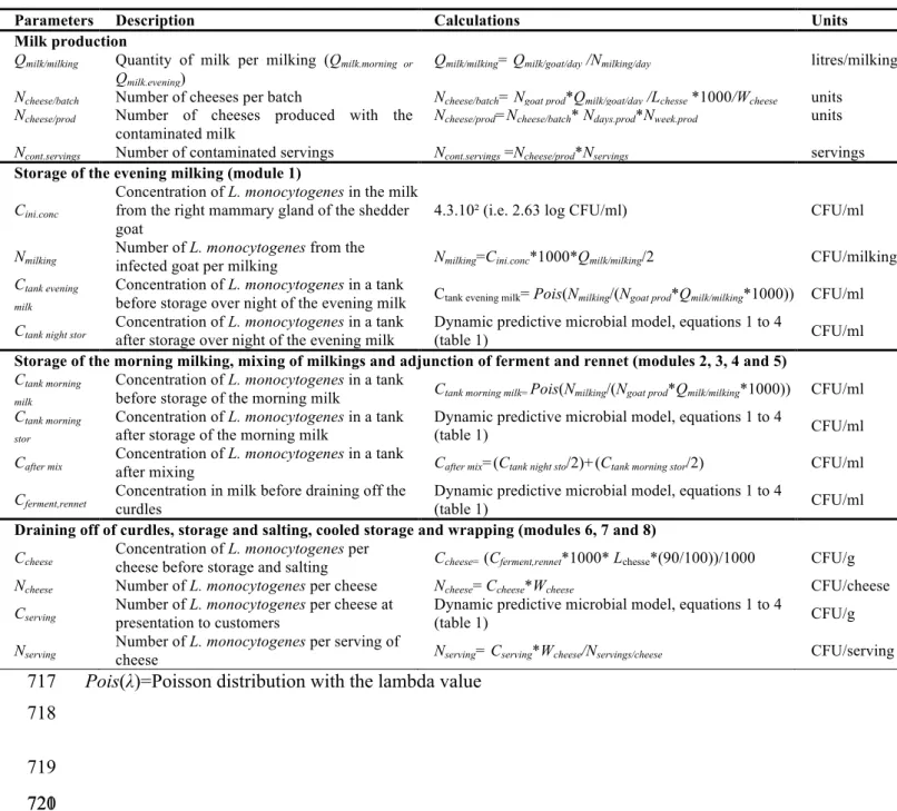
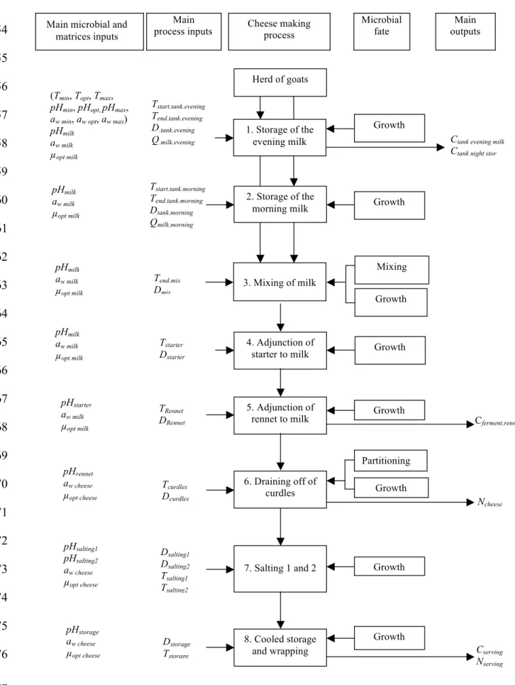
The cheese making process. The cheese production is based on several steps as shown in 78
Figure 1. Tables 1 and 2 describe the inputs and the calculations used in the model. The first 79
step is to refrigerate and cool the evening milk production from 39.5°C to 10°C during 14h. 80
During this step, the growth of L. monocytogenes is possible, and the step was simulated 81
attempting to replicate the temperature evolution, pH (6.63) and water activity (1) of the milk. 82
As a second step, the milk of the morning is collected at 39.5°C, and stored during 1h. 83
L. monocytogenes growth is also possible during this second step. The evening production is 84
then mixed with the morning production and the raw milk mixture is allowed to settle during 85
1h at room temperature in order to achieve an internal temperature of 21-22 °C. A commercial 86
starter culture (PAL Bioprotect D and Pal LC Mix 6, Standa, Caen, France) is added to the 87
raw milk without heating. The starter is received by the processor in the form of a powder that 88
is reconstituted by mixing 200 g in 1 litre of milk to form the “stock solution”. Milk is seeded 89
by adding 20 ml of the “stock solution” to 100 litres of raw milk and is then kept at 22°C for a 90
duration of 2h in order to start the fermentation process. In the fifth step, commercial rennet 91
(présure simple Berthelot®, laboratories Abia, Meursault, France) is added to the fermented 92
milk (15 ml/100 litres raw milk). The mixture is then allowed to settle at 22°C for an 93
additional period of 22h. The next step consists of draining off the water by ladling the fresh 94
cheese (the curds) into plastic molds at 22°C. Molds are turned over three hours later. After 95
0,5h, the cheeses are separated from the molds, placed on metallic racks and stored in a dryer 96
room with an air temperature of between 14.5 and 18°C and relative humidity of 70 to 75%. 97
The seventh step is salting. This operation is repeated twice. Cheeses are first manually turned 98
over and hand-salted on their external surfaces at a temperature of 20°C during 24h. They are 99
replaced back in the dry room, after which they are salted on the other side during 48h at 100
16°C. The final products are cooled during 48h in the chilling room (with a relative humidity 101
of close to 100%) at 1°C until distribution. 102
The main cheese production on this farm is of unripened fresh cheese, but other 103
productions are sometimes performed. For non-fresh cheese, the previous diagram is 104
completed by a ripening step that may last 6 to 7 days, during which cheeses are turned over 105
daily. Some cheeses are dried off in an automatic apportioner or distributor. The drying off 106
may also take place in cellulose bags or in a cheese strainer. The cheeses’ final presentations 107
may also vary. 108
The number of portions of 100g-cheeses produced in a week is estimated to be 5,000 109
cheeses in average, from which 95 % are fresh (not ripened). Around five liters are necessary 110
to produce 1 kg of fresh cheese (due to the loss of whey during the process). 111
Technological analysis performed by the farmer. The farmer uses the Dornic Acidity 112
as a quality indicator during the production process. One Dornic acid degree (°D) is 113
equivalent to 1 mg of lactic acid in 10 ml of milk or 0.1 g/L (23). This test is performed on the 114
milk before fermentation to gain a rough assessment of its hygienic quality and on the curds 115
to monitor the decrease in pH. 116
Microbiological analysis. Once the contamination episode was identified by the FASFC, 117
several microbiological investigations were conducted. An external accredited laboratory 118
performed these analyses. L. monocytogenes was detected on milk and cheese samples using 119
the horizontal method NF EN ISO 11290-1 (3). The method NF EN ISO 11290-2 was used to 120
quantify L. monocytogenes in the samples (4). 121
Technological analysis. To characterize changing factors during the cheese making 122
process, several technological parameters were measured at different stages done at the time 123
of the outbreak by the accredited laboratory. These parameters were: 124
• pH: Laboratory method derived from the ISO 2917:1999 (2), using a Knick 125
765 Laboratory pH meter (Escolab, Kruibeke, Belgium). 126
• Water-activity (aw): method based on the ISO 21807:2005 (5) using a Novasina
127
TH200 water activity meter (Lachen, Switzerland). 128
• Salt content: Laboratory own method adapted the ISO 1841-1:1996 (1). 129
Further characterization of isolates. After identification of the species, the Belgian 130
national reference lab serotyped the isolates ((Institute of Public Health (IPH), Brussels, 131
Belgium) according to a standard protocol using a commercial agglutination test (Denka 132
Seiken, Tokyo, Japan) based on antibodies specifically reacting with somatic (O) and flagellar 133
(H) antigens (46). 134
Susceptibility of the strains to ten antibiotics was determined (Etest, AB BIODISK). 135
Susceptibility to arsenic and cadmium was also performed by the method described in the 136
literature (33). 137
Pulsed-Field Gel Electrophoresis (PFGE) was applied in accordance with the US PulseNet 138
protocol describing PFGE after DNA digestion with the enzymes ApaI and AscI. PFGE 139
enables the cutting of genomic DNA into a number of fragments comprised between 10 and 140
20, that facilitates the computer analysis. The regular change of the current direction in the gel 141
allows the migration of DNA fragments (26). Analysis of banding patterns was performed 142
with an ImageMaster video documentation system (Amersham Pharmacia Biotech) and 143
Fingerprinting II Informatix software (Bio-Rad). 144
QMRA applied to L. monocytogenes in raw goat’s milk cheese – hazard 145
identification. In this study, the hazard is L. monocytogenes and the final output of the 146
exposure assessment model is the level of contamination of raw goat’s milk cheese. 147
L. monocytogenes is ubiquitous and is described as a short rod, catalase-negative, Gram 148
positive micro-organism with a special motility at 25°C (29). In animals this bacterium has 149
been observed since 1926 and has been recognized as a major food borne pathogen since the 150
1980s. It is an intracellular pathogen that can cause a sometimes fatal human disease named 151
“listeriosis”, especially prevalent among high-risk populations, namely the elderly (>60) and 152
immuno-compromised patients. In particular, L. monocytogenes can cause spontaneous 153
abortion in pregnant women as well as meningitis and septicaemia in newborn infants and 154
immuno-compromised people. The case-fatality risk can reach 34% (9). 155
According to the report of the European Food Safety Authority (EFSA), the number of 156
reported cases of confirmed human listeriosis was estimated to be 1,381 in 2008 (21). De 157
Buyser et al. (16) have reviewed the relationship between food borne diseases outbreaks and 158
milk products in France for the period from 1988 to 1997. This study showed that, when the 159
food vehicle was precisely known, milk products accounted for 6% of the outbreaks caused 160
by food borne pathogens. 161
In 1995 “Brie de Meaux” cheese was identified as the source of 36 listeriosis human 162
cases (including 11 deaths), while in 1997 Livarot Pont-L’évêque cheese was implicated in 14 163
cases (16, 30). 164
In Belgium, many cases of listeriosis are not reported in the official statistics since most 165
cases of human listeriosis cause mild to moderate self-limited disease, and the patient does 166
not automatically consult a physician. Moreover, it remains difficult to assess the number of 167
human listeriosis caused specifically by the ingestion of contaminated cheese made from raw 168
goat’s milk. Vanholme et al. (47) reported that the number of cases of listeriosis officially 169
reported in Belgium in 2005 was 40, but different food sources were involved including beef, 170
pork, dairy products, fish and ready-to-eat products (RTE). It was therefore not possible to 171
estimate the number of listeriosis claerly attributable to cheese made from raw goat’s milk. 172
However, a serotyping comparison was possible. In 2005 serotypes 1/2a caused 55 % of cases 173
of listeriosis reported in Belgium and serotype 4b caused 42.5% (47). 174
QMRA applied to L. monocytogenes in raw goat’s milk cheese – exposure assessment. 175
Fresh unripened cheese was chosen for the exposure assessment model because it is the most 176
sold product. Furthermore, data for this product are available to support a retrospective 177
investigation. The principles of the Modular Process Risk Model (MPRM) methodology were 178
used to break down the food production chain into modules (36) and to follow the 179
bacteriological concentration of the pathogen throughout the process, including the eight 180
modules presented in Figure 1: (1) storage of the evening milk, (2) storage of the morning 181
milk, (3) mixing of the morning and evening milk, (4) adjunction of the starter to the milk, (5) 182
adjunction of rennet to the milk, (6) draining off of curds, (7) salting at ambient temperature 183
and (8) cooled storage. Each module generates an output that is used as an input for the next 184
module. The simulated events are identified for each module: growth, mixing and/or 185
partitioning. Input values are classified as process inputs, microbiological or food 186
characteristics. Table 1 describes parameters as fixed values or probability distributions 187
reflecting the natural variability. 188
Growth was simulated using primary and secondary predictive microbiology models. 189
A three phase linear model without lag was used to simulate the growth of 190
L. monocytogenes as a function of time (11) as shown in Equation 1. 191
193
Equation 1
195
where i is one of the eight modules of the process with i = 1 to 8 196
k is the recorded parameter index in the stage i with k = 1,...,n 197
Δtk is the time interval with Δtk = 1 hour
198
Ntk is the bacterial population at time tk (CFU.ml-1 or CFU.g-1)
199
Nmax is the maximal bacterial population (CFU.ml-1 or CFU.g-1)
200
The effects of temperature, pH and water activity on the maximum growth rate µmax of
201
L. monocytogenes were modelled by a multiplicative function with interaction (Equation 2) 202
derived from the cardinal model (Equation 3 and 4) (8, 14): 203 ) , , ( ) ( ) ( ) ( ( ) 1 ( ) 1 ( ) ( ) ( ) ( ) 2 ) ( maxik
µ
optCM Tik CM pHik CM awikξ
Tik pHik awikµ
= Equation 2 204 205 Equation 3 206 207 208 209 210 and € θ=0,5. Equation 4 211 212where µmax i(k) is the bacterial growth rate following the environmental factors at time tk
213
Ti(k) is the recorded temperature at time tk (°C)
214
pHi(k) is the recorded pH at time tk
215
awi(k) is the recorded water activity at time tk
216 € CMn(X ) = 0, (X − Xmax)(X − Xmin) n (Xopt− Xmin) n−1(X
opt− Xmin)(X − Xopt) − (Xopt− Xmax) (n −1)X
(
opt+ Xmin− nX)
[
]
0, # $ % % & % % € X ≥ Xmax € Xmin< X < Xmax ! " ! # $ ≥ < < − ≤ = 1 , 0 1 ), 1 ( 2 , 1 ) , , ( ( ψ ψ θ ψ θ ψ ϕ ξ T pH aw € X ≤ Xmin € ln( Ntk) = ln( Ntk −1) +µmaxi(k )Δtk = ln( Nmax) , if € Nt k< Nmax , if € Ntk≥ Nmax∑
⋅∏
− = ≠ i j i j i x X )) ( 1 ( 2 ) (ω
ω
ψ
with 3 min ) ( ! ! " # $ $ % & − − = X X X X X opt opt ω ,Xmin, Xopt and Xmax, are the minimal, optimal and maximal temperature, pH and water
217
activity of growth for L. monocytogenes. 218
Table 2 gives the calculation details to assess the final number of L. monocytogenes in a 219
typical serving of fresh goat cheese. 220
The starting point of the model is the initial concentration of L. monocytogenes in the 221
milk from the right part of the mammary gland of the contaminated goat (4.3.102 CFU/ml or 222
2.63 log CFU/ml ; source: FASFC). This concentration is used in the first module to calculate 223
the L. monocytogenes number per milking and to deduce the concentration of 224
L. monocytogenes in the tank before the overnight storage of the evening milking. It is 225
assumed that this concentration is a Poisson distribution and that the milk temperature 226
decreases linearly overnight between the beginning and the end of the cooling. There is no 227
heat exchanger plate in the food process. The temperature of the evening milk decreases 228
slowly in the tank overnight. Predictive microbiology models simulate the growth of 229
L. monocytogenes during this storage period. 230
The second module is dedicated to the storage of the morning milking, where the 231
L. monocytogenes concentration in the tank before the storage of the morning milk is assessed 232
and implemented in predictive microbiology models to simulate the pathogen evolution in the 233
tank after the morning storage. The initial temperature of this second module corresponds to 234
the temperature at the end of the milking, 39.5°C, while the final temperature obtained after 235
one hour storage is sampled among a Pert distribution, with a most likely final temperature of 236
22°C and minimum and maximum final temperatures of 20 and 24°C, respectively. It is 237
explained by the mixing of the evening and the morning milk in the same tank at the end of 238
the storage of the morning milk. 239
In the third module, the concentration of the pathogen in the tank after mixing is 240
deduced from the concentrations of L. monocytogenes in the tank before and after storage to 241
be implemented in modules 4 and 5 representing the steps of starter and rennet adjunction to 242
milk. Using predictive microbiology models (equations 1 to 4), the L. monocytogenes 243
concentration in milk before draining off the curdles is calculated. It is assumed that the 244
distribution of the pathogen is heterogeneous during the curdling of milk. Following Bemrah 245
et al. (9), the Listeria cells concentrates at a level of 90 % in the curds and 10 % in the whey. 246
The start and end temperatures of this step are sampled among a Pert distribution, with a most 247
likely value of 22°C and minimum and maximum values of 20 and 24°C, respectively. The 248
pH is considered to decrease linearly between the start and the end of the fermentation 249
process according to equation 5. 250 i pH t pH=−0.1005 + Equation 5 251
This linear relation is based on the evolution of pH and Dornic acidity with time in the 252
fermented milk (data not shown). A correlation was made between the values of Dornic 253
acidity measured by the farmer and the pH measurements in the laboratory. 254
The concentration in milk before draining off the curdles is used in module 6 to assess 255
the amount of pathogen per cheese before storage and salting. Finally, in modules 7 and 8, 256
predictive microbiology models are used to characterize the number of L. monocytogenes per 257
serving of cheese, taking into account the effects of temperature, pH and aw as shown in
258
Figure 1. 259
Technological parameters measured in the milk and at different stages of ripening of 260
the final product (2 measurements per sample) are used according to Table 1 and 2. 261
The model was developed using @Risk 4.5.5 (Palisade, Ithaca, N.Y.), an add-in for 262
Microsoft Excel. Input values of each module were implemented as estimated distributions of 263
probability, to describe the natural variability associated with input factors. We used 50,000 264
iterations with the latin hypercube sampling (LHS) method to obtain stochastic estimates of 265
the output variables (32). Finally, the estimated median concentration of L. monocytogenes in 266
a serving of cheese was compared with the concentration measured in the fresh cheese by the 267
FASFC. 268
QMRA applied to L. monocytogenes in raw goat’s milk cheese – sensitivity analysis. In order 269
to identify the subset of the most important factors of the exposure assessment model, a global 270
sensitivity analysis (SA) was performed using the Saltelli method (40). This is a numerical 271
based procedure for computing first order indices, Si, and total effect indices, Sti, for all the
272
factors i (i=1,…,k) of the studied model. Each first order index Si provides an estimate of the
273
relative importance of the factor Xi taken singularly, while the total effect index Sti reflects the
274
cooperative effects of the factor Xi and its non linear interactions with the other factors (40,
275
41). The method is fully described in the literature (40-44). Its implementation for microbial 276
growth models is provided in Ellouze et al. (20), and recently this method was applied to a 277
QMRA of L. monocytogenes in deli meats (12). 278
To calculate these indices, a characterization of the range of variation of the several 279
factors of the model is necessary. These factors are presented in Table 3 and are composed of 280
two categories of factors. The first category includes factors related to the milk production 281
such as the number of goats and the quantity of milk per milking. The second category 282
includes factors representing the characteristics of the pathogen such as its cardinal values, its 283
optimum growth rates in milk and cheese, etc. 284
A total set of 35 input factors was thus identified for the exposure assessment model. 285
Their ranges of variation were obtained directly from experimental data provided by the 286
farmer (minimum and maximum observed values) or from the 1st and 99th percentiles of the 287
distributions characterizing their variability. 288
Once the ranges of variation of the different input factors were characterized, their indices 289
were computed according to the following procedure. Two matrices A and B of N lines 290
corresponding to the N simulation runs (N=5.104) and k columns corresponding to the k 291
studied factors (k=35) were generated using the LHS method as a space filing design. The 292
matrices A and B were filled with respect to the range of variation of each factor (Table 3) 293
and the model was run on each row of the two matrices to provide the response vectors YA and
294
YB. Then, k matrices Ci, i=1,…,k, were generated, containing all the columns of matrix B
295
except the ith column which was replaced by the ith column of matrix A, and the global model 296
was run again to provide the vectors YCi. Finally, the first order indices, Si, and total effect
297
indices, Sti, were calculated according to the following formula (40):
298 299 300 301 302 303 with
∑
∑
= = N u u B u A N u u A Y Y N g Y N f 1 ) ( ) ( 0 1 ) ( 0 1 1 304The bootstrap method (18) was used to assess the confidence intervals of these indices 305
through reliable estimates without additional computational effort (6). Values obtained for the 306
response vectors were sampled with replacement for 104 bootstrap replicates, and, for each
307
replicate, the indices Si and Sti were calculated, leading to a bootstrap estimate of the
308
distribution of the sensitivity indices. The 95% confidence intervals of the indices were thus 309
defined using the 5th and 95th percentiles and were used to identify the most important factors
310
as those for which the total effect indices were significantly different from 0. 311
QMRA applied to L. monocytogenes in raw goat’s milk cheese – Scenario analysis. 312
The effect of some variables in the exposure assessment model was assessed using simulation 313
scenarios to provide valuable information on possible ways of reducing the concentration of 314 2 0 1 ) ( ) ( 0 1 ) ( ) ( 1 1 f Y Y N g Y Y N S N u u A u A N u u i C u A i − − =
∑
∑
= = 2 0 1 ) ( ) ( 2 0 1 ) ( ) ( 1 1 1 f Y Y N f Y Y N St N u u A u A N u u i C u B i − − − =∑
∑
= = Equation 6pathogens in a final serving (17, 48). This assessment was achieved by selecting various 315
combinations of input variables. 316
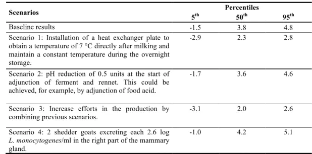
This procedure is commonly known as a “what if scenario” (49). In the present study, a 317
first run of the model without modifications was performed to provide the baseline results of 318
the selected outputs. Three scenarios were tested in order to look for ways of reducing the 319
risk, and one worst-case scenario was tested to assess the magnitude of the risk increase in 320
such a case: 321
• Scenario 1: Install a heat exchanger plate to obtain a temperature of 7 °C directly after 322
milking and maintain a constant temperature during the overnight storage. 323
• Scenario 2: Reduce pH by 0.5 units at the start of adjunction of ferment and rennet. This 324
could be achieved, for example, by adjunction of a common food acid such as lactic acid 325
or glucono delta lactone. 326
• Scenario 3: Increase efforts during production by combining Scenarios 1 and 2. 327
• Scenario 4: Two shedder goats in the herd each excreting the same amount of 328
L. monocytogenes as the goat on the farm studied. 329
Decontamination treatments, such as pasteurization, are not considered to respect the 330
initial characteristics of the product. The results are displayed as the concentration of 331
L. monocytogenes in a cheese serving. 332
RESULTS
333
Alert investigations. Table 4 summarizes the information in relation to the anamnesis of 334
the case. 335
The serotyping results of the first external laboratory showed that the strain isolated from the 336
cheese belongs to serotype 1/2a with a characteristic β-hemolysis. Three days later another 337
external laboratory analyzed the pools of milk collected from the goats. One positive pool 338
(milk collected from twenty goats) was detected, and from the sources of that milk one clearly 339
positive goat was identified in the herd. 340
The goat was transferred to the Faculty of Veterinary medicine. The results of milk 341
samples were as follows: 342
• 2.6 log L. monocytogenes /ml in the milk collected from the right part of the mammary 343
gland 344
• absence of L. monocytogenes in 25 g of the milk collected from the left part of the 345
mammary gland 346
Enumerations were also made on the cheeses with the following results: 347
• concentration of L. monocytogenes in fresh not ripened goat cheese: 3.6 log CFU/g 348
• concentration of L. monocytogenes in ripened goat cheese: 3.8 log CFU/g 349
• concentration of L. monocytogenes in ripened goat cheese coated with charcoal: 3.7 350
log CFU/g 351
352
The L. monocytogenes isolates collected from the milk and cheese were sensitive to the 10 353
investigated antibiotics and were sensitive to arsenic and cadmium. 354
The pulsotyping results showed that isolates from the milk of the isolated goat and from 355
the contaminated cheese belonged to the same pulsovar A (data not shown). In 2005, the 356
Belgian Listeria reference laboratory received 40 strains of L. monocytogenes of human 357
clinical origin: 16 strains were of serovar 1/2a, of which 7 strains were arsenic and cadmium 358
sensitive. However, pulsotyping excluded genetic matching for these 7 strains with the cheese 359
and milk isolates from the goat farm (data not shown). This means that no cases of human 360
listeriosis could be traced back to the consumption of the contaminated goat cheese. 361
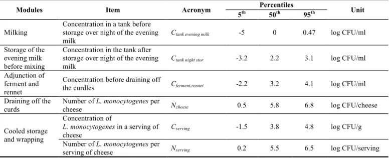
QMRA model – baseline results. Table 5 gives the base line results of the exposure 362
assessment and the risk characterization modules. Since these models were built to take into 363
account the natural variability associated with the different input factors, the results are 364
expressed as distributions. The median estimates (50th percentile) associated with the 5th and
365
95th percentiles presented in Table 5 give a good assessment of the results. L. monocytogenes
366
concentrations results are converted to a logarithmic scale (base 10). 367
The modular exposure assessment model shows a significant growth of L. monocytogenes 368
during chilling and storage of the milk collected the day before the cheese production (an 369
increase of 2.2 log CFU/ml for the median). Figure 2a gives the pathogen evolution at this 370
step with dynamic temperature conditions. During the storage of the evening milking 371
overnight, the milk is slowly chilled from 39.5°C to 10°C. The growth rate of 372
L. monocytogenes is directly related to the temperature, which explains the observed brake of 373
microbial growth during the chilling process. 374
A less important increase (1.2 log CFU/ml for the median) was obtained after the starter 375
and rennet adjunction to milk. This result is explained by the pH drop in the milk due to the 376
fermentation activity, which gradually decreased the pH down to 4.41. Figure 2b shows the 377
evolution of L. monocytogenes after the adjunction of ferment and rennet. At the end of the 378
fermentation, the pH value was close to the minimum pH for L. monocytogenes growth 379
(pHmin=4.19), which can explain the limited growth of the pathogen after the fermentation.
380
The estimated median L. monocytogenes concentration in a serving of cheese (Table 5) 381
was equal to 3.8 log CFU/g. This estimate was in compliance with the concentration of 382
L. monocytogenes reported in the fresh cheese by the FASFC during the contamination 383
episode, which was equal to 3.6 log CFU/g. The model gives satisfactory results by 384
comparison with the data provide by the FASC. 385
Sensitivity analysis. The global sensitivity analysis results are depicted in Table 6, which 386
presents the first order and total effect indices of each factor with their confidence bootstrap 387
intervals. 388
Total effect indices and first order indices are especially powerful when performing SA in 389
cases of non additive and non linear models (6) such as the exposure assessment part of the 390
model used in this study. In fact, as can be deduced from Table 6, the sum of the non negative 391
first order indices (Si), which account for the individual contribution of each factor into the
392
variance of the output, is less than 1, which means that the variance of the output cannot be 393
explained solely by the sum of the individual effects of each factor, but is also attributed to 394
the effects of interactions. 395
This is also confirmed by the relatively substantial difference observed between the Sti
396
and the Si for all the important factors, which indicates the significant role of interactions.
397
Ranking the 35 factors of the model according to their total effect indices identified the most 398
important factors. Total effect indices were chosen as ranking criteria because they indicate 399
the effect of each studied factor and its interactions with the other factors. They were 400
therefore preferred to the first order indices, which only reflect the relative importance of the 401
factor taken singularly. 402
The confidence intervals associated with the total effect indices were examined, and the 403
factors with confidence intervals significantly different from 0 were identified as the most 404
important factors. Four factors were thus selected: the duration of the first salting step 405
(Dsalting1), the minimum pH for L. monocytogenes growth pHmin, the optimal growth rate of
406
L. monocytogenes in milk (µopt_milk) and the initial L. monocytogenes concentration (N0).
407
Scenario analysis. The results of the scenario analysis are displayed in Table 7. The 408
outputs are the amount of L. monocytogenes per cheese serving. The results obtained for the 409
first scenario show a reduction of 1.5 log CFU/g compared with the baseline results and could 410
be a good alternative for risk mitigation. The results obtained for the second scenario prove 411
that a reduction of 0.5 pH units could only reduce by 0.2 log CFU/g the median concentration 412
compared with the baseline results. The results obtained for the third scenario, which 413
combines Scenarios 1 and 2, show a reduction of 1.8 log CFU/g of the median concentration 414
compared with the baseline results. The last scenario shows a significant increase of 0.4 log 415
L. monocytogenes/g in a cheese serving compared with the baseline results. 416
DISCUSSION
417
Few QMRA concerning cheese contaminated with L. monocytogenes have been published 418
(9, 22). This is probably due to the difficulty of obtaining valuable data to develop a complete 419
QMRA of the cheese production chain. In fact, a frequently heard criticism of QMRA is that 420
it is extremely data hungry (27), and its final results depend heavily on the quality of the input 421
data, particularly when variability and uncertainty are taken into account. 422
In an attempt to simulate the entire production chain of cheese made from raw goat‘s 423
milk, an exposure assessment that takes into account different sources of natural variability 424
was developed in this study. The results showed a significant growth of L. monocytogenes 425
during the cheese manufacturing process, especially after the evening milk storage (median 426
increase of 2.2 log CFU/ml) and during the steps of starter and rennet adjunction to milk 427
(median increase of 1.2 log CFU/ml). 428
However, it is thought that the acidification process experienced during cheese making is 429
not favourable to pathogen growth. In fact, Schvartzman et al. (45) have shown that there was 430
no growth of L. monocytogenes 4b isolated from cow faeces during the process of cheese 431
making from raw cow’s milk, but growth was observed on the same process when pasteurized 432
milk was used, which is probably due to the absence of a competitive flora. Some studies 433
have already reported the importance of the presence and/or the level of the competitive flora 434
on the growth/no growth of L. monocytogenes in several foods (25, 34). The model developed 435
in this study did not specifically include the effect of the competitive flora, but the simulated 436
median result for the L. monocytogenes concentration in the fresh cheese was equal to 3.8 log 437
CFU/g which was consistent with the concentration of L. monocytogenes (3.6 log CFU/g) 438
detected by the FASFC in the contaminated fresh cheese. This result does not constitute a 439
validation, it means only that the model seems to have a good behaviour with the collected 440
data. 441
Due to the lack of data, this exposure assessment model like any other may suffer 442
descriptive errors that represent incorrect or insufficient information (24). In fact, the lack of 443
data sometimes made it necessary to build in several assumptions. First, the storage 444
temperature of the evening milking was considered to decrease linearly during the night. 445
Some authors have attempted to model the temperature evolution during the cheese making 446
process (28), but as the linear decrease in temperature gave satisfactory simulated 447
temperatures compared to the observed temperatures, this assumption was adopted to avoid 448
over-parameterization of the exposure assessment model. Second, the excretion of 449
L. monocytogenes by the contaminated shedder goat was considered to be the same for each 450
production day. Third, L. monocytogenes distribution was supposed to be heterogeneous 451
during the curdling of milk with a level of 90 % in the curds and 10 % in the whey. This last 452
assumption was based on the study of Bemrah et al. (9). 453
In spite of these limitations, this study attempts to simulate the contamination flow of raw 454
goat cheese produced on a local dairy farm and to relate the final concentration of 455
L. monocytogenes in cheese with observed epidemiological and microbiological data made in 456
a contamination alert episode in 2005. 457
This study also suggests risk mitigation scenarios to reduce the concentration of 458
L. monocytogenes at the end of the cheese process. The first scenario considered a faster 459
chilling of the milk from the initial temperature of 39.5 °C down to 7 °C. At this temperature, 460
the growth rate of L. monocytogenes is considerably reduced during the storage of the milk 461
over night, resulting in a reduction of 1.5 log CFU/g in the final concentration of the pathogen 462
in the cheese. The second scenario evaluated a pH reduction of 0.5 units at the start of the 463
adjunction of ferment and rennet. This intervention could be simply achieved by lactic acid 464
adjunction, for example, and could reduce the median growth of L. monocytogenes by 0.2 log 465
CFU/g. The third scenario, which is a combination of the previous two, showed a reduction of 466
1.8 log CFU/g of the median L. monocytogenes concentration compared with the model 467
baseline results. The last scenario, involving two shedder goats in the herd, showed a 468
significant increase of 0.4 log L. monocytogenes concentration in a serving cheese compared 469
with the base line results. 470
The results of the sensitivity analysis gave complementary information and identified four 471
factors significant for their impact on the concentration of L. monocytogenes in cheese. 472
Among the four significant factors, pHmin and µopt_milk are characteristics of the pathogen for
473
which it is therefore impossible to control. However, the sensitivity analysis also uncovered 474
the potential to act on technological parameters, such as the salting time to reduce the number 475
of contaminated cheeses. It is also feasible to perform effective actions to reduce the initial 476
contamination level N0. Efficient and frequent monitoring of the pathogen in the food chain
477
could significantly reduce its concentration in the end product and could be easily achieved by 478
means of a more stringent sampling plan for the raw milk and cheese. 479
In the future it would be interesting to identify sources of L. monocytogenes 480
contamination. A few studies have explored sources of contamination on farms. Danielsson-481
Tham et al. (15) studied an outbreak of gastro-intestinal listeriosis affecting 120 humans in 482
Sweden after consumption of raw-milk cheese produced in a summer farm composed of dairy 483
cattle and goats. The authors traced back the origin of contamination in the cheese by 484
investigating the different sources in the summer farm and in the cheese production facilities. 485
The most likely hypothesis, although not strictly confirmed, was the presence of a goat in the 486
herd with a subclinical mastitis which led to the contamination of equipment in the cheese 487
production facilities, specifically a wooden bench and the home-made brine. Nightingale et al. 488
(37) explain that the patterns of contamination on farms are not very clear: is the feed the 489
main source of infection in animals and hence in the milk products or is the animal itself? 490
Grazing seems not to be the predominant route of infection, but poorly made silages (e.g. corn 491
silages with a high end-pH value) may lead to an amplification of the levels of Listeria 492
species in animals. Comparing the prevalence of Listeria monocytogenes on case farms 493
(farms with a history of animal listeriosis) and on control farms (farms with no reports of 494
animal listeriosis) they observed that for small ruminants the prevalence was higher on case– 495
farms. Yet, for cattle the prevalence was statistically equivalent between case and control 496
farms. 497
Faecal contamination of the animals may explain the greater prevalence of listeriosis in 498
small ruminants on case farms. If it is the cause, then faecal contamination may also increase 499
the likelihood of Listeria monocytogenes contamination of raw milk. The fact that patterns of 500
contamination appear quite different between the cattle and the goat populations led 501
Danielsson-Tham et al. (15) to conclude that some ribotypes may be able to persist in the 502
environment and others not. Wiedmann et al. (51) also concluded that multiple ribotypes may 503
exist on a farm at the same time, colonizing differently depending on environmental factors, 504
because the researchers observed in only one case a relationship between the strains isolated 505
in clinical samples of animals and strains isolated from silages. In our study, we assume that 506
the contamination of raw milk occurred mainly through the milk, even though Listeria 507
monocytogenes could have been recovered from the faecal matter of the asymptomatic 508
shedder goat. 509
Meyer-Broseta et al. (35), using different sampling strategies, noticed that Listeria 510
monocytogenes occurs at a very low level in the tank. When the bulk tanker in the milk 511
processing industry was contaminated (collecting different deliveries from cattle farms), the 512
average prevalence for positive farms was 7.7% with contamination levels for 513
L. monocytogenes below 3 CFU/ml and a median of between 5.10-2 and 1.10-1 CFU/ml.
514
Several authors have noticed that it is important to have a final pH-value in the silages that is 515
lower than 5 in order to decrease the risk of listeriosis in ruminants (50, 51). In our case, the 516
farmer observed a significant decrease of listeriosis cases in the goats after he had adapted his 517
machine for producing hay and low-moisture grass-silages. He began cutting the grass higher, 518
which may have reduced the contamination of the hay and silages by dirt and dust from the 519
soil. This decrease in contamination may explain the decrease in observed cases of listeriosis 520
in the goats. The farmer also observed that the remaining cases of listeriosis were more 521
frequent during the winter season, which is consistent with findings in the scientific literature 522
(10). 523
In conclusion, this retrospective study aims to simulate the fate of L. monocytogenes 524
throughout a raw goat’s milk cheese making process from milking to delivery to the market, 525
using quantitative microbial risk assessment methodology. The results were satisfactory when 526
compared with the epidemiological and microbiological observations of the alert 527
investigations. The most important factors of the L. monocytogenes contamination were 528
identified, and risk mitigation scenarios were evaluated to identify the most efficient 529
strategies to reduce the risk of listeriosis in respect of the food characteristics. 530
Due to the lack of data for some parameters, the exposure assessment was based on 531
several assumptions. Although continued work is needed to better evaluate risks to 532
consumers, this study clearly demonstrated that QMRA tools and predictive modelling can be 533
useful to increase food safety and should be gradually implemented in the coming years. 534
References 535
536
1. Anonymous. 1996. ISO 1841-1 Viande et produits à base de viande - 537
Détermination de la teneur en chlorures. Partie 1 : méthode de Volhard. p. 1-4. In ISO 538
(International Organization for Standardisation), Genève (in French). 539
2. Anonymous. 1999. ISO 2917:1999(F) Viande et produits à base de viande - 540
mesurage du pH - méthode de référence p. 1-6. In ISO (International Organization for 541
Satndardization), Genève (In French). 542
3. Anonymous. 2004. NF EN ISO 11290-1 Méthode horizontale pour la recherche et 543
le dénombrement de Listeria monocytogenes. Partie 1 : Méthode de recherche - 544
Amendement 1 : modification des milieux d'isolement, de la recherche de l'hémolyse et 545
introduction de données de fidélité. Horizontal method for the detection and 546
enumeration of Listeria monocytogenes. Part 1 : Detection method - amendment 1: 547
modification of the isolation media, of the haemolysis test and inclusion of precision 548
data. p. 1-14. In CEN (European Committee for Standardisation), Bruxelles (in 549
French). 550
4. Anonymous. 2004. NF EN ISO 11290-2 Méthode horizontale pour la recherche et 551
le dénombrement de Listeria monocytogenes. Partie 2 : Méthode de dénombrement. 552
Amendement 1 : Modification du milieu d'isolement. Horizontal method for the 553
detection and enumeration of Listeria monocytogenes. Part 2: Enumeration method. 554
Amendment 1: modification of the enumeration medium. p. 1-4. In CEN (European 555
Committee for Standardisation), Bruxelles (in French). 556
5. Anonymous. 2005. NF ISO 21807 Microbiologie des aliments - Détermination de 557
l'activité de l'eau. p. 1-8. In ISO (International Organization for Standardization) 558
Genève (in French). 559
6. Archer, G. E. B., A. Saltelli, and I. M. Sobol. 1997. Sensitivity measures, 560
ANOVA-like techniques and the use of bootstrap. J. Statist. Comput. Simul. 58:99–120. 561
7. Augustin, J. C. 1999. Modélisation de la dynamique de croissance des populations 562
de Listeria monocytogenes dans les aliments. p. 157. In, vol. PHD. Université de Lyon, 563
Lyon. 564
8. Augustin, J. C., V. Zuliani, M. Cornu, and L. Guillier. 2005. Growth rate and 565
growth probability of Listeria monocytogenes in dairy, meat and seafood products in 566
suboptimal conditions. J. Appl. Microbiol. 99:1019-42. 567
9. Bemrah, N., M. Sanaa, M. H. Cassin, M. W. Griffiths, and O. Cerf. 1998. 568
Quantitative risk assessment of human listeriosis from consumption of soft cheese made 569
from raw milk. Prev Vet Med. 37:129-45. 570
10. Brugère-Picoux, J. 2008. Ovine listeriosis. Small Ruminant Res. 76:12-20. 571
11. Buchanan, R. L., R. C. Whiting, and W. C. Damert. 1997. When is simple good 572
enough: a comparison of the Gompertz, Baranyi, and three-phase linear models for 573
fitting bacterial growth curves. Food Microbiol. 14:313-326. 574
12. Busschaert, P., A. H. Geeraerd, M. Uyttendaele, and J. F. Van Impe. 2011. 575
Sensitivity Analysis of a Two-Dimensional Quantitative Microbiological Risk 576
Assessment: Keeping Variability and Uncertainty Separated. Risk Anal. 31:1295-1307. 577
13. Codex Alimentarius Commission. 1999. Principles and guidelines for the conduct 578
of microbiological risk assessment. Codex Alimentarius Commission, Roma. 579
14. Couvert, O., A. Pinon, H. Bergis, F. Bourdichon, F. Carlin, M. Cornu, C. Denis, 580
N. Gnanou Besse, L. Guillier, E. Jamet, E. Mettler, V. Stahl, D. Thuault, V. Zuliani, and 581
J.-C. Augustin. 2010. Validation of a stochastic modelling approach for Listeria 582
monocytogenes growth in refrigerated foods. Int. J. Food Microbiol. 144:236-242. 583
15. Danielsson-Tham, M. L., E. Eriksson, S. Helmersson, M. Leffler, L. Ludtke, M. 584
Steen, S. Sorgjerd, and W. Tham. 2004. Causes behind a human cheese-borne outbreak 585
of gastrointestinal listeriosis. Foodborne Pathog. Dis. 1:153-159. 586
16. De Buyser, M. L., B. Dufour, M. Maire, and V. Lafarge. 2001. Implication of milk 587
and milk products in food-borne diseases in France and in different industrialised 588
countries. Int. J. Food Microbiol. 67:1-17. 589
17. Delhalle, L., C. Saegerman, W. Messens, F. Farnir, N. Korsak, Y. Van der Stede, 590
and G. Daube. 2009. Assessing interventions by quantitative risk assessments tools to 591
reduce the risk of human salmonellosis from fresh minced pork meat in Belgium. J. 592
Food Prot. 72:2252-2263.
18. Efron, B., and R. J. Tibshirani. 1993. An introduction to the bootstrap. Chapman 594
& Hall, New York. 595
19. Ellouze, M., and J. C. Augustin. 2010. Applicability of biological time 596
temperature integrators as quality and safety indicators for meat products. Int. J. Food 597
Microbiol. 138:119-129.
598
20. Ellouze, M., J. P. Gauchi, and J. C. Augustin. 2011. Use of global sensitivity 599
analysis in quantitative microbial risk assessment: Application to the evaluation of a 600
biological time temperature integrator as a quality and safety indicator for cold smoked 601
salmon. Food Microbiol. 28:755-769. 602
21. European Food Safety Authority. 2010. The Community Summary Report on 603
Trends and Sources of Zoonoses, Zoonotic Agents, Antimicrobial Resistance and 604
Foodborne Outbreaks in the European Union in 2008. p. 496. In, EFSA Journal, vol. 8. 605
European Food Safety Authority, Parma. 606
22. Farber, J. M., W. H. Ross, and J. Harwig. 1996. Health risk assessment of Listeria 607
monocytogenes in Canada. Int. J. Food Microbiol. 30:145-56.
608
23. Fondation de Technologie Laitière du Québec. 2002. Science et technologie du 609
lait. Transformation du lait. Presses internationales polytechnique, Montreal. 610
24. Garrido, V., I. García-Jalón, A. I. Vitas, and M. Sanaa. 2010. Listeriosis risk 611
assessment: Simulation modelling and "what if" scenarios applied to consumption of 612
ready-to-eat products in a Spanish population. Food Control. 21:231-239. 613
25. Gnanou Besse, N., N. Audinet, L. Barre, A. Cauquil, M. Cornu, and P. Colin. 614
2006. Effect of the inoculum size on Listeria monocytogenes growth in structured media. 615
Int. J. Food Microbiol. 110:43-51.
616
26. Graves, L. M., and B. Swaminathan. 2001. PulseNet standardized protocol for 617
subtyping Listeria monocytogenes by macrorestriction and pulsed-field gel 618
electrophoresis. Int. J. Food Microbiol. 65:55-62. 619
27. Havelaar, A. H., E. G. Evers, and M. J. Nauta. 2008. Challenges of quantitative 620
microbial risk assessment at EU level. Trends Food Sc. Technol. 19:S26-S33. 621
28. Iezzi, R., S. Francolino, and G. Mucchetti. 2011. Natural convective cooling of 622
cheese: Predictive model and validation of heat exchange simulation. J. Food Eng. 623
106:88-94. 624
29. International Commission on. Microbiological Specifications for Foods. 1996. 625
Microorganism in foods. Characteristics of Microbial pathogens. Blackie Academic & 626
Professional, London. 627
30. Jacquet, C., C. Saint-Cloment, F. Brouille, B. Catimel, and J. Rocourt. 1998. La 628
listeriose humaine en France en 1997, données du Centre National de Référence des 629
Listeria. Bulletin épidémiologique hebdomadaire. 33.
630
31. Jacquet, C., F. Brouille, C. Saint-Cloment, B. Catimel, and J. Rocourt. 2000. La 631
listériose humaine en France en 1998 -- données du Centre national de référence des 632
Listeria. Journal de Pédiatrie et de Puériculture. 13:120-122.
32. McKay, M. D., R. J. Beckman, and W. J. Conover. 1979. A comparison of three 634
methods for selecting values of input variables in the analysis of output from a computer 635
code. Technometrics. 21:239-245. 636
33. McLauchlin, J. 1997. The identification of Listeria species. Int. J. Food Microbiol. 637
38:77-81. 638
34. Mellefont, L. A., T. A. McMeekin, and T. Ross. 2008. Effect of relative inoculum 639
concentration on Listeria monocytogenes growth in co-culture. Int. J. Food Microbiol. 640
121:157-168. 641
35. Meyer-Broseta, S., A. Diot, S. Bastian, J. Riviere, and O. Cerf. 2003. Estimation 642
of low bacterial concentration: Listeria monocytogenes in raw milk. Int. J. Food 643
Microbiol. 80:1-15.
644
36. Nauta, M. J., . 2001. A modular process risk model structure for quantitative 645
microbiological risk assessment and its application in an exposure assessment of Bacillus 646
cereus in a REPFED. p. 100. In National Institute of Public Health and the
647
Environment, Bilthoven. 648
37. Nightingale, K. K., Y. H. Schukken, C. R. Nightingale, E. D. Fortes, A. J. Ho, Z. 649
Her, Y. T. Grohn, P. L. McDonough, and M. Wiedmann. 2004. Ecology and 650
transmission of Listeria monocytogenes infecting ruminants and in the farm 651
environment. Appl. Environ. Microbiol. 70:4458-4467. 652
38. Pouillot, R., and M. B. Lubran. 2011. Predictive microbiology models vs. 653
modeling microbial growth within Listeria monocytogenes risk assessment: What 654
parameters matter and why. Food Microbiol. 28:720-726. 655
39. Rosenow, E. M., and E. H. Marth. 1987. Growth of Listeria monocytogenes in 656
skim, whole and chocolate milk and whipping cream during incubation at 4, 8, 13, 21 657
and 35°C. J. Food Prot. 50:452-459. 658
40. Saltelli, A. 2002. Making best use of model evaluations to compute sensitivity 659
indices. Comput. Phys. Commun. 145:280-297. 660
41. Saltelli, A. 2002. Sensitivity Analysis for Importance Assessment. Risk Anal. 661
22:579-590. 662
42. Saltelli, A., M. Ratto, T. Andres, F. Campolongo, J. Cariboni, D. Gatelli, M. 663
Saisana, and S. Tarantola. 2008. Global Sensitivity Analysis :The primer. Chichester, 664
West Sussex, England. 665
43. Saltelli, A., S. Tarantola, and F. Campolongo. 2000. Sensitivity Analysis as an 666
Ingredient of Modeling. Stat. Sci. 15. 667
44. Saltelli, A., S. Tarantola, F. Campolongo, and R. Marco. 2007. Sensitivity 668
Analysis in practice : A guide to assessing scientific models. Chichester, West Sussex, 669
England. 670
45. Schvartzman, M. S., A. Maffre, F. Tenenhaus-Aziza, M. Sanaa, F. Butler, and K. 671
Jordan. 2011. Modelling the fate of Listeria monocytogenes during manufacture and 672
ripening of smeared cheese made with pasteurised or raw milk. Int. J. Food Microbiol. 673
145:531-538. 674
46. Seeliger, H. P. R., and K. Höhne. 1979. Chapter II Serotyping of Listeria 675
monocytogenes and Related Species. p. 31-49. In T. Bergan, and J.R. Norris (ed.),
676
Methods in Microbiology, vol. Volume 13. Academic Press. 677
47. Vanholme, L., H. Imberechts, G. Ducoffre, and K. Dierick. 2009. Report of 678
zoonotic agents in Belgium in 2007. p. 164. In The Veterinary and Agrochemical 679
Research centre, Brussels. 680
48. Vose, D. 2000. Risk analysis A quantitative guide. John Wiley & Sons Inc, 681
Chichester. 682
49. Vose, D. 2005. ModelAssist Advanced for @Risk. In V. Consulting (ed.) Risk 683
Thinking Ltd, Gent. 684
50. Wiedmann, M., J. Czajka, N. Bsat, M. Bodis, M. C. Smith, T. J. Divers, and C. A. 685
Batt. 1994. Diagnosis and epidemiological association of Listeria monocytogenes strains 686
in two outbreaks of listerial encephalitis in small ruminants. . J. Clin. Microbiol. 32:991-687
996. 688
51. Wiedmann, M., J. L. Bruce, R. Knorr, M. Bodis, E. M. Cole, C. I. McDowell, P. 689
L. McDonough, and C. A. Batt. 1996. Ribotype diversity of Listeria monocytogenes 690
strains associated with outbreaks of listeriosis in ruminants. J. Clin. Microbiol. 34:1086-691 90. 692 693 694
List of tables
695696
Table 1: Characterization of the model inputs ... 33 697
Table 2: Calculation details to assess the contamination of a serving of cheese ... 35 698
Table 3: Identification of input factors for the sensitivity analysis and their respective 699
ranges of variation ... 36 700
* measured values ... 36 701
Table 4: Anamnesis elements in relation to the carrier animal ... 37 702
Table 5: Baseline results of the exposure assessment and the risk characterization 703
modules 39 704
Table 6: Estimates of the first order (Si) and total effect (Sti) indices of the sensitivity
705
analysis and their bootstrap confidence intervals (p5 and p95) ... 40 706
Table 7: Results of the scenarios analysis (Concentration of L. monocytogenes in a cheese 707
(log CFU/g)) 41 708
33 le 1: Cha ra cte ri za tion of the m ode l i nput s Ch ee se m ak in g p ro ce ss Pa ra m et er De sc rip tio n Va lu es / D ist rib u tio n s Un its 0. C har ac te riz at ion of the m ilk pr oduc tion N goat Nu m be r o f go ats 350 goa ts N goat pr od Nu m be r o f g oa ts fo r t he c he es e p ro du cti on P (1 60 ;1 70 ;1 80 ) goa ts N cont am inat ed.goat Nu m be r o f c on ta m in ate d g oa ts fo r t he c he es e p ro du cti on 1 goa ts Q mi lk /g oa t/d ay Qu an tit y o f m ilk p er g oa t pe r da y P (2 .5 ;3 ;3 .5 ) litr es /d ay N mi lk in g/d ay Nu m be r o f m ilk in gs pe r da y 2 tim es /d ay L chesse Nu m be rs o f l itr es p er 1 Kg o f c he es e P (4 ;5 ;5 .5 ) litr es W cheese We ig ht of c he es e P (9 5;1 00 ;1 05 ) g N days. pr od Nu m be r o f d ay s f or c he es e p ro du cti on p er we ek 5 da ys N we ek .p ro d Nu m be r o f we ek s o f pr oduc tion w ith the c ont am ina te d m ilk 19 we ek s N servi ngs/ cheese Nu m be r o f s er vin gs pe r c he es e 2 se rv in gs 1. St or age of the e ve ni ng m ilk T st art .tank. eveni ng In iti al te m pe ra tu re o f m ilk c oll ec te d i n t he e ve nin g 39. 5 °C T end.t ank.eveni ng Fi na l te m pe ra tu re o f m ilk c oll ec te d i n t he e ve nin g P (9 ;1 0;1 2) °C D ta nk .e ve nin g Du ra tio n o f t he e ve nin g m ilk st or ag e o ve rn ig ht P (1 3;1 4;1 5) h 2. St or age of the m or ni ng m ilk T st art .tank. m orni ng In iti al te m pe ra tu re o f m ilk c oll ec te d i n t he m orn in g 39. 5 °C T end.t ank.m orn in g Fi na l te m pe ra tu re o f m ilk c oll ec te d i n t he m or nin g P (2 0;2 2;2 4) °C D ta nk .m or nin g Du ra tio n o f t he m or nin g m ilk st or ag e b ef or e m ix in g 1 h 3. M ix ing T end.m ix Mi lk te m pe ra tu re a fte r m ix in g P (2 0;2 2;2 4) °C D mi x Du ra tio n o f t he st ep m ix in g o f t he m or nin g an d ev en in g m ilk 1 h 4. A dj unc tion of st ar te r T st art er Mi lk te m pe ra tu re a t th e s te p a dju nc tio n o f s ta rte r P (2 0;2 2;2 4) °C D st art er Du ra tio n o f t he st ep a dju nc tio n o f s ta rte r 2 h pH st art er pH a t the e nd of the st ep adj unc tion of st ar te r 6. 3 pH uni ts 5. Ad ju nc tio n o f r en ne t T rennet Mi lk te m pe ra tu re a t th e a dju nc tio n o f r en net P (2 0;2 2;2 4) °C D rennet Du ra tio n o f t he st ep a dju nc tio n o f r en net 22 h pH rennet pH a t the e nd of the st ep adj unc tion of ren net 4.41 pH uni ts 6. D rai ni ng of f c ur dl es T curdl es Te m pe ra tur e a t the st ep dr aini ng of f c ur dl es P (2 0;2 2;2 4) °C D curdl es Du ra tio n o f t he st ep d ra in in g o ff cu rd le s 0. 5 h 7. Sal tings 1 and 2 T sal ting1 Te m pe ra tu re a t th e s te p S alt in g 1 P (1 9;2 0;2 1) °C D sal ting1 Du ra tio n o f t he st ep S alt in g 1 24 h pH sal ting1 Fi na l p H o bta in ed a fte r t he st ep Sa lti ng 1 4. 28 pH uni ts T sal ting2 Te m pe ra tu re a t th e s te p S alt in g 2 P (1 4;1 6;1 8) °C D sal ting2 Du ra tio n o f t he st ep S alt in g 2 48 h pH sal ting2 Fi na l p H o bta in ed a fte r t he st ep Sa lti ng 2 4. 42 pH uni ts 8. C ool ed stor age T st orage Te m pe ra tu re o f t he c oo le d s to ra ge P (0 ;1 ;2 ) °C D st orage Du ra tio n o f t he c oo le d s to ra ge 48 h