Reassessing the Gender Wage Gap in Madagascar: Does Labour Force Attachment Really Matter?

(1)

DIAL • 4, rue d’Enghien • 75010 Paris • Téléphone (33) 01 53 24 14 50 • Fax (33) 01 53 24 14 51 E-mail : dial@dial.prd.fr • Site : www.dial.prd.fr

D

OCUMENT DE

T

RAVAIL

DT/2005-06

Reassessing the Gender Wage Gap:

Does Labour Force Attachment

Really Matter? Evidence from

Matched Labour Force and

Biographical Surveys in Madagascar

Christophe J. NORDMAN

François ROUBAUD

(2)

REASSESSING THE GENDER WAGE GAP: DOES LABOUR FORCE

ATTACHMENT REALLY MATTER? EVIDENCE FROM MATCHED LABOUR

FORCE AND BIOGRAPHICAL SURVEYS IN MADAGASCAR

1

Christophe J. Nordman IRD-Paris, DIAL nordman@dial.prd.fr François Roubaud IRD-Paris, DIAL roubaud@dial.prd.fr

Document de travail DIAL Juin 2005

ABSTRACT

Differences in labour force attachment across gender are important to explain the extent of the gender earnings gap. However, measures of women's professional experience are particularly prone to errors given discontinuity in labour market participation. For instance, the classical Mincerian approach uses potential experience as a proxy for actual experience due to lack of appropriate data. Such biases in the estimates cannot be ignored since the returns to human capital are used in the standard decomposition techniques to measure the extent of gender-based wage discrimination. Matching two original surveys conducted in Madagascar in 1998 - a labour force survey and a biographical survey enabled us to combine the original information gathered from each of them, particularly the earnings from current employment and the entire professional trajectories. Our results lead to an upward reappraisal of returns to experience, as potential experience always exceeds actual experience, for both males and females. In addition, controlling for further qualitative aspects of labour force attachment, we obtain a significant increase in the portion of the gender gap explained by observable characteristics.

Key words: Gender earnings gap, decompositions, discrimination, returns to human capital, sectoral participation, sample selectivity, biographical survey data, Madagascar

JEL Code: J24, J31, O12.

RESUME

Les différences constatées dans la participation au travail des hommes et des femmes peuvent en partie expliquer les disparités de revenus. Cependant, l’expérience professionnelle des femmes est particulièrement sujette aux erreurs de mesures du fait des interruptions répétées qui jalonnent leur parcours professionnel. Faute de données appropriées, la grande majorité des études sur ce thème doit se contenter d’approcher l’expérience effective dans l’emploi par l’expérience potentielle. Ces erreurs de mesure sont d’autant plus gênantes que les rendements du capital humain sont ensuite mobilisés par les techniques standard de décomposition pour apprécier l’ampleur des discriminations salariales suivant le genre. L’appariement de deux enquêtes réalisées à Madagascar en 1998 – une enquête emploi et une enquête biographique, nous permet de combiner les informations des deux sources, notamment les revenus du travail de la première et l’ensemble de la trajectoire professionnelles de la seconde. Nos résultats conduisent à une réévaluation à la hausse des rendements de l’expérience, aussi bien pour les hommes que pour les femmes. De plus, la part de l’écart de revenus suivant le genre expliquée par les caractéristiques observables des individus augmente significativement.

Mots clés : Ecarts de revenus selon le genre, décompositions, discrimination, rendements du capital humain, participation sectorielle, effets de sélection, enquête biographique, Madagascar

1

We gratefully acknowledge valuable comments from participants in a seminar at DIAL in Paris, in the Minnesota International Economic Development Conference in Minneapolis, in the Journées de l’AFSE in Clermont-Ferrand and in the Annual Conference of the European Society for Population Economics in Paris. Special thanks go to Ragui Assaad, Denis Cogneau, Philippe de Vreyer and François-Charles Wolff for helpful remarks. Usual disclaimers apply.

(3)

BIBLIOGRAPHY ... 45

List of tables

Table 1 : Sample distribution by age group and sex... 10

Table 2 : Labour market dynamics 1995-1998 ... 16

Table 3 : Participation and sectoral job allocation by gender ... 18

Table 4 : Differences in education and labour force attachment for paid work participants... 18

Table 5 : Differences in earnings and human capital across gender and generation ... 19

Table A0 Probit Estimates of Males and Females' Employment Participation ... 30

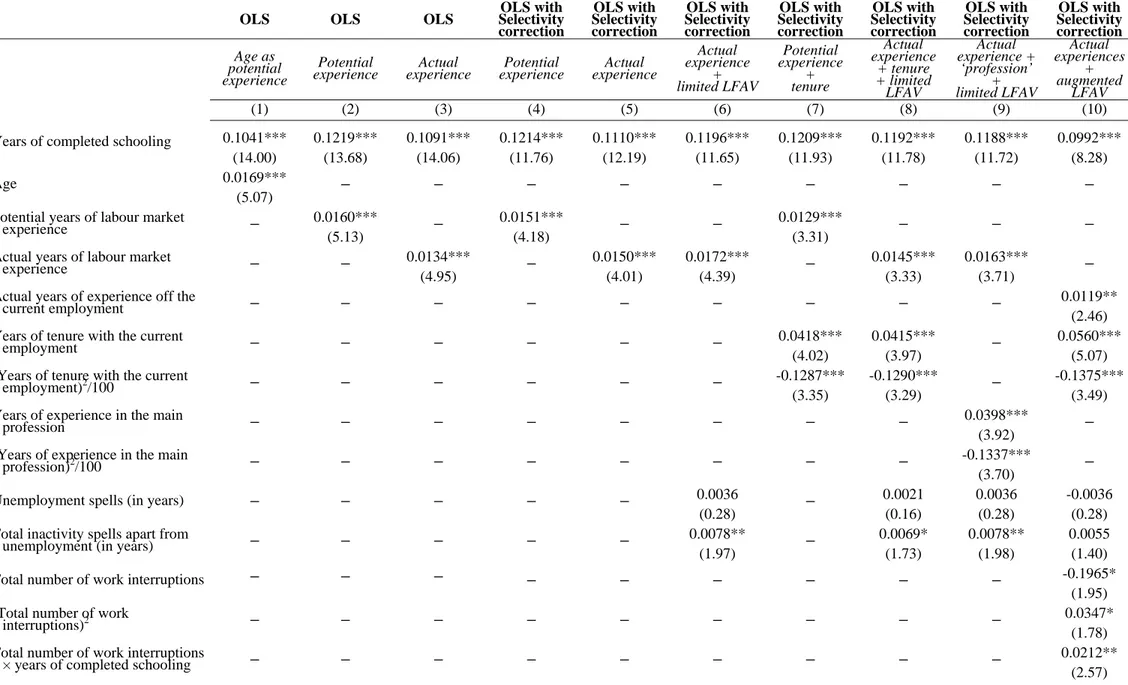
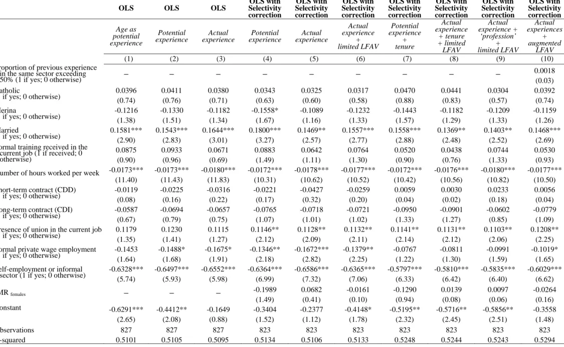
Table A1 Earnings Functions for Males ... 31

Table A2 Earnings Functions for Females ... 33

Table A3 Maximum Likelihood Estimates of Multinomial Logit Sectoral Choice Models ... 35

Table A4 Selectivity Corrected Log Earnings Functions Across Sectors for Males ... 37

(4)

Table A6 Overview of Gender Earnings Decompositions Using Alternative Decomposition Techniques

and Non-Selectivity Corrected Earnings Models ... 41 Table A7 The Oaxaca and Neumark Decompositions Using Selectivity Corrected Earnings Models ... 42 Table A8 The Oaxaca and Neumark Decompositions by Sector Using Selectivity Corrected Earnings

Models ... 43 Table A9 Full Decomposition of Gender Earnings Gap Accounting for Selectivity ... 44

List of figures

Figure 1 : Evolution of GDP and private consumption per capita 1960-1998 ... 16 Figure 2 : Evolution of the job structure by cohort and gender ... 17 Figure 3 : Log hourly earnings of men (1) and women (2) by percentile... 19

(5)

1. INTRODUCTION

Returns to human capital have always been considered dominant explanations for labour compensation. Accordingly, they have been incorporated in individual wage equations by using regressors describing schooling and the worker’s labour market experience2_{. This is particularly} important for developing countries where the returns to education are expected to be higher3_. However, before the 1980s, it was impossible to measure human capital accumulated on the job exactly. Mincer (1974) had indeed already admitted that the representation of post-school investments was the weak point of the theoretical architecture of his model. For the model to be improved, professional investments had to be better specified4_{. He was unable to do this himself, because the data} available at that time did not allow better specifications of post-school investment in human capital. As rightly underlined by Willis (1986, p.543), “the [Mincerian] earnings function represents a pragmatic method of incorporating some of the major implications of the optimal human capital models into a simple econometric framework which can be applied to the limited information available in Census-type data”5. The recommended estimate consisted in using the time spent in certain circumstances, i.e. in the firm or the workplace. Since measures of actual experience were not available when the major empirical developments of the original theory emerged, estimates were established using potential experience, calculated as age minus years of schooling minus age on entering school (generally 6). Refinements were proposed later, as new surveys became available providing more detailed information about the time that individuals had actually devoted to their principal employment. Hence, Mincer and Jovanovic (1981) introduced the workers' tenure in firms to take into account the return to specific training received. The time elapsed in the labour market is assumed to reflect the accumulation of general human capital. The remuneration of experience and tenure therefore represents the return to human capital accumulated on the job. The longitudinal data available today distinguishes more accurately between these two measures and enriches the information used in empirical studies. It is therefore not only possible to calculate more or less exactly the time that an individual has dedicated to work, but also to isolate the experience acquired in various industries and/or jobs. Nowadays, studies using this type of measure are frequent in developed countries, too frequent indeed to be detailed here6_.

These issues are of a great importance in assessing the extent of gender inequalities in urban labour markets. In industrialised countries, many attempts have been made to estimate the extent to which the average gender wage gap is due to differences in human capital attributes such as schooling and work experience, versus differences between genders in wages paid for given attributes. From the literature on this issue, less than half of the gap can be explained by factors such as differences in years of schooling and experience and tenure (Albrecht, Björklund and Vroman, 2003). However, it has been shown that missing or imprecise data on these human capital factors can result in serious biases in the calculation of the discrimination component resulting from Mincerian wage equations.

In fact, measures of women's professional experience are particularly prone to errors given discontinuity in labour market participation. Often age or the Mincer measure of experience and their squared values are still used as a proxy for the acquisition of general human capital or for work experience. Potential experience may be a good approximation of true experience for men with high labour force attachment, but is a poor proxy for less attached individuals, especially for women or minority groups as they have a greater likelihood of interrupting their professional activities (Antecol and Bedard, 2004). Proxy measures tend to overstate women's actual work experience by not accounting for interruptions related to parenting (that is, complete withdrawals from the labour market) or, for instance, for any restrictions on the number of hours worked per week. Furthermore, empirical studies have revealed that experience before an interruption has a lower return than

2 _{Mincer (1993); Card (1999).} 3

Sahn and Alderman (1988), Hoddinott (1996), Behrman (1999).

4_{“[…] the most important and urgent task is to refine the specification of the post-school investment category […] to include details}

(variables) on a number of forms of investment in human capital” (Mincer, 1974, p. 143).

5 _{It is interesting to note that in most LDCs, information on earnings is not available in Census-type data.}

(6)

experience after an interruption (Dougherty, 2003) and that women who interrupt their careers generally receive less wage growth prior to the interruption (Mincer and Polachek, 1974; Sandell and Shapiro, 1980; Mincer and Ofek, 1982). Hence, the coefficient of experience in the wage equation, but also the coefficient of education, may be systematically biased, notably for women7_{. Such biases in the} estimates cannot be ignored since the returns to human capital are used in the standard decomposition techniques for gender wage gaps, and therefore to measure the extent of gender-based wage discrimination (Blinder, 1973; Oaxaca, 1973). Authors have in fact argued that these measurement errors can amplify the impact attributed to pure discrimination (the unexplained part of the wage decomposition), to the detriment of the component relating to observed differences in individual characteristics between men and women (Stanley and Jarell, 1998; Weichselbaumer and Winter-Ebmer, 2003).

In developing countries, especially the poorest ones, the above-mentioned problems are even greater than in developed countries, particularly due to the shortage of available information. At the same time, gender inequality is likely to be greater, markets do not function efficiently and the States lack the resources for introducing corrective policies. Under the PRSP initiative that concerns over sixty of the world's poorest countries, policies designed to counter gender discrimination are among the solutions most often recommended to combat poverty (Cling, Razafindrakoto and Roubaud, 2003). Goal 3 of the Millennium Development Goals (MDG) is aimed at reducing gender inequalities.

In this article, we will cast new light on these issues by using a series of first hand surveys of the labour market carried out in 1998 in the capital of Madagascar, Antananarivo, under the supervision of one of the authors. The approach consists in matching a labour force survey and a biographical survey, in a view to obtaining detailed information on complete professional and family trajectories for a representative sample of the population. The estimated earnings functions and the resulting wage differential decomposition enable us to match the income from current employment, taken from the first survey, with the individuals' actual experience (length and type of jobs occupied, periods of inactivity, unemployment, etc.) over their entire life span, taken from the second. As far as we know, this is the first such attempt at a detailed study of this sort in Africa, which was inaccessible until now due to the lack of appropriate data.

The paper is divided as follows. Section 2 briefly surveys the key contributions to literature on gender wage gap issues, mainly in sub-Saharan Africa. Section 3 presents the two datasets used in this paper, while section 4 discusses the main econometric methods for assessing the gender gap: earning functions and gender wage decompositions. The background of the Madagascan labour market and some descriptive statistics are considered in section 5. In section 6 we turn to the econometric results, obtained with alternative measures of human capital and experience. Finally, in section 7, we draw together the main findings and present our conclusions.

2. ASSESSING THE GENDER WAGE GAP: A REVIEW OF THE LITERATURE ON AFRICA

In the economics literature on developing countries, a few attempts have been made to estimate the extent to which the average gender wage gap is due to differences in human capital attributes such as schooling and work experience, versus differences between genders in wages paid for given attributes. These issues are of great importance in assessing the extent of gender inequalities in urban labour markets.

2.1. Why may returns to labour market experience differ across gender?

First, men and women differ considerably in the amount of time they work and in the continuity of their work experience, especially in Africa. Women are more likely to combine periods of paid work with periods of labour force withdrawal for family-related reasons. This affects job tenure, a factor

7 _{Indeed, it can be shown that underestimating the return to experience can lead in turn to underestimating the return to education if}

(7)

that influences wages. Second, human capital skills may depreciate during long periods of labour force withdrawal. Women returning to the same employer after an interruption in employment may be less likely to be promoted. Or, females not returning to the same employer may have to accept lower wages than they received prior to their withdrawal. Third, some studies in industrialised countries demonstrate that women who interrupt their careers generally receive less wage growth prior to the interruption (Mincer and Polachek, 1974; Sandell and Shapiro, 1980; Mincer and Ofek, 1982). This may be explained by the fact that women expecting several withdrawals from the labour force may postpone training, or may decide to accept low-paid jobs in industries or occupations that are easy to enter and exit. Fourth, the timing of labour force withdrawals may affect wages. Job-related skills are usually acquired at the start of careers – which generally coincides with decisions regarding children. A significant portion of real lifetime earnings growth has been found to occur during the first years after graduation (Murphy and Welch, 1990). If so, the timing of labour force withdrawals may have important long-term implications for future earnings patterns. As a result, there is no reason why the pattern of the marginal returns to labour market experience should be identical in males and females' careers. Moreover, describing these patterns by using the concavity of a declining quadratic function alone – for both sexes – is an excessive or even sometimes false assumption8.

2.2. Gender wage gap: some results for Africa

Appleton, Hoddinott and Krishnan (1999) noticed that there is very little literature on the gender wage gap in Africa. In fact, from a recent meta-analysis of the literature on gender wage gap decomposition, Weichselbaumer and Winter-Ebmer (2003) evaluate that, out of all the empirical studies on the topic since the 1960s, only 3% stem from African data9_.

From the existing literature, there is however a wide consensus on the presence of important inequalities between men and women, both for salaried and self-employed workers. For instance, in Guinea, Glick and Sahn (1997) find that differences in characteristics account for 45% of the male-female gap in earnings from self-employment and 25% of the differences in earnings from public-sector employment while, in the private public-sector, women actually earn more than men.

Armitage and Sabot (1991) also found that such gender inequality exists in the public sector of Tanzania but observed no gender discrimination in Kenya's labour market. The latter result is true both for the public and private sectors of the Kenyan economy. Similarly, Glewwe (1990) found no wage discrimination against women in Ghana. On the contrary, females seem better off than males in the public sector. More recently, Siphambe and Thokweng-Bakwena (2001), using data from the 1995-1996 Labour Force Survey in Botswana, show that in the public sector most of the wage gap is due to differences in characteristics between men and women and not to discrimination on the basis of rewards to those characteristics. On the other hand, in the private sector, most of the wage gap is due to discrimination. Likewise, in Uganda and Côte d'Ivoire, Appleton et al. (1999) find evidence that the public sector practises less wage discrimination than the private sector. However, from their study on Côte d'Ivoire, Ethiopia and Uganda, they finally conclude that there is no common cross-country pattern in the relative magnitudes of the gender wage gaps in the public and private sectors10_.

Other studies have pointed out the role of occupational choices in mediating the gender wage gap. Using survey data from manufacturing firms in Morocco and Tunisia, Nordman (2002a, 2002b, 2004) shows that, ceteris paribus, Tunisian (Moroccan) females earn on average 17% (13%) less than males. But after taking account of firm heterogeneities (by matching data on workers and firms), Nordman (2004) highlights that this gender wage differential, commonly attributed to pure discrimination and/or unobserved individual/firm heterogeneities with standard regression techniques, can be further reduced to 13% and 11% if the omitted information can be controlled for. Furthermore, analyses

8 _{Indeed, Murphy and Welch (1990) noticed that the quadratic curve underestimates the marginal return to tenure at low and very high}

values of tenure. They found that a quartic earnings function might be more appropriate and is preferable in many cases.

9 _{See, notably, Glewwe (1990) for Ghana; Cohen and House (1993) for Sudan; Milne and Neitzert (1994) and Agesa (1999) for Kenya;}

Glick and Sahn (1997) for Guinea; Armitage and Sabot (1991) for Kenya and Tanzania; Appleton, Hoddinott and Krishnan (1999) for Uganda, Côte d'Ivoire and Ethiopia; Isemonger and Roberts (1999) for South Africa; Siphambe and Thokweng-Bakwena (2001) for Botswana and Nordman (2004) for Morocco and Tunisia.

10_{In Uganda, the authors find that the wage gaps in the public and private sector are comparable. In Ethiopia, there is a much wider gap in}

(8)

including job characteristics, such as working conditions, show that workers' job preferences with regard to their educational attainments might be an important factor in explaining wage discrimination in Morocco and Tunisia11_.

Consequently, results from these case studies in Africa suggest the importance of sectoral choices, but also of workers' job status, for analysing differences of wage determination between the sexes.

In Madagascar, the only study we are aware of is that of Nicita and Razzaz (2003). Using household-level data drawn from the Enquête Prioritaire Auprès des Ménages (EPM) carried out by the Institut National de la Statistique (INSTAT) in 1999, the authors investigate the gender wage gap in relation to an analysis of the growing potential of a particular economic sector, the textile industry. From their earnings differential decomposition (Oaxaca, 1973), they show that both the endowments and the unexplained part of the wage difference favour male workers, although the latter dominates the former12_{. Second, education and potential experience (measured by age) are similarly important in} determining the wage differential. Third, level of education and being resident in urban Antananarivo slightly reduce the unexplained part of the wage differential. However, no general conclusion on Madagascar can be drawn from their analysis as it only concerns one particular manufacturing sector. Another limitation of their study is that, as a result of lack of information, they proxy labour market experience by age and include very few regressors in their wage equations by sexes13. As Weichselbaumer and Winter-Ebmer (2003) have shown, this may have serious consequences on the extent to which gender wage discrimination is appreciated (upward biased) because the unexplained gender wage gap can be attributed in this case to the specification error in the original wage regression (i.e. unaccounted characteristics remain correlated with the unexplained component of the gender wage differential).

Humphrey (1987) explains earnings inequalities between men and women (in Brazilian industry) by several factors, including professional segregation. Other studies focus on the role of job structure. Looking at the heterogeneity of the labour market (public, private and informal sectors), various authors demonstrate that earnings gaps result from the sector to which individuals belong (Khandker, 1992; Glick and Sahn, 1997); in this way, women's low incomes can be explained by their concentration in the informal sector. However, the results vary from one country to another. In Guinea, men's income is higher than women's in the informal and public sectors. Men's higher incomes in the informal sector are apparently due to discrimination against women in access to resources (credit) and to training.In the monetized sectors, control for the effect of education reveals a gender bias, revealed in the structure of the jobs occupied by men and women (Glick and Sahn, 1997). Generally speaking, labour market segmentation highlights earnings inequalities that can be explained by differences in human capital endowments and professional segregation. This professional segregation may reflect discriminatory practices (sexist recruitment methods, stereotypes and prejudice against women, etc.) based on what Bourdieu (1998) calls “male domination”, which prevents women from having access to certain well-paid segments or professions.

11_{Indeed, in Morocco and Tunisia, detailed observation of workers in their workplace (Nordman, 2004) revealed that women were often}

employed for performing tasks that were completely disconnected from their skills and qualifications. For instance, the author highlights that it is not uncommon to find women with higher education degrees assigned to unskilled blue-collar jobs.

12_{In 1999, the gross unadjusted wage differential is about 51% in favour of males. The results of the decomposition attribute about 14% to}

differences in endowments. The unexplained part accounts for about 59% of the wage differential, while the remaining 27% is due to selectivity.

13

The determinants introduced in the wage specifications are: level of education, age and a regional dummy for the urban district of Antananarivo. They also control for potential selectivity effects by adding the Inverse Mill's Ratio stemming from a first-step Probit estimation where the probability of being employed by sex is explained by the same regressors as mentioned above plus the individual's number of children, civil status and status of household head. In their wage specification across sexes, the R2 _{amount to 0.37 and 0.084}

(9)

3. THE DATA: MATCHING LABOUR FORCE AND BIOGRAPHICAL SURVEYS

The data used here has been obtained by matching two original surveys conducted in Madagascar in 1998 by the National Institute of Statistics (INSTAT) as part of the MADIO project (Roubaud, 2000):

• the first, a labour force survey, was designed to collect detailed information on employment, unemployment, income and working conditions in the Madagascan capital;

• the second, a biographical survey, followed the trajectories of a representative sample of Tananarivians in three different fields: migratory and residential trajectory, family and marital trajectory and schooling and professional trajectory.

The joint use of these two surveys offers three key advantages for our study. First, this type of survey, whether on labour force or on individual trajectories, is extremely rare in the African context. Second, the data is of a far higher standard than that usually collected in household surveys in Africa. Finally, the fact that the sample used in the biographical survey was a sub-sample of the labour force survey means that the two surveys can be matched on an individual level, thereby enabling us to combine the original information gathered for each of them, particularly the earnings from current employment in the labour force survey and the entire social and professional trajectories in the biographical survey (individual's household characteristics, employment, unemployment, inactivity spells).

3.1. The labour force survey (1-2-3 Survey, Phase 1, 1998)

The labour force survey used in this study corresponds to the first phase of the 1-2-3 Survey, on employment, the informal sector and consumption, carried out in a number of developing countries, in Africa and in Latin America (Razafindrakoto and Roubaud, 2003; Cling et al., 2005). This system of household surveys was introduced for the first time in Madagascar in 1995. The National Institute of Statistics has repeated the operation every year since then. The sample, drawn from a stratified two-stage area-based survey plan, is representative of all ordinary households in the capital of Madagascar. In each household, all individuals of 10 and over, i.e. all the people of working age according to the official nomenclature, were questioned about their labour market participation. The definitions (activity, unemployment, etc.) follow the international standards recommended by the ILO in this respect (Hussmann, Mehran and Verma, 1990). In 1998, for instance, of the 3,002 households questioned, we counted 10,081 people of working age, of whom 5,822 individuals were active wage earners, 361 unemployed and 3,998 inactive. For all those in work, we have a comprehensive set of data on the job characteristics: type of job (profession, job occupied, number of hours worked, income, benefits, type of contract, years of tenure), some characteristics of the firms concerned (institutional sector, including informal sector, branch, size of firm, type of premises, trade union presence, etc.). In addition, we also have detailed data on the individuals' socio-demographic characteristics (gender, age, level of education, ethnic group, religion, migratory status, marital status, etc)14_.

Given that the earnings variable plays a central role in our study, it is important to give a few explanations about how it is measured in the survey. Special attention is given to capturing income derived from work. All occupied wage-earners (i.e. all individuals who worked for at least one hour during the week preceding the interview), are asked about the monthly earnings relating to their main job, for the month preceding the survey. Those who are unable or unwilling to answer the direct question on the amount of their income are encouraged to answer a second, less intrusive, question where they no longer declare a precise sum, but an income bracket, expressed in multiples of the current minimum wage. In the 1998 survey, out of a total of 5,298 active wage-earners, 3,445 declared their actual income and 1,853 declared their income bracket; only 13 individuals refused to provide information on their income, which is in itself an indicator of the quality of the survey. Several alternative methods are then employed to attribute an income to those who only declared an income bracket15_{. The survey also provides an estimate of the total benefits relating to the job (sundry bonuses,}

14 _{For further details, see Rakatomanana et al. (2003).} 15

We notably tried an iteration process consisting of estimating the incomes declared in bracket using the estimator stemming from an earnings regression on the sub-sample of individuals who declared a precise income, and then, adjusting the error term of the earnings regression to fit the predicted income into the declared bracket. Finally, since our main results were not sensitive to the use of any attempted methods, we simply opted for the simplest option (entailing no strong hypotheses) which is just assigning the mean of the bracket for the concerned individuals.

(10)

paid holidays, housing, benefits in kind, etc.), whether monetary or non-monetary, which are added to the direct income. As is the case in all surveys of this kind, measurement errors are greater for non-salaried workers, particularly in the informal sector. However, phase 2 of the 1-2-3 Survey (not used in this article), which pieces together all the production accounts and income accounts for informal production units, helped confirm that the income declared in the employment survey was in fact coherent (Rakatomanana et al., 2003). We should also point out that, since all the members of the household are interviewed for the survey, we measure the total household income and can also identify each individual's contribution. This variable is particularly interesting when it comes to estimating the individual labour supply, notably depending on the income of other members of the household.

3.2. The biographical survey (Biomad98)

This survey follows on from the biographical survey carried out in France in 1981 by the French National Institute of Demographic Studies (Courgeau and Lelièvre, 1992), and in a certain number of African capitals from the end of the 1980s (Dakar, Bamako, Yaoundé, Lomé, Nairobi; see GRAB, 1999; Antoine et al., 2000, 2004). These surveys are retrospective, and are aimed at describing different aspects of urban integration processes: access to employment, access to housing, family formation and demographic dynamics. Each stage of individuals' lives is related and each change of status is dated and specified (unions, births, changes of residence, changes in job status and type of employment). This type of approach helps analyse interactions between family situations and residential and professional trajectories. By introducing a time factor, the biographical surveys can be used as a complement to setting up panel data. Although the retrospective nature of the surveys can impair the quality of the information collected due to memory problems on the part of the respondents, they do have two key advantages: they are not subject to the problem of attrition, which is especially difficult to manage with panels, and they piece together the respondents' entire trajectories.

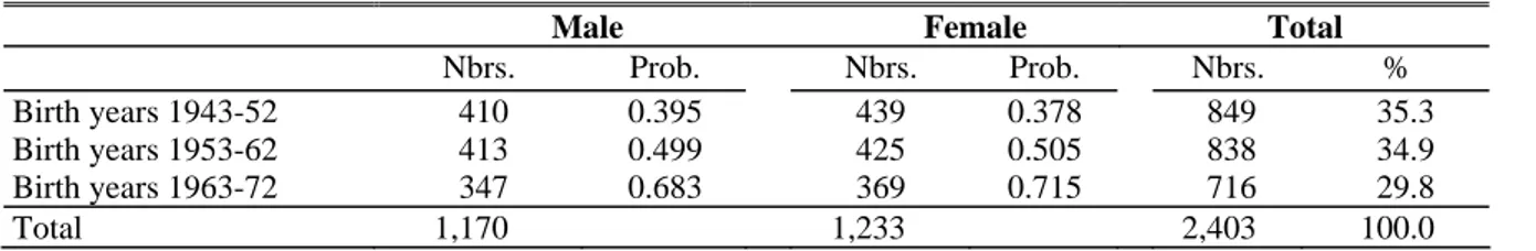
The Biomad98 survey addressed three generations of individuals: those born between 1943 and 1952 (aged 45-54 at the time of the survey), between 1953 and 1962 (35-44) and those born between 1963 and 1972 (25-34). 2,403 biographical questionnaires were collected among the individuals identified in the labour force survey, using a “grafting” technique to combine the surveys. In order to obtain a representative sample of the three generations in question, and to enable separate analysis for men and women, the main object of the study, we decided to survey around 400 people for each of the six cohorts concerned. We therefore used a survey plan stratified by generation and by gender. The distribution of the final sample by strata is given in Table 1.

Table 1 : Sample distribution by age group and sex

Male Female Total

Nbrs. Prob. Nbrs. Prob. Nbrs. % Birth years 1943-52 410 0.395 439 0.378 849 35.3 Birth years 1953-62 413 0.499 425 0.505 838 34.9 Birth years 1963-72 347 0.683 369 0.715 716 29.8

Total 1,170 1,233 2,403 100.0

Sources: Biomad98, Phase 1, 1998, MADIO, authors’ calculations. Nbrs : number of individuals. Prob.: probability of inclusion from the labour force survey.

Biomad98 presents a certain number of advantages compared with other biographical surveys in Africa (Antoine et al., 2004). The sample is larger; it is more representative and the precision of the estimators can be easily calculated. Also, the initial approach focusing on purely demographical aspects was widened to cover economic questions relating to labour market integration, following a series of nomenclatures fully harmonised with those used in the labour force survey. Finally, coupling with the labour force survey provides us with precise information on the income from the latest job. The question of income is not covered in the biographical surveys, given that it is impossible to obtain details for the whole lifetime as this is far too complex to be reliable when given in retrospective.

(11)

The matched data allows us to construct several measures of actual (rather than potential) work experience: experience off the incumbent firm or main employment, years of tenure with the current employment, in the main occupation and in the main profession.16_{Potential experience is simply age} minus years of education minus six. Actual experience is measured as months worked at the time of the Biomad98 interview and is converted into years of experience. Other labour force attachment measures include: the time spent out of the labour force (inactivity), unemployment periods, as well as the number of work interruptions over individuals’ lives, from the end of school until the date of the interview (or from the age of six if they have zero years of school attendance). This last variable is incremented by one from zero each time a spell of declared work has been interrupted by either a period of education, inactivity or unemployment. Non-working time (unemployment plus spells out of the labour force) is similarly accumulated from the age of six onwards and is calculated in years. In the rest of the paper, all these measures will be referred to as ‘labour force attachment variables’ (LFAVs).

In the data, the labour supply or paid work participation has been defined as individuals having worked at least one hour during the reference week and reporting positive earnings at the time of the interview. For those individuals who have declared positive earnings (1,928 out of 2,403 individuals), we have identified three institutional sectors of paid work participation: public wage employment, formal private wage employment and self-employment or informal sector, defined as those working in production units that are not registered or do not publish accounts.

Finally, matching these two sources of information allowed us to build a unique dataset containing biographical-type information on the individuals’ socio-economic characteristics together with a series of variables on their activity, labour incomes and job characteristics. The biographical data, spanning individuals' entire professional careers, provides relevant information that can be used to improve standard measures of human capital.

4. ECONOMETRIC METHODS 4.1. Earnings determination

4.1.1 Earnings functions and correction for selectivity

Traditional gender wage decompositions rely on estimations of Mincer-type earnings functions for men and women. Let the earning function take the usual Mincerian form:

i i i

x

w

=

β

+

ε

ln

(1)

where

ln

w

_i is the natural logarithm of the observed hourly earnings for individual i,

x

_i is a vector of observed characteristics,

β

is a vector of coefficients and

ε

_i is a disturbance term with an expected value of zero.

We estimate the log earning functions for the pooled sample and, then, separately for males and females and for the different sectors. There is no universally accepted set of conditioning variables that should be included for describing the causes of gender labour market differentials. However, the consensus is that controls for productivity-related factors such as education, experience, job tenure, marital status, presence of children, number of hours worked, union status, firm size (if available) and location of residence17_{should be included. However, it is debatable whether occupation and industry} should be taken into account: if employers differentiate between men and women through their

16_{For instance, we can distinguish the length of different types of labour market experience: the time elapsed with the same employer}

(tenure strictly speaking), the time spent in the same occupation (taking into account the fact that workers may have two different and successive occupations with the same employer), as well as the years of experience in what individuals consider as their main “profession” (e.g. a carpenter who has practised his or her main duties in different workshops or firms).

17_{In our data, this information is not particularly relevant as all individuals live in or close to the same area, that is the city of Antananarivo}

(12)

tendency to hire into certain occupations, then occupational assignment is an outcome of employer practices rather than an outcome of individual choice or productivity differences18_{. We also} incorporate in the earnings functions a dummy for formal training received during the current employment and paid by the employer. More educated workers generally receive more formal training19_{: in our sample, workers who have received formal training display, on average, 10.6 years of} schooling against 7.6 for their untrained counterparts. Besides, introducing this variable may help to control for a selection effect induced by unobserved skills of the workers, since more able employees may receive more on-the-job formal training.

Thanks to the longitudinal information available in the biographical survey, years of labour market experience, that are commonly and wrongly proxied by potential measures, are refined by using actual measures of labour market experience as well as other labour force attachment variables (LFAVs, see section 3) to take into account possible differentiated human capital depreciation (or appreciation) effects (Mincer and Ofek, 1982). Other independent variables include dummies on marital, religious and ethnic status, a dummy for the presence of a union in the current job, two dummies for the type of work contract (the reference is no contract), and the number of hours worked per week20.Sectoral and occupational dummies are also included as independent variables, but separately in the earnings decompositions, so as to propose alternative measures of the gender earnings gaps.

Since labour market participation is not likely to be random, concerns arise over possible sample selection biases in the estimations. Strictly speaking, there are two sources of selectivity bias involved. One arises from the fact that wage-earners are only observed when they work, and not everyone is working. The second comes from the selective decision to engage in public wage employment rather than private wage employment or the informal sector.

As a preliminary analysis of earnings determination between sexes, we use Heckman’s two-step procedure to deal with a possible endogeneity of the participation decision in the labour market. In the first stage, probit estimates of the probability of participation are separately performed for males and females. We then include the appropriate estimated correction term (Inverse Mill’s Ratios, IMR) into the second-stage earnings equations, for males and females respectively. The inclusion of the correction term ensures that the OLS gives consistent estimates of the augmented earnings functions. We are then able to identify a possible differentiated effect of the selection bias across gender.

The present analysis also focuses on whether the returns to observable characteristics of a wage-earner differ from one institutional sector to another. However, given the over-representation of men in the state sector, the decision to work in a particular sector may not be determined exogenously. Apart from the observed characteristics of women discussed earlier (such as education, experience or marital status), it may correlate with unobserved characteristics of the individual worker.Like Glick and Sahn (1997) or Appleton et al. (1999), we use Lee's two-stage approach to take into account the possible effect of endogenous selection in different sectors on earnings. In the first stage, multinomial logit models of individual i's participation in sector j are used to compute the correction terms,

λ

ij, from the predicted probabilities Pij. The appropriate correction term is then included in the respective earnings equation as an additional regressor in the second stage21.

In the empirical work, a multinomial logit model with four categories is then specified. It includes non-participation in paid employment (as the base category), public wage employment, formal private wage employment and self-employment or informal sector. In both Heckman’s and Lee’s procedures, identification is achieved by including various household variables (mainly drawn from the

18_{Conversely, it can be argued that analyses that omit occupation and industry may overlook the importance of background and}

choice-based characteristics on wage outcomes, while analyses that fully control for these variables may undervalue the significance of labour market constraints on wage outcomes.

19 _{See Barron, Berger and Black (1997) on this point.} 20

Other control variables were introduced, such as five dummies for the firm size in the current job, but our results were only marginally modified. We decided to omit them from the analysis in order to preserve on the degrees of freedom of our models and thus the precision of our estimates.

21_{The presence of the additional constructed selectivity correction terms renders the standard errors incorrect. White's standard errors are}

(13)

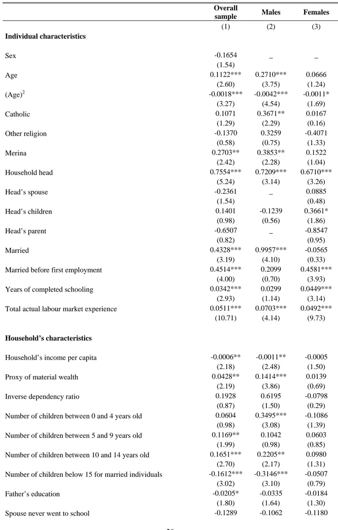
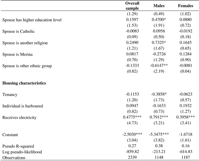
biographical survey), such as dummies for the status of the individual in the household (household head, head’s spouse, head’s children, head’s parent), the number of children by age categories (aged 0-4, 5-9 and 10-14)22_{, the household’s income per capita (without the individual’s contribution),} the inverse of the dependency ratio (number of working individuals divided by the total number of individuals in the household), a material wealth proxy23

, father and spouse’s education, spouse’s religion and ethnicity, dummies for the status of the individual vis-à-vis his/her housing (owner, tenant, harboured) and whether housing receives electricity. From the biographical data, it is also possible to test whether past events, and particularly their order of occurrence, can influence individuals’ situations with respect to the labour market at the time of the interview. For instance, we identified whether individuals were already married before getting their first job and added a dummy in the participation equations. This variable has arguably no theoretical reason to influence earnings determination but may influence employment participation, especially that of women who must balance domestic responsibilities with the need to augment family income24_{. Therefore, it appears as a} very good identifying variable for the selection equation since it is uncorrelated to the error term of the earnings equation. This is one way of overcoming the limitation of Heckman’s two-step procedure, that is, to find additional variables that arguably do affect labour market participation in the first step but have no direct impact on earnings in the second25.

4.2. Gender wage decomposition techniques

4.2.1 Oaxaca and Neumark's traditional decompositions

The most common approach to identifying sources of gender wage gaps is the Oaxaca-Blinder decomposition (e.g., Oaxaca, 1973; Blinder, 1973). Two separate standard Mincerian log wage equations are estimated for males and females. The Oaxaca decomposition is:

f f m f m m f m

w

x

w

ln

(

)

(

)

ln

−

=

β

−

+

β

−

β

(2)

where

w

m and

w

f are the means of males and females' wages, respectively;

x

m and

x

f are vectors containing the respective means of the independent variables for males and females; and

β

_m and

β

_f are the estimated coefficients. The first term on the right hand side captures the wage differential due to different characteristics of males and females. The second term is the wage gap attributable to different returns to those characteristics or coefficients.

In equation (2), the male wage structure is taken as the non-discriminatory benchmark. It can be argued that, under discrimination, males are paid competitive wages but females are underpaid. If this is the case, the male coefficients should be taken as the non-discriminatory wage structure. Conversely, if employers pay females competitive wages but pay males more (nepotism), then the female coefficients should be used as the non-discriminatory wage structure. Therefore, the issue is how to determine the wage structure

β

* that would prevail in the absence of discrimination. This choice poses the well-known index number problem given that we could use either the male or the female wage structure as the non-discriminatory benchmark. While a priori there is no preferable alternative, the decomposition can be quite sensitive to the selection made. If we let:

f

m I

β

* =Ω +( −Ω)

22 _{We also tested the proportion of children per household member but obtained less convincing results.} 23 _{The sum of the number of house, car, fridge, television, hi-fi, phone, radio and stove.}

24_{Theoretically, getting married before having a first job may raise women's opportunity costs to labour market participation and,}

therefore, their reservation wage. If it is indeed the case, the expected impact of this variable on the probability of being employed at the time of the survey should be negative (with time, their incentives to participate may be less and less important as well as their employability). However, the presence of children soon after a marriage may exert a contradictory effect since children require care and supervision, but they also increase the needs for market goods, so for labour income (for further discussions, see Glick and Sahn, 1997).

25_{The data confirms this assumption. Note the heterogeneity of the 303 individuals who got married before their first job: 73% were}

women and, at the time of the interview, 21% were no longer married, 21% were unemployed, and 16% were both no longer married and unemployed.

(14)

where Ω is a weighting matrix and I is the identity matrix, then any assumption regarding

β

* can be seen as an assumption regarding Ω. The literature has proposed different weighting schemes to deal with the underlying index problem: first, Oaxaca (1973) proposes either the current male wage structure, i.e. Ω=I (equation 2), or the current female wage structure, i.e., Ω=0 – the null matrix –, as

*

β

, suggesting that the result would bracket the “true” non-discriminatory wage structure. Reimers (1983) implements a methodology that is equivalent to Ω=0.5 I. In other words, identical weights are assigned to both men and women. Cotton (1988) argues that the non-discriminatory structure should approach the structure that holds for the larger group. In the context of sex discrimination such weighting structure implies an Ω = ImI where Im is the fraction of males in the sample.

Neumark (1988) proposes a general decomposition of the gender wage differential:

]

)

(

)

[(

)

(

ln

w

m

−

w

f

=

β

*

x

m

−

x

f

+

β

m

−

β

*

x

m

+

β

*

−

β

f

x

f (3)

This decomposition can be reduced to Oaxaca’s two special cases if it is assumed that there is no discrimination in the male wage structure, i.e.

β

*

=

β

_m, or if it is assumed that

β

* =

β

_f. Neumark shows that β* can be estimated using the weighted average of the wage structures of males and females and advocates using the pooled sample to estimate

β

*. The first term is the gender wage gap attributable to differences in characteristics. The second and the third terms capture the difference between the actual and pooled returns for men and women, respectively.

While Neumark's decomposition is attractive, it is not immune from common criticisms of decomposition methods in general, namely, the omission of variables that affect productivity. As a result, the gender wage gap may not be automatically attributed to discrimination or nepotism. Also, without evidence on the zero-homogeneity restriction on employer preferences (that is to say, employers care only about the proportion of each type of labour employed), it is not clear that the pooled coefficient is a good estimator of the non-discriminatory wage structure (Appleton et al., 1999). In addition, like other conventional decomposition methods, Neumark's decomposition fails to account for differences in sectoral structures between gender groups.

4.2.2 Appleton et al. (1999): sectoral decomposition

The decomposition technique developed by Appleton et al. (1999) takes into account sectoral structures. They adopt a similar approach to that of Neumark (1988) and decompose the gender wage gap into three components. Since this technique is based on Neumark’s decomposition, it does not suffer from the index number problem encountered by previous authors who attempted to account for differences in occupational choices in their decomposition technique (Brown, Moon and Zoloth, 1980).

Let

W

_m and W_f be the means of the natural logs of male and female earnings and

p

_mj and

p

_fj be the sample proportions of men and women in sector j respectively. Similarly to Neumark (1988), Appleton et al. (1999) assume a sectoral structure that would prevail in the absence of gender differences in the impact of characteristics on sectoral choice (p*_j, the proportion of employees in sector j under this common structure). They then decompose the difference in proportions employed in, say, three sectors (public, formal private, self-employed or informal) such as:

∑

= = = − + − + − = − 3 1 3 1 * 3 1 * * ) ( ) ( ) ( j j fj j fj j j mj mj fj mj j f m W p W W W p p W p p W (4)

(15)

A multinominal logit model is used to specify the selection process of an individual into the different sectors. If qi is a vector of i’s relevant characteristics, the probability of an employee i being in sector j is given by:

∑

= = 3 1 ) exp( / ) exp( j i ij i ij ij q q P

γ

with

i

=

m

,

f

If the distribution of men and women across sectors is determined by the same set of coefficients

γ

*j, then the probability of an employee with characteristics qi being in sector j is:

∑

= = 3 1 * * * ) exp( / ) exp( j i j i j ij q q P

γ

Hence, by estimating pooled and separate multinominal logit models for men and women, it is possible to derive the average probability for male and female employees in the different sectors. These mean probabilities are denoted by p_ij*. The relationship between

γ

* and

γ

_i are similar to that of

β

* and

β

_j in Neumark’s decomposition. Embedding the self-selection process in (4), the full decomposition can be written in the following way:

.

)

(

)

(

)

(

)

(

)

(

)

(

)

(

3 1 * 3 1 3 1 * * * 3 1 * * 3 1 3 1 * 3 1 * *

∑

= = = = = = =

−

+

−

+

−

+

−

+

−

+

−

+

−

=

−

j fj fj fj j j mj mj mj fj j fj j j mj mj j j fj j fj j j j mj mj j j fj mj j f m

p

W

p

W

p

W

p

W

x

p

x

p

x

p

W

β

(5)

The first three terms are similar to Neumark decompositions of within-sector wage gaps. The fourth and fifth terms measure the difference in earnings due to differences in distribution of male and female employees in different sectors. The last two terms account for differences in earnings resulting from the deviations between predicted and actual sectoral compositions of men and women not accounted for by differences in characteristics.

5. MADAGASCAR BACKGROUND AND DESCRIPTIVE ANALYSIS

Over the past fifteen years or so, Madagascar, one of the poorest countries in the world, has embarked on a process of economic liberalisation, similarly to many African countries undergoing structural adjustment. Over the long term, Madagascar is distinguished by a constant decline in household living standards, which in 1996 reached the lowest point since independence. From the beginning of the 1970s to 1996, per capita consumption was halved. From the mid-1990s, the reform process began to bear fruit. In 1997, growth in GDP per capita was slightly positive (+1%), for the first time in many years (Figure 1). This historic shift then accelerated, with growth reaching +4% in 2001. The contested Presidential elections in December 2001, followed by the open political crisis that continued throughout the first six months of 2002, jeopardized economic improvements, and living standards once again fell sharply (Roubaud, 2002). Since then, the country has been trying as best it can to recover.

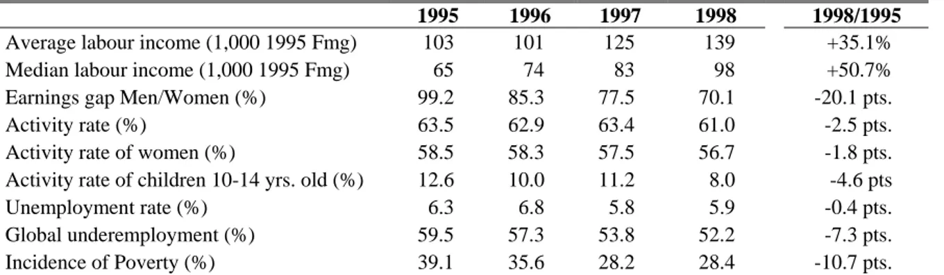
In 1998, the period referred to in this article, there had already been a very significant recovery in urban areas, especially in the capital, Antananarivo. In three years, from 1995 to 1998, the average real labour income grew by 35% and the median income by 51% (Table 2). The side-effects of growth had a very positive impact on the labour market: increase in schooling, decrease in child labour, slight decrease in unemployment, which is structurally low, but above all an end to the informal sector's domination of the labour market and a massive drop in underemployment and poverty. The incidence of extreme poverty (with the poverty line at US$ 1 in PPP) fell from 39% to 28%. In terms of gender, women's activity rate fell, corresponding to the withdrawal from the labour market of large numbers of

(16)

women who had been forced to work to provide additional income for their households during a severe crisis. At the same time, the income differential between men and women was reduced (Razafindrakoto and Roubaud, 1999).

Figure 1 : Evolution of GDP and private consumption per capita 1960-1998

Source: INSTAT, authors’ calculation.

Table 2 : Labour market dynamics 1995-1998

1995 1996 1997 1998 1998/1995

Average labour income (1,000 1995 Fmg) 103 101 125 139 +35.1% Median labour income (1,000 1995 Fmg) 65 74 83 98 +50.7% Earnings gap Men/Women (%) 99.2 85.3 77.5 70.1 -20.1 pts. Activity rate (%) 63.5 62.9 63.4 61.0 -2.5 pts. Activity rate of women (%) 58.5 58.3 57.5 56.7 -1.8 pts. Activity rate of children 10-14 yrs. old (%) 12.6 10.0 11.2 8.0 -4.6 pts Unemployment rate (%) 6.3 6.8 5.8 5.9 -0.4 pts. Global underemployment (%) 59.5 57.3 53.8 52.2 -7.3 pts. Incidence of Poverty (%) 39.1 35.6 28.2 28.4 -10.7 pts.

Sources: Enquête 1-2-3, Phase 1, 1995-1998, MADIO; authors’ calculations. The global rate of underemployment includes the three forms of underemployment: unemployment, visible underemployment (total occupied workers working for less than 35 hours against their wishes) and invisible underemployment (total workers paid less than the minimum hourly wage). The poverty line corresponds to one 1985 dollar (PPP) per capita, per day. This line was held constant in real terms for the years from 1996 to 1998 by adjusting for changes in the CPI.

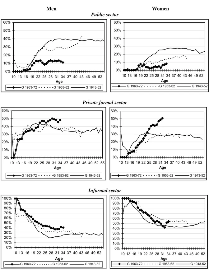
Despite improvements in the situation, the three years of recovery were not enough to erase several decades of continual deterioration in the labour market. In the long-term perspective that interests us here, the main characteristic of labour market evolution was the partial freeze on public sector recruitment from the mid-1980s, which went hand in hand with a fall in the numbers of wage-earners and an underlying rise in job precariousness. The decrease in jobs in the public sector was particularly significant for women (Antoine et al., 2000). After the age of 30, the percentage of working women present in the public sector was around 25% for the generation born between 1943 and 1952. It fell to around 10% for the intermediate generation (1953-1962) and only represented 5% for the youngest generation (Figures 2). 50 60 70 80 90 100 110 1960 1962 1964 1966 1968 1970 1972 1974 1976 1978 1980 1982 1984 1986 1988 1990 1992 1994 1996 1998 Années 100 = 196 0 PIB/Tête CONS/Tête

(17)

Figure 2 : Evolution of the job structure by cohort and gender Men Women Public sector 0% 10% 20% 30% 40% 50% 60% 10 13 16 19 22 25 28 31 34 37 40 43 46 49 52 Age G 1963-72 G 1953-62 G 1943-52 0% 10% 20% 30% 40% 50% 60% 10 13 16 19 22 25 28 31 34 37 40 43 46 49 52 Age G 1963-72 G 1953-62 G 1943-52

Private formal sector

0% 10% 20% 30% 40% 50% 60% 10 13 16 19 22 25 28 31 34 37 40 43 46 49 52 55 Age G 1963-72 G 1953-62 G 1943-52 0% 10% 20% 30% 40% 50% 60% 10 13 16 19 22 25 28 31 34 37 40 43 46 49 52 Age G 1963-72 G 1953-62 G 1943-52 Informal sector 0% 10% 20% 30% 40% 50% 60% 70% 80% 90% 100% 10 13 16 19 22 25 28 31 34 37 40 43 46 49 52 Age G 1963-72 G 1953-62 G 1943-52 0% 10% 20% 30% 40% 50% 60% 70% 80% 90% 100% 10 13 16 19 22 25 28 31 34 37 40 43 46 49 52 Age G 1963-72 G 1953-62 G 1943-52

Source : Biomad98, MADIO; Antoine et al. (2000).

Although the massive decrease in access to public jobs is common to many countries in sub-Saharan Africa, confronted since the early 1980s with a serious crisis in public finances and engaged in structural adjustment policies, the dynamism of the formal private sector since the beginning of the 1990s is, on the contrary, far more specific to Madagascar. The younger generation has the largest proportion of wage-earners in the formal private sector at the age of 25-34. This observation applies to both men and women, but is more marked for women. The phenomenon can be explained to a great extent by the spectacular growth in export processing companies in the past few years, as 80% of their

(18)

employees are young women. Finally, the formal private sector hires a growing number of members of the younger generation, in fact nearly one out of two at present.

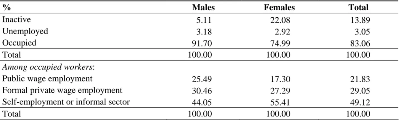
Table 3 below describes the participation and the sectoral distribution of the population across gender in 1998. The participation rate is much lower for women, while unemployment is low and not significantly different by sex. Among occupied workers, women are concentrated in low quality jobs in the informal sector. Consequently their presence in the public sector is 8 points lower than for men. Table 3 : Participation and sectoral job allocation by gender

% Males Females Total

Inactive 5.11 22.08 13.89

Unemployed 3.18 2.92 3.05

Occupied 91.70 74.99 83.06

Total 100.00 100.00 100.00

Among occupied workers:

Public wage employment 25.49 17.30 21.83 Formal private wage employment 30.46 27.29 29.05 Self-employment or informal sector 44.05 55.41 49.12

Total 100.00 100.00 100.00

Source: Enquête 1-2-3, Phase 1,1998, MADIO; authors’ calculations. Restricted to individuals between 25 and 54 years old.

Men and women bring different work experience to the labour market (Table 4). The Mincer proxy for potential work experience shows little difference in the work experience of men and women (22.6 and 24.0 years), as the average age is the same, while the average years of education (successfully completed or not) are about one year lower for women. A different story emerges when actual labour market experience is applied. The average actual work experience is 20.5 years for men compared with 17.1 years for women. A similar ratio of male to female experience appears for the actual experience off the current job and, to a lesser degree, for tenure in the current job. However, differences in the average total unemployment periods between the sexes do not seem to fully explain these disparities since males have a higher average of unemployment episodes than females. Interestingly, women display the highest average of total inactivity spells, almost twice that of men. Nonetheless, the number of work interruptions is similar across genders.

Table 4 : Differences in education and labour force attachmentfor paid work participants

Variables (in years) Males (n=1 063) Females (n=827)

Mean Std. Dev. Mean Std. Dev.

Average age 40.28 8.17 40.24 8.26 Average schooling successfully completed 8.87 4.38 7.89 4.35 Average schooling (time spent in school) 11.69 5.87 10.23 5.73 Potential work experience (age – schooling – 6) 22.60 10.24 24.01 10.72 Actual labour market experience 20.58 9.70 17.18 10.51 Actual labour market experience off the current job 11.52 9.20 9.62 9.18 Tenure with the current employer 9.24 8.43 8.08 8.05 Unemployment periods 1.14 2.18 0.82 1.90 Inactivity periods 5.52 4.12 10.84 9.44 Number of work interruptions 0.73 0.97 0.73 0.83

Sources: Enquête 1-2-3, Phase 1, 1998, Biomad98, MADIO; authors’ calculations.

Disaggregating by cohort gives a more precise view of the biases caused by only taking into account potential experience (Table 5). The bias is highest for women in the eldest generation. While the difference between potential and actual labour market experience is 4.2 years for the youngest generation of women, it increases to 11.8 for the eldest. For men, the gap is more or less constant across the cohorts (around 2 years). This result is explained by the accelerated demographic transition

(19)

process in the Madagascan capital. The number of descendants has fallen significantly in the past three decades. For example, at the age of 30, women belonging to the 1943-1952 generation had 3.4 children; at the same age, the intermediate generation only had 2.7, whereas the youngest generation has 1.8. This fall in fertility rates comes from later first births (at 25, three-quarters of women in the eldest generation had had at least one child, against barely half in the youngest generation), and also from higher intergenesic intervals, for which the median period increased from 37 months to 67 months from the eldest to the youngest generation (Antoine et al., 2000).

Table 5 : Differences in earnings and human capital across gender and generation

Variables Males Females Difference

Mean Mean

Hourly earnings* 2.20 1.52 0.68

Generation 1963-1972

Hourly earnings 1.42 0.94 0.47 Years of schooling successfully completed 9.60 9.04 0.57 Years of potential experience 10.75 11.71 -0.96 Years of actual experience 9.22 7.53 1.69

Sources: Enquête 1-2-3, Phase 1, 1998, Biomad98, MADIO; authors’ calculations. * : in Madagascan Francs (Fmg).

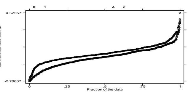
Figure 3 : Log hourly earnings of men (1) and women (2) by percentile

Figure 3 shows the log hourly earnings of men and women at each percentile of the earnings distribution. For example, the value on the vertical axis at the 50th percentile represents the median log earnings of men and women. The difference between the two curves (the surface in-between) indicates that the gender earnings gap is smaller in the upper tail of the earnings distribution and narrows throughout the distribution: low-earnings workers experience higher gender earnings inequalities than

Q ua nt ile s o f l og _ho ur ly _e ar ni ng s

Fraction of the data

1 2

0 .25 .5 .75 1

-2.78037 4.57357

(20)

high-earnings workers. This is at odds with some studies on developed countries that show the existence of a “glass ceiling” phenomenon26_.

6. ECONOMETRIC RESULTS

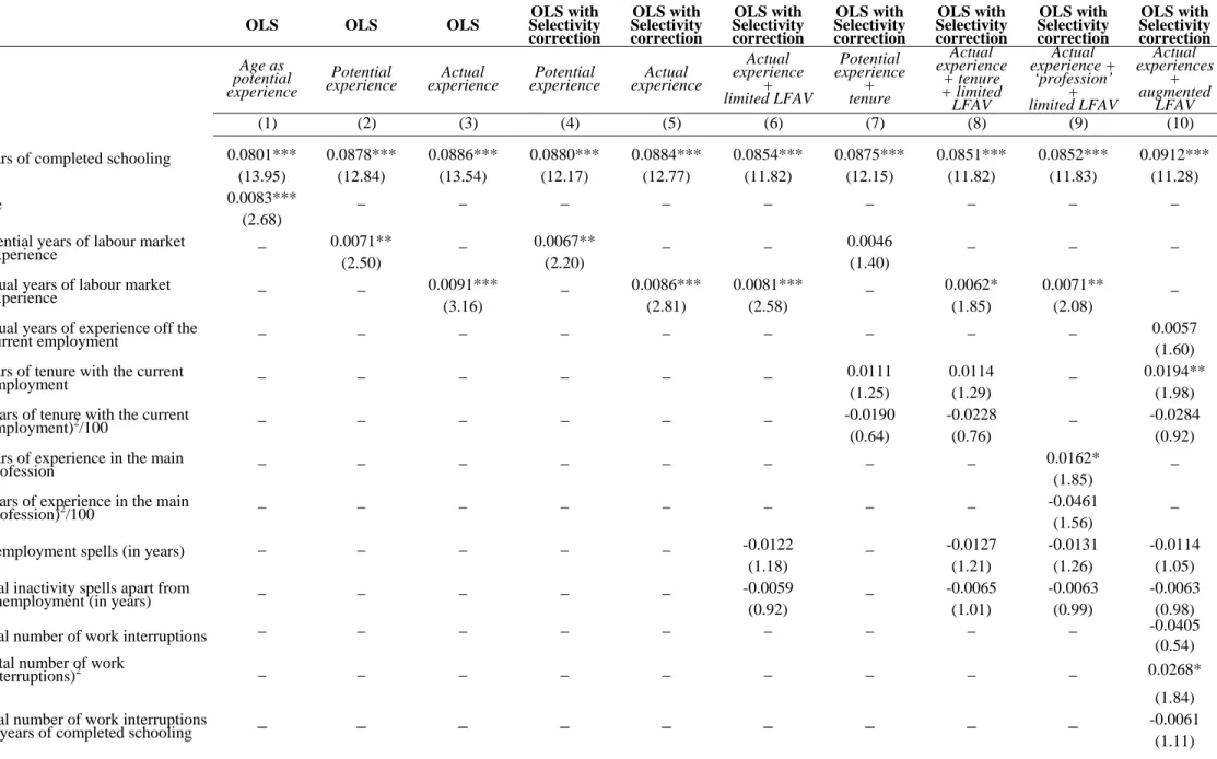
6.1. Potential versus actual experience: refining labour market attachment measures in earnings functions

Regressions introducing actual experience instead of potential experience shed light on gender-differentiated effects. From models (2) and (3), when total actual experience is accounted for, the return to experience diminishes for women while it increases for men, and becomes more significant. This is at odds with former expectations. In columns (4) and (5), the same specifications are corrected for potential selectivity bias, employing the method described in section 4.127_{. In both models, the} coefficient on the correction term (IMR) is negative and insignificant at the usual confidence interval (10% level). However, it seems to have more impact in models (4), for both men and women, that is, when actual experience is not accounted for. These results indicate that, at least when potential experience is used, the probability of having positive earnings is negatively correlated with the error terms of the earnings functions for both men and women. In other words, unobserved characteristics that increase the probability of participating in paid work may have a negative effect on earnings. Nonetheless, this mechanism of allocation in the two groups (paid work participants versus non-participants) does not affect earnings significantly.

In models (4), note that the magnitude of the coefficient on the lambda term is the same for men and women (-0.19). Interestingly, once the actual measure of experience is introduced instead of the potential one, the female correction term increases to 0.06 while it is only marginally modified for males and remains negative (column 5, Tables A1 and A2). In fact, the return to actual experience remains insignificantly modified for males after correction for potential selectivity. However, this is not the case for females for whom the actual experience variable appears somewhat underestimated without correction (columns 3 and 5, Table A2). This provides evidence that it is important to control for sample selection effects when assessing the returns to human capital, especially for women. Finally, note that the estimated marginal returns to experience are quite small and remain significantly higher for females than for males whatever the estimated model (in column 5, 1.5% against 0.8%). The latter result is a common one, especially in developing countries, given that women generally have less labour market experience than men and are therefore better rewarded for this.

Columns (6) expand the regressors of column (5) to include two labour force attachment variables (LFAVs) reflecting working time (total years of unemployment and inactivity). Adding non-working time allows for the possibility that human capital appreciates and depreciates at different rates. Inactivity is statistically significant in the female regression (at the 5% level), but insignificant in the male one. However, actual experience remains statistically significant at 1% for both sexes. Interestingly, it is men who are more likely to be penalised for unemployment, though the estimated coefficient on the unemployment variable is insignificant at 10%. Moreover, quite curiously, females show a positive premium for their periods of inactivity. This is at odds with former intuition but may be explained by socio-economic stylised facts of the Madagascan labour market and/or data deficiencies. Given the confidence we place in the quality of our data, our tentative explanation is that women’s inactivity spells are not penalised by employers because the latter may give more value to women’s home activity than to unemployment periods strictly speaking. In fact, unemployment is less likely to be related to parenting than inactivity and may voice a negative signal in employers’ eyes. In contrast, during women’s complete withdrawals from the labour market, there might be a human capital accumulation effect as a result of, for instance, childcare that provides them with parenting skills and more responsibilities in the household. As a result, women returning to work after an absence from the labour market may not necessarily suffer skill losses, nor missed promotion

26_{The existence of a glass ceiling implies that women's wages fall further behind men's at the top of the wage distribution than at the}

middle or the bottom. See Fortin and Lemieux (1998); Albrecht, Björklund and Vroman (2003) and Arulampalam, Booth and Bryan (2004).

Reassessing the Gender Wage Gap in Madagascar: Does Labour Force Attachment Really Matter?

D

OCUMENT DE

T

RAVAIL

DT/2005-06