HAL Id: tel-01099657
https://pastel.archives-ouvertes.fr/tel-01099657
Submitted on 5 Jan 2015
HAL is a multi-disciplinary open access
archive for the deposit and dissemination of
sci-entific research documents, whether they are
pub-lished or not. The documents may come from
teaching and research institutions in France or
abroad, or from public or private research centers.
L’archive ouverte pluridisciplinaire HAL, est
destinée au dépôt et à la diffusion de documents
scientifiques de niveau recherche, publiés ou non,
émanant des établissements d’enseignement et de
recherche français ou étrangers, des laboratoires
publics ou privés.
Types intersections non-idempotents pour raffiner la
normalisation forte avec des informations quantitatives
Alexis Bernadet
To cite this version:
Alexis Bernadet. Types intersections non-idempotents pour raffiner la normalisation forte avec des
informations quantitatives. Langage de programmation [cs.PL]. Ecole Doctorale Polytechnique, 2014.
Français. �tel-01099657�
´
Ecole Polytechnique
PhD Thesis
Non idempotent-intersection types
to refine strong normalisation with
quantitative information
Author: Alexis Bernadet
Jury:
Mme Simona Ronchi Della Rocca Rapporteur
Mr Lorenzo Tortora de Falco Rapporteur
Mme Mariangiola Dezani-Ciancaglini Examinateur
Mr St´ephane Lengrand Directeur de th`ese
Mr Benjamin Werner Directeur de th`ese
Mme Delia Kesner Pr´esident
Abstract
We study systems of non-idempotent intersection types for different variants of the λ-calculus and we discuss properties and applications. Besides the pure calculus itself, the variants are a calculus with explicit substitutions and a λ-calculus with constructors, matching and a fixpoint operator. The typing systems we introduce for these calculi all characterize strongly normalising terms. But we also show that, by dropping idempotency of intersections, typing a term provides quantitative information about it: a trivial measure on its typing tree gives a bound on the size of the longest β-reduction sequence from this term to its normal form. We explore how to refine this approach to obtain finer results: some of the typing systems, under certain conditions, even provide the exact measure of this longest β-reduction sequence, and the type of a term gives information on the normal form of this term. Moreover, by using filters, these typing systems can be used to define a denotational semantics.
Acknowledgements
I would like to thank St´ephane Lengrand, Benjamin Werner, Mariangiola Dezani-Ciancaglini, Delia Kesner, Simona Ronchi Della Rocca, Lorenzo Tortora de Falco, David Monniaux, Thierry Coquand, Philippe Chassignet, Benjamin Smith, Sylvie Putot, Julie Bernauer, Jean Goubault-Larrecq, Paul-Andr´e Melli`es, Pierre-Louis Curien, Alain Prout´e and my family.
Contents
Acknowledgements . . . 1
1 Introduction 4 1.1 Generalities . . . 4
1.2 About the λ-calculus . . . 7
1.3 Brief description of the Chapters . . . 8
1.4 Introduction to α-equivalence . . . 9
2 A simple typing system of non-idempotent intersection types for pure λ-calculus 12 2.1 Introduction. . . 12
2.2 Syntax and operational semantics. . . 13
2.3 The typing system . . . 14
2.3.1 Types . . . 14
2.3.2 Contexts . . . 16
2.3.3 Rules . . . 17
2.4 Soundness . . . 18
2.5 Semantics and applications . . . 20
2.5.1 Denotational semantics . . . 20
2.5.2 Example: System F . . . 24
2.6 Completeness . . . 26
2.7 Conclusion . . . 33
3 Intersection types with explicit substitutions 35 3.1 Introduction. . . 35
3.2 Syntax . . . 35
3.3 Typing judgments . . . 37
3.4 Soundness . . . 38
3.5 Special property of typing trees: Optimality . . . 38
3.6 Completeness . . . 39
3.7 Complexity . . . 42
3.8 Conclusion . . . 43
4 A big-step operational semantics via non-idempotent intersection types 45 4.1 Introduction. . . 45
4.2 Basic definitions and properties . . . 47
4.2.1 Syntax. . . 47
4.2.2 Intersection types and contexts . . . 49
4.2.3 Typing system . . . 51
4.3 Characterisation of the typing system . . . 53
4.3.1 Soundness . . . 53
4.4 Refined soundness . . . 55
4.4.1 Complexity . . . 55
4.4.2 Viewing optimal typing as a big-step semantics . . . 56
4.5 Alternative systems. . . 58
4.5.1 Variant with no information about the normal form . . . 58
4.5.2 Obtaining the exact normal form . . . 58
4.6 Conclusion . . . 59
5 Strong normalisation in a calculus with constructors and fixpoints via non-idempotent intersection types 60 5.1 Introduction. . . 60
5.2 Calculus . . . 62
5.2.1 Definition of the calculus . . . 62
5.2.2 Refined notion of reduction . . . 64
5.3 Strong normalisation . . . 68 5.3.1 Intersection types. . . 69 5.3.2 Soundness . . . 71 5.3.3 Completeness . . . 71 5.4 Conclusion . . . 72 5.5 Confluence . . . 72 5.6 Example in Caml . . . 74 6 Conclusion 75 A Full proofs 80 B A simple presentation of de Bruijn indices 102 B.1 Definitions. . . 102
B.2 Binding . . . 102
B.3 Substitutions . . . 104
B.4 β-reduction . . . 106
Chapter 1
Introduction
1.1
Generalities
What is a programming language ? A programming language is a set of
sequences of symbols where each of these sequences describes more or less an action or a computation. Such sequence of symbols is called a program of this programming language. It is needed to build computer software. For real world programs, these sequences of symbols are written in one or more files in the computer.
The most obvious programming language is the machine language which can be directly interpreted by a computer. There are two main reasons why most software are not written in the machine language:
• It is really hard to write anything with it, even small programs.
• There exists a different machine language for each computer architecture. Therefore, we may need to rewrite the entire program if we want to port it on an different platform.
Therefore, almost every other software are written in programming languages that are more human readable, more scalable, more portable, more machine-independent and, sometimes, safer. Programs written in these languages cannot be directly interpreted by a computer.
• There can be a software that transforms a program written in some language to a program written in the machine language. This software is called a compiler.
• There can be a software that interpret a program written in some language and do what the program is supposed to do. This is called an interpreter. Of course, things can be a little more complicated than that:
• A program in some language can be compiled to another language which is not the machine language and, to be executed, the new program obtained requires an interpreter.
• Compilation can be in several steps: the program can be written in several intermediate languages until we reach the target language. This is useful when creating a programming language and its compiler to not have to worry about technical problems that have already been solved by more competent people. Solving these problems ourselves may be called reinventing the wheel. For examples, lots of high-level programming language are compiled to a language called C. Most compiler can compile C to assembler which is a programming language that is just above the machine language in terms of abstraction. Finally, the assembler program can be compiled to machine language and then, we can execute it. Therefore, if someone wants to write the compiler of
a new high-level language, they just have to be able to compile it to C, and then they can have quite fast executables.
When writing a program, someone might wonder what its meaning is or what it does. We usually have these two approaches:
• We give an intuitive meaning to each construction of the language. The meaning given is not very different from what someone would have written if we were trying to explain in a tutorial or a lesson what a construction does. Of course, this has no mathematical value.
• We say that the meaning of a program is what it does when executed (af-ter compilation if any). This is also not usually suited to do mathematical reasoning on programs.
Therefore, if we want to have mathematical results about programs (such as cor-rectness), we need to define formally the meaning of a program. This is called the semantics of a programming language. Ensuring the correctness of a program is useful when there are lives as stake (programs in a plane, etc. . . ) or even when there is money at stake (for example, the crash of a program used in a bank). Even when it is just saving debugging time (time spent searching and correcting mistakes that occurs during the execution of a program) it is well worth it. There are two main approaches:
• The operational semantics: There are syntactic rules (usually reduction rules) that describe what a program does. In some ways, it is paraphrasing the interpreter.
• The denotational semantics: We create a mathematical object and we use it as a model of the programming language: A program is interpreted as “something” in this mathematical object (for example, it can be an element of a set or a morphism in a category). For a given programming language, there are usually lots of possible models.
The difference between these two is similar to the difference between “what it is” (denotational semantics) and “what it does” (operational semantics).
When studying semantics, we usually start with a minimalistic/toy language. Most of the time, when we are complexifying the language we can easily extend and adapt the definitions, results and proofs. The λ-calculus is one of the most well known minimalistic languages.
Also, when working with terms and programs, we prefer to work with an ab-stract expression tree instead of a sequence of symbols. For example, the following sequence of 7 symbols:
3 × (4 + 5)
can be transformed into the following abstract expression tree:
3
4 5
+ ×
Even if we are manipulating abstract expression trees, we usually write them in one line (in the above example we write 3×(4+5)). Transforming a sequence of symbols to an abstract expression tree is done by something called a lexer and another thing called a parser. Usually, when working on semantics we ignore this aspect.
What is typing in a programming language ?
Originally, types are used in a programming language as an indication for the compiler about how to represent data. For example, an integer (which has type “int”) has not the same representation as a floating number (which has type “float”). As computers got faster, a certain number of programming languages (and quite a few of them, like Python, became popular), choose to get rid of the types in the
language. This leads to a small cost at runtime (we need to keep information about the types) in exchange of the possibility to write shorter programs.
On the other side, some people (such as the developers of the ML family of programming languages) consider that having information about the types at com-pilation time is a bonus because it makes the catching of mistakes at comcom-pilation time easier.
The argument that not having types makes programs shorter to write is not necessary valid: a compiler can try to guess the types in a program. This is called typing inference. Hence, we have the best of both worlds. Actually, the more the types are expressive, the harder it is to infer them. For example, Girard’s System F cannot be inferred [Wel96]. Moreover, most of the systems using intersection types[CD78], such as the ones studied in this thesis cannot be inferred.
What is logic ?
Set Theory has imposed itself as the main language for doing mathematics. How-ever, at the beginning of the 20th century, mathematicians realized that certain rea-soning with sets could lead to contradictions (for example, Russel’s paradox [vH02]: the set of all the sets is not a set).
Therefore, it seemed necessary to sanitize the mathematical foundations: decid-ing what was a valid (or sound) proof and what was not. Of course, to do this, we need to give a mathematical definition of a proof.
Such proofs can be represented in a computer. Hence, we can write a Proof Assistant: we write a proof in a computer, and the Proof Assistant checks whether or not the proof is sound. Also, the writing of some parts of the proofs can be automated.
What is intuitionistic logic ?
Alan Turing proved [Tur36] that some functions (defined mathematically) could not be calculated by a computer. It is not a question of time or memory available. It turns out that the reason we are in this situation is that we can use in mathematics the principle of excluded middle (for every formula A, A is true or the negation of A is true). By dropping excluded middle we we are in a new logic called intuitionistic logic and when we have excluded middle we says that we are in classical logic. The idea of intuitionistic logic is from Brouwer [vH02] and has been developed by Heyting [Hey71]. One of the most modern way of defining intuitionistic logic is Topos Theory: an Lawvere’s Elementary Topos [LS09] can be used as a model of intuitionistic logic. On the one hand, we can prove fewer theorems in intuitionistic logic (compared to classical logic). On the other hand:
• A definition (resp. theorem) that is used (resp. holds) in classical logic might not be intuitionistically friendly (resp. be proved in intuitionistic logic). How-ever, it may be possible to have a definition (resp. theorem) that is equivalent in classical logic but is also intuitionistically friendly (resp. holds in intuition-istic logic) and not more complicated than the original one.
• When something is proved in intuitionistic logic it gives more information than in classical logic: the proof is constructive. In particular, if we can define a function in intuitionistic logic, then this function is computable. This is the reason intuitionistic logic is also called constructive logic.
Moreover, we can find a correspondence between intuitionistic proofs and functional programs: This is called the Curry-Howard correspondence [GLT89].
What is linear logic ?
When a program runs, resources (data in memory) can be duplicated or erased. It is possible to have a calculus/programming language that has restrictions on duplicating/erasing resources. By interpreting this through the Curry-Howard cor-respondence, we can build a corresponding logic where we have restrictions on using a proof several times or not using it at all: This is called linear logic and it was
invented by Girard [GLT89]. One particularity of linear logic, is that we have two “and” and two “or”. Linear logic is strongly related to the topic of this thesis, namely the idea of using intersection types that are not idempotent (A ∩ A is not equivalent to A, see the next section).
1.2
About the λ-calculus
The λ-calculus is a minimalistic programming language created by Church [Chu85]. In this programming language there is no distinction between programs and data. A program M in the pure λ-calculus is called a λ-term and is either:
• A variable x, y, z, . . .
• An abstraction of the form λx.M . Intuitively, λx.M describes the function that maps x to M . For example, λx.x is the identity function.
• An application of the form M N where M is the function and N is the argu-ment.
The fact that this programming language looks simplistic can be balanced as follows: • It is possible to encode in this calculus, usual data structures (such as booleans, integers, lists, trees, etc . . . ) and more advanced constructions. For exam-ple, the integer n is encoded as the λ-term λf.λx.fnx (with f0x = x and
fn+1x = f (fnx)). We can also encode recursion and then prove that the
λ-calculus is Turing complete: anything that can be “computed” can be written in λ-calculus. This is both a blessing and a curse.
• It is possible to enrich the λ-calculus with usual data structures and more advanced constructions expressed as new primitives of the language rather as encodings. Most definitions, theorems and proofs of the λ-calculus without this enrichment (also called the pure λ-calculus) can be adapted. By taking a step further, we can design real world programming languages based on the λ-calculus. These languages are called functional programming languages. OCaml and Haskell are among those.
The syntax of λ-calculus is very simple, but we still have to define what a λ-term formally means. This is defining the semantics of the λ-calculus. The main idea is that (λx.M )N has the same meaning as M {x := N } where M {x := N } is M where we “replaced every x in M by N ”. Moreover, going from (λx.M )N to M {x := N } is a step in the computation. An occurrence (λx.M1)M2inside a term
M is called a β-redex; and replacing an occurrence of (λx.M1)M2by M1{x := M2}
is called a β-reduction. When we cannot do any β-reduction, the computation is over and the term M that cannot be reduced is the result of the computation. If from a term M we can reach a term M0 that cannot be reduced, then M0 is called the normal form of M .
When defining this semantics formally, several questions and problems arise: • We have to formally define what the term M {x := N }.is. The definition is
quite subtle and relies on an equivalence relation that identifies some terms (like λx.x and λy.y which both describe the identity function). This relation is called α-equivalence. Usually, λ-terms are considered modulo α-equivalence. The easiest way of defining and manipulating this equivalence is probably by using nominal logic techniques (see Section1.4).
• If there are several β-redexes in a term M , then there are several ways of doing a β-reduction. Therefore, the normal form does not seem to always be unique. Actually, it is unique, and it is a corollary of the confluence property: If M can reach M1 and M can reach M2 then there exists M3 such that M1
and M2 can reach M3. It is possible to prove confluence by using something
called parallel reductions [CR36].
• The question about whether or not the normal form exists: Some λ-terms do not have a normal form. For example, (λx.xx)(λx.xx) can only reduce to itself. By the fact that the λ-calculus is Turing complete, we cannot avoid the fact that the computation of some terms does not terminate and we cannot even decide by a program if a term does terminate or not (that would give a solution to the Halting Problem and contradict Turing’s result[Tur36]). Even when the normal form exists, by the fact that a λ-term can be reduced several ways, we can consider the two following cases:
– There exists a β-reduction sequence to the normal form. This is called weak normalisation.
– We do not have an infinite β-reduction sequence: Any β-reduction strat-egy terminates. This is called strong normalisation. By the fact that a λ-terms has a finite number of β-redexes, strong normalisation of M is equivalent to having a longest reduction sequences from M .
For example, (λy.z)((λx.xx)(λy.xx)) (with y 6= z) is weakly normalising (the normal form is z) but is not strongly normalising (it reduces to itself). In this thesis, we are more interested in the strong normalisation property.
We have described the operational semantics of the λ-calculus. It is also possible to give a devotional semantics. For example, we can interpret each λ-term as an element of a Scott Domain [Sco82a] (which is a partially ordered set that satisfies some properties).
If we want to easily manipulate λ-terms and ensure they have some properties (such as strong normalisation), we can use types. If M has some type A (written M : A) then, by a Soundness Theorem, we can prove that M has some properties described by A. The typing judgment is defined with induction rules.
The most basic typing system for λ-calculus are the simple types where a type is either a constant τ or an arrow A → B. If we have M : A → B, it means that M is a “function” that goes from A to B. The main idea is that:
• If M : A → B and N : A, then M N : B. • If M : B with x : A, then λx.M : A → B.
Actually, more formally, the typing judgments are of the form Γ ` M : A where Γ is something called a context and indicates the type of each variables in M . Simple types have the following interesting property: If M is typable, then M is strongly normalising.
It is possible to enrich the types with an intersection construction: If A is a type and B is a type, then A ∩ B is a type. The main idea is that if M : A and M : B, then M : A ∩ B. Usually, we have an equivalence relation ≈ on types (to have associativity, commutativity of intersection etc . . . ). We also usually have A ∩ A ≈ A: the intersection is idempotent.
In most of the thesis, we are going to drop the idempotency of intersection and we are going to see how it can give more information about quantitative properties on a λ-term: If M : A ∩ A, then M will be used twice as a program of type A.
1.3
Brief description of the Chapters
In Chapter 2,we define a typing system for pure λ-calculus. The types used in this system are intersection types: If M is of type A and M is of type B, then M is of a type written A ∩ B. The particularity of this typing system is that the intersection is not idempotent: A ∩ A is not the same as A. This leads to various
properties and applications that we study: First, similarly to the case of idempotent intersection types, this typing system characterizes strongly normalising terms: a term is typable if and only if it is strongly normalising. Also, we can use this typing system to define a denotational semantics of λ-calculus where values are filters of types. This semantics can serve as a tool to prove strong normalisation in other typing systems. We illustrate this with the example of System F. Finally, we have a complexity result: A trivial measure on a typing tree of a term M gives us an upper bound on the size of the longest β-reduction sequences from M .
The complexity result obtained in Chapter2 is an inequality result. We would rather have an equality result, extracting from the typing tree of a term the exact size of the longest reduction sequences. For this, in Chapter 3 we refine the λ-calculus: Instead of the pure λ-calculus, we work with λS which is a λ-calculus with explicit substitutions M [x := N ]. In this calculus the erasure of a sub-term can be postponed and this simplifies the study of various results. In particular, we extract from typing trees the exact size of the longest reduction sequences, defined in terms of its number of B-steps ((λx.M )N →B M [x := N ]) rather than β-steps (which are not primitive reductions of this calculus). Moreover, for this improved complexity result, we have to restrict ourselves to certain types of typing trees that we call “optimal”.
In Chapter 4, we also refine the complexity result of Chapter 2, but still for the pure λ-calculus (unlike Chapter3). However, we now use an enriched grammar for types and we add extra rules to the typing system. This typing system still characterises strongly normalising normal terms and has its own definition of an optimal typing tree; these optimal typing trees provide the exact size the longest β-reduction sequences and can be considered as the derivation of a big-step operational semantics. In particular types describe the structure of normal forms.
In Chapter 5, we extend the typing system of Chapter2 to a calculus that is closer to a real world programming language. In particular, this calculus provides constructors and matching to easily use algebraic data types, and a fixpoint operator to write recursive functions. As in the previous chapters, a term is typable if and only if it is strongly normalising.
The chapters can almost be read mostly independently. but we recommended to read Chapter2 before the other ones.
This thesis is written in the implicit framework of classical set theory (ZFC) with first order logic; however when we work with λ-terms (of the various calculi), we consider them up to α-equivalence. In Section 1.4, we are going to show what this formally means for the pure λ-calculus. We will not explicitly develop these technical points for the other calculi handled in this thesis (other we could), but we will only write “we consider terms up to α-equivalence”.
1.4
Introduction to α-equivalence
In this section we show how α-equivalence can be formally defined in the framework of the pure λ-calculus. The main idea is that α-equivalence is defined by using permutations and is inspired by nominal logic [Pit03].
Assume we have an infinite (countable) set Var. Definition 1 (Permutations).
A permutation π is a bijection from Var to Var such that Dom(π) defined by: Dom(π) := {x ∈ Var | π(x) 6= x}
is finite.
Perm is the set of the permutations and forms a group:
x ≈αx M ≈αM0 N ≈αN0 M N ≈αM0N0 π ∈ Perm π(x) = y π.M ≈αM0 fv(M ) ∩ Dom(π) ⊆ {x} λx.M ≈αλy.M0 (λ) Figure 1.1: α-equivalence
For all π1, π2∈ Perm, π2◦π1defined by (π2◦π1)(x) = π2(π1(x)) is a permutation
and (π1π2)−1 = π2−1π −1
1 and Dom(π2◦ π1) ⊆ Dom(π1) ∪ Dom(π2).
For all x, y ∈ Var, < x, y > defined by: < x, y > (x) = y < x, y > (y) = x
< x, y > (z) = z (z 6= x, z 6= y)
is a permutation and < x, y >−1=< x, y > and Dom(< x, y >) = {x, y}. Moreover, < x, y >=< y, x >.
Definition 2 (λ-terms and α-equivalence).
λ-terms are defined with the following grammar:
M, N ::= x | λx.M | M N
x ∈ Var
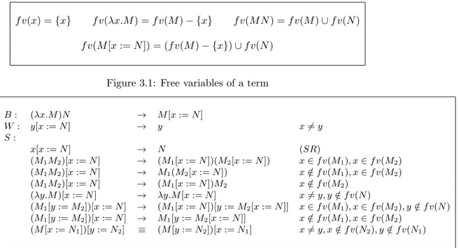
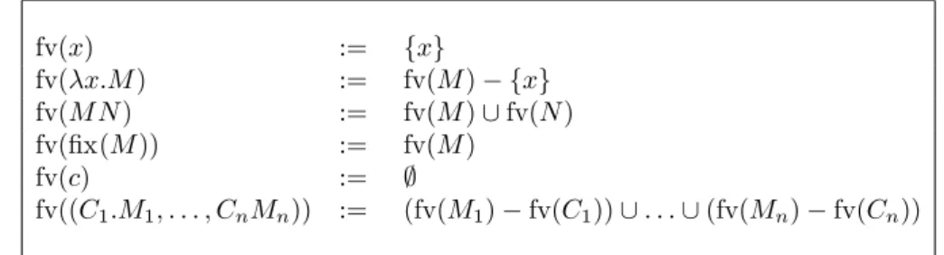
Free variables of M is a finite set of variables defined by induction on M as follows:
fv(x) := {x}
fv(M N ) := fv(M ) ∪ fv(N )
fv(λx.M ) := fv(M ) − {x}
The action of π on M is defined by induction on M as follows:
π.x := π(x)
π.(M N ) := π.M π.N
π.(λx.M ) := λπ(x).π.M
The size of a term M is defined by induction on M as follows:
|x| := 1
|M N | := |M | + |N |
|λx.M | := |M | + 1
α-equivalence is defined with the rules of Figure1.1. In rule (λ) the permutation π is a witness of the α-equivalence.
Lemma 1 (Properties of λ-terms).
1. id.M = M and π2.π1.M = (π2◦ π1).M . 2. fv(π.M ) = {π(x) | x ∈ fv(M )}. Therefore if x ∈ fv(π.M ), then π−1(x) ∈ fv(M ). 3. If M ≈αM0 then π.M ≈απ.M0, fv(M ) = fv(M0) and |M | = |M0|. 4. If M ≈αM0, then λx.M ≈αλx.M0. 5. ≈α is an equivalence relation.
6. If for all x ∈ fv(M ), π(x) = x, then M ≈απ.M .
7. If for all x ∈ fv(M ), π1(x) = π2(x), then π1.M ≈απ2.M
8. If x 6= y and y /∈ fv(M ) and < x, y > .M ≈αM0, then λx.M ≈αλy.M0.
10. If λx.M ≈αλy.M0 and x 6= y, then y /∈ fv(M ) and < x, y > .M ≈αM0.
Proof. 1. By induction on M .
2. By induction on M .
3. By induction on M ≈αM0. Only one case is not trivial: We have λx.M1≈α
λy.M2 with π1 as a witness. We then prove that λπ(x).π.M1≈αλπ(y).π.M2
with the rule (λ) and the permutation π ◦ π1◦ π−1 as witness.
4. We use rule (λ) with the permutation id.
5. • We prove reflexivity by induction on M . For the λx.M1case, we use the
item 4.
• We prove symmetry by induction on M ≈αM0. For the (λ) rule with π
as a witness of λx.M1≈αλy.M2, we use π−1 as a witness of λy.M2≈α
λx.M1.
• We prove transitivity by induction on M1 that if M1≈αM2and M2≈α
M3, then M1≈αM3. There is only one case that is not trivial: We have
λx.M1≈αλy.M2 with π1 as a witness and λy.M2≈αλz.M3 with π2 as
a witness. We use π2◦ π1as a witness of λx.M1≈αλz.M3.
In particular, we have π1.M1 ≈α M2 and π2.M2 ≈α M3. Therefore,
M1 ≈απ−1.M2 and π1−1.M2≈α π1−1.π −1 2 .M3. By induction hypothesis on M1, we have M1≈απ1−1.π −1 2 M3. Hence (π2◦ π1).M1≈αM3.
6. By induction on M . In particular, for λx.M1, we use the rule (λ) with π as a
witness.
7. For all x ∈ fv(M ), we have π1(x) = π2(x). Hence, (π2−1◦π1)(x) = π2−1(π1(x)) =
x. By item 6, we have (π2−1◦ π1).M ≈αM . Therefore, π1.M ≈απ2.M .
8. We use the rule (λ) with < x, y > as a witness. 9. Corollary of item 6.
10. Corollary of item 7.
Lemma1.5 allows us to quotient the grammar of λ-terms by α-equivalence; more generally the properties will be used implicitly throughout the thesis.
In the rest of the thesis, the work concerning α-equivalence, even for other calculi, is assumed and terms are considered up to α-equivalence.
Another possibility is to work with De Bruijn indices and then we do not have to define the α-equivalence. However, the proofs and formalism are heavier. A glimpse on how to work with De Bruijn is given in AppendixB. It would have been possible to write this thesis with De Bruijn indices.
Chapter 2
A simple typing system of
non-idempotent intersection
types for pure λ-calculus
2.1
Introduction
Intersection types were introduced in [CD78], extending the simply-typed λ-calculus with a notion of finite polymorphism. This is achieved by a new construct A ∩ B in the syntax of types and new typing rules such as:
M : A M : B
M : A ∩ B where M : A denotes that a term M is of type A.
One of the motivations was to characterise strongly normalising (SN) λ-terms, namely the property that a λ-term can be typed if and only if it is strongly normalis-ing. Variants of systems using intersection types have been studied to characterise other evaluation properties of λ-terms and served as the basis of corresponding semantics [Lei86, Ghi96,DCHM00,CS07].
This chapter refines with quantitative information the property that typability characterises strong normalisation. Since strong normalisation ensures that all re-duction sequences are finite, we are naturally interested in identifying the length of the longest reduction sequences. We do this with a typing system that is very sensitive to the usage of resources when λ-terms are reduced.
This system results from a long line of research inspired by Linear Logic [Gir87]. The usual logical connectives of, say, classical and intuitionistic logic, are decom-posed therein into finer-grained connectives, separating a linear part from a part that controls how and when the structural rules of contraction and weakening are used in proofs. This can be seen as resource management when hypotheses, or more generally logical formulae, are considered as resource.
The Curry-Howard correspondence, which originated in the context of intu-itionistic logic [How80], can be adapted to Linear Logic [Abr93, BBdH93], whose resource-awareness translates to a control of resources in the execution of programs (in the usual computational sense). From this, have emerged some versions of lin-ear logic that capture pastime functions [BM03,Laf04, GR07]. Also from this has emerged a theory of λ-calculus with resource, with semantical support (such as the differential λ-calculus) [ER03, BEM10].
(λx.M )N →β M {x := N } M →βM0 λx.M →βλx.M0 M →βM0 M N →βM0N N →βN0 M N →βM N0 Figure 2.1: β-reduction
of reduction lengths in the λ-calculus by means of non-idempotent intersection types (as pioneered by [KW99,NM04]).
Intersections were originally introduced as idempotent, with the equation A ∩ A = A either as an explicit quotient or as a consequence of the system. This corresponds to the understanding of the judgement M : A ∩ B as follows: M can be used as data of type A or data of type B. But the meaning of M : A ∩ B can be strengthened in that M will be used once as data of type A and once as data of type B. With this understanding, A ∩ A 6= A, and dropping idempotency of intersections is thus a natural way to study control of resources and complexity. Using this, de Carvalho [dC09] has shown a correspondence between the size of the typing derivation tree and the number of steps taken by a Krivine machine to reduce the term. This relates to the length of linear head-reductions, but if we remain in the realm of intersection systems that characterise strong normalisation, then the more interesting measure is the length of the longest reduction sequences. In this chapter we get a result similar to de Carvalho’s, but with the measure corresponding to strong normalisation.
In Section 2.2 we formally give the syntax and operational semantics of the λ-calculus. In Section 2.3, we define a system with non-idempotent intersection types. In Section2.4, we prove that if a term is typable then it is SN (soundness). In Section2.5, we use the typing system to define a denotational semantics and we show examples of applications. In Section 2.6, we prove that if a term is strongly normalising then it is typable.
2.2
Syntax and operational semantics
In this section we formally give the syntax and operational semantics of the λ-calculus.
Definition 3 (λ-terms). Terms are defined in the usual way with the following grammar:
M, N ::= x | λx.M | M N
Free variables fv(M ) and substitutions M {x := N } are defined in the usual way and terms are considered up to α-equivalence.
The notion of reduction is the usual β-reduction:
Definition 4 (β-reduction). M →β M0 is defined inductively by the rules of Fig-ure 2.1.
To make some proofs and theorems about strong normalisation more readable, we use the following notations:
Definition 5 (Strongly normalising terms). Assume n is an integer. We write SN for the set of strongly normalising terms for →β.
F ≈ F A ∩ B ≈ B ∩ A (A ∩ B) ∩ C ≈ A ∩ (B ∩ C) A ∩ (B ∩ C) ≈ (A ∩ B) ∩ C A ≈ A0 B ≈ B0 A ∩ B ≈ A0∩ B0 ω ≈ ω A ≈ B B ≈ C A ≈ C Figure 2.2: Equivalence between types
We write SN=n for the set of strongly normalising terms for →β such that the
length of longest β-reduction sequences is equal to n. The set SN≤n is defined by:
SN≤n:= Sm≤nSN=m
2.3
The typing system
In Section 2.3.1, we define the intersection types. In Section 2.3.2, we define con-texts. In Section2.3.3, we define the typing system and give basic properties.
2.3.1
Types
In this chapter, intersection types are defined as follows:
Definition 6 (Intersection types).
F -types, A-types and U -types are defined with the following grammar:
F, G ::= τ | A → F
A, B, C ::= F | A ∩ B
U, V ::= A | ω
where τ ranges over an infinite set of atomic types.
With this grammar, U ∩ V is defined if and only if U and V are A-types. Therefore, by defining A ∩ ω := A, ω ∩ A := A and ω ∩ ω := ω, we have U ∩ V defined for all U and V .
Some remarks:
• The property that, in an arrow A → B, B is not an intersection, is the standard restriction of strict types [vB95] and is used here to prove Lemma5.1. • ω is a device that allows synthetic formulations of definitions, properties and proofs: U types are not defined by mutual induction with Atypes and F -types, but separately, and we could have written the chapter without them (only with more cases in statements and proofs).
For example, (τ → τ ) ∩ τ is an A-type.
To prove Subject Reduction and Subject Expansion (Theorems 1 and 5) by using Lemmas6 and12, we have to define equivalence ≈ and inclusion ⊆ between types. Here is the formal definitions and basic properties (notice that we do not have A ≈ A ∩ A):
Definition 7 (Equivalence between types).
Assume U and V are U -types. We define U ≈ V with the rules given in Fig-ure 2.2.
The fact that ≈ is an equivalence relation can be easily proved (Lemma2.4). Therefore, adding rules for reflexivity, symmetry and transitivity is superfluous and
only adds more cases to treat in the proofs of statements where such a relation is assumed (e.g. Lemma 5.2).
Lemma 2 (Properties of ≈).
1. Neutrality of ω: U ∩ ω = ω ∩ U = U .
2. Strictness of F -types: If U ≈ F , then U = F . 3. Strictness of ω: If U ≈ ω, then U = ω. 4. ≈ is an equivalence relation.
5. Commutativity of ∩: U ∩ V ≈ V ∩ U
6. Associativity of ∩: U1∩ (U2∩ U3) ≈ (U1∩ U2) ∩ U3
7. Stability of ∩: If U ≈ U0 and V ≈ V0, then U ∩ V ≈ U0∩ V0.
8. If U ∩ V = ω, then U = V = ω. 9. If U ∩ V ≈ U , then V = ω. Proof. 1. Straightforward. 2. By induction on U ≈ F . 3. Straightforward. 4.
• Reflexivity: We prove that U ≈ U by induction on U .
• Symmetry: We prove by induction on U ≈ V that if U ≈ V , then V ≈ U . • Transitivity: Straightforward.
5. Straightforward. 6. Straightforward. 7. Straightforward. 8. Straightforward.
9. For all U , we construct ϕ(U ) defined by induction on U as follows:
ϕ(F ) := 1
ϕ(A ∩ B) := ϕ(A) + ϕ(B)
ϕ(ω) := 0
By induction on U , if ϕ(U ) = 0, then U = ω We also have ϕ(U ∩ V ) = ϕ(U ) + ϕ(V ).
By induction on U ≈ V , if U ≈ V , then ϕ(U ) = ϕ(V ).
If U ∩ V ≈ U : Then, ϕ(U ∩ V ) = ϕ(U ). Therefore, ϕ(U ) + ϕ(V ) = ϕ(U ). Hence, ϕ(V ) = 0. Therefore, V = ω.
Definition 8 (Sub-typing).
Assume U and V are U -types. We write U ⊆ V if and only if there exists a U -type U0 such that U ≈ V ∩ U0.
Lemma 3 (Properties of ⊆).
1. ⊆ is a partial pre-order and ≈ is the equivalence relation associated to it: U ⊆ V and V ⊆ U if and only if U ≈ V .
3. Stability of ∩: If U ⊆ U0 and V ⊆ V0, then U ∩ V ⊆ U0∩ V0.
4. Greatest element: U ⊆ ω.
Proof. Straightforward.
We could have represented intersection types with multisets (and correspond-ingly used the type inclusion symbol ⊆ the other way round). We chose to keep the standard notation A ∩ B, with the corresponding inclusion satisfying A ∩ B ⊆ A, since these are interpreted as set intersection and set inclusion in some models (e.g. realisability candidates). This way, we can also keep the equivalence relation explicit in the rest of the chapter, which gives finer-grained results. For example, the equivalence only appears where it is necessary and the proof of Lemma 5.2 shows the mechanism that propagates the equivalence through the typing trees. These presentation choices are irrelevant to the key ideas of the chapter.
2.3.2
Contexts
To define typing judgements (Definition 10), we need to define contexts and give their basic properties. We naturally define pointwise the notion of equivalence and inclusion for contexts. More formally:
Definition 9 (Contexts).
A context Γ is a total map from the set of variables to the set of U -types such that the domain of Γ defined by:
Dom(Γ) := {x | Γ(x) 6= ω} is finite.
∩, ≈ and ⊆ for contexts are defined pointwise:
(Γ ∩ ∆)(x) := Γ(x) ∩ ∆(x)
Γ ≈ ∆ ⇔ ∀x, Γ(x) ≈ ∆(x)
Γ ⊆ ∆ ⇔ ∀x, Γ(x) ⊆ ∆(x)
Notice that if Dom(Γ) and Dom(∆) are finite, then Dom(Γ ∩ ∆) is finite. Therefore Γ ∩ ∆ is indeed a context in the case where Γ and ∆ are contexts.
The empty context () is defined as follows: ()(x) := ω for all x.
Assume Γ is a context, x1, . . . , xn are distinct variables and U1, . . . Un are
U -types such that for all i, xi∈ Dom(Γ). Then, the context (Γ, x/ 1: U1, . . . , xn: Un)
is defined as follows:
(Γ, x1: U1, . . . , xn: Un)(xi) := Ui
(Γ, x1: U1, . . . , xn: Un)(y) := Γ(y) (∀i, y 6= xi)
(Γ, x1: U1, . . . , xn : Un) is indeed a context and ((), x1: U1, . . . , xn : Un) is written
(x1: U1, . . . , xn: Un).
Lemma 4 (Properties of contexts).
1. ≈ for contexts is an equivalence relation.
2. ⊆ for contexts is a partial pre-order and ≈ is its associated equivalence rela-tion: Γ ⊆ ∆ and ∆ ⊆ Γ if and only if Γ ≈ ∆.
3. Projections: Γ ∩ ∆ ⊆ Γ and Γ ∩ ∆ ⊆ ∆.
4. Alternative definition: Γ ⊆ ∆ if and only if there exists a context Γ0 such that Γ ≈ ∆ ∩ Γ0.
5. Commutativity of ∩: Γ ∩ ∆ ≈ ∆ ∩ Γ.
6. Associativity of ∩: (Γ1∩ Γ2) ∩ Γ3≈ Γ1∩ (Γ2∩ Γ3).
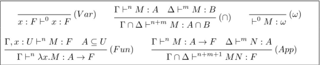
(V ar) x : F `0x : F Γ `n M : A ∆ `mM : B (∩) Γ ∩ ∆ `n+mM : A ∩ B (ω) `0M : ω Γ, x : U `nM : F A ⊆ U (F un) Γ `n λx.M : A → F Γ `n M : A → F ∆ `mN : A (App) Γ ∩ ∆ `n+m+1 M N : F
Figure 2.3: Typing rules
8. Greatest context: Γ ⊆ (). 9. (Γ, x : U ) ⊆ Γ.
Proof. Straightforward.
2.3.3
Rules
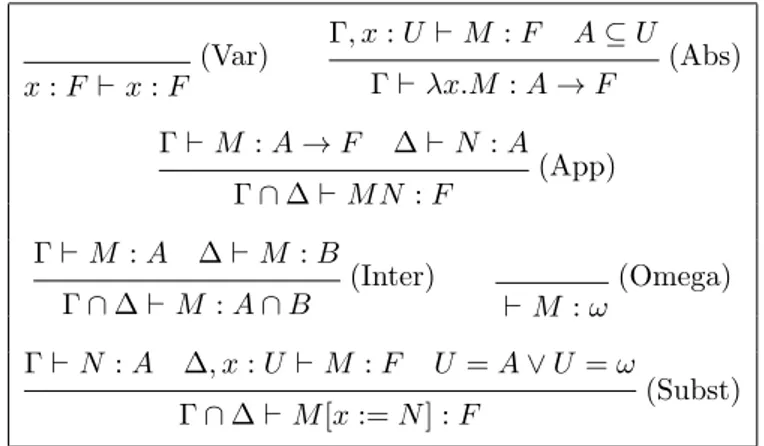
We now have all the elements to present the typing system: Definition 10 (Typing system).
Assume Γ is a context, M is a term, n is an integer, and U is a U -type. The judgement Γ `nM : U is inductively defined by the rules given in Figure 2.3.
We write Γ ` M : U if there exists n such that Γ `n M : U .
Some remarks:
• In Γ `n M : U , n is the number of uses of the rule (App) and it is the trivial
measure on typing trees that we use.
• The rule (ω) is a device to simplify some definitions, proofs and properties: it is independent from the other rules and this chapter could have been written without it (only with more cases in statements and proofs). In particular, ` M : ω gives no information about M and, for example, Theorem2uses A instead of U .
• Condition A ⊆ U in rule (F un) is called subsumption and is used to make Subject Reduction (Theorem1) hold when the reduction is under a λ: After a subject reduction, U can turn into a different U0 without changing A. • Another advantage in having the type ω for the presentation of the typing
system: Without the notation U or V , we would have to duplicate the ab-straction rule that types λx.M (one case where x ∈ fv(M ) and one case where x /∈ fv(M )). That would make two rules instead of one.
• Like the other judgements defined with induction rules, when we write “By induction on Γ ` M : U ”, means “By induction on the derivation proving Γ ` M : U ”.
Lemma 5 (Basic properties of typing).
1. Γ `n M : U ∩ V if and only if there exist Γ
1, Γ2, n1 and n2 such that Γ =
Γ1∩ Γ2, n = n1+ n2, Γ1`n1M : U and Γ2`n2M : V .
2. If Γ `n M : U and U ≈ V , then there exists ∆ such that Γ ≈ ∆ and
∆ `n M : V .
3. If Γ `nM : U and U ⊆ V , then there exist ∆ and m such that Γ ⊆ ∆, m ≤ n and ∆ `mM : V .
5. If Γ ` M : U , then Dom(Γ) ⊆ fv(M ). Proof. 1. Straightforward. 2. By induction on U ≈ V . 3. Corollary of 1 and 2. 4. By induction on Γ ` M : A. 5. Corollary of 4.
2.4
Soundness
As usual for the proof of Subject Reduction, we first prove a substitution lemma: Lemma 6 (Substitution lemma).
If Γ, x : U `n M : A and ∆ `mN : U , then there exists Γ0 such that Γ0≈ Γ ∩ ∆
and Γ0`n+mM {x := N } : A.
Proof. By induction on Γ, x : U ` M : A. The measure of the final typing tree is n + m because, by the fact that the intersection types are non-idempotent, this proof does not do any duplications of the rule (App).
More precisely: • For
x : F `0x : F with Γ = (), n = 0, M = x, U = F and A = F : We
have x{x := N } = N . By hypothesis, ∆ `m N : U . Therefore, ∆ `m
M {x := N } : F with n + m = m and Γ ∩ ∆ = () ∩ ∆ = ∆.
• For y : F `0y : F with y 6= x, Γ = (y : F ), n = 0, M = y, U = ω, and
A = F : By hypothesis, ∆ `m N : ω. Hence, ∆ = () and m = 0. We have
y{x := N } = y. Therefore, y : F `0 M {x := N } : F with n + m = 0 and Γ ∩ ∆ = (y : F ) ∩ () = (y : F ). • ForΓ1, x : U1` n1 M : A 1 Γ2, x : U2`n2M : A2 Γ1∩ Γ2, x : U1∩ U2`n1+n2 M : A1∩ A2 with Γ = Γ1∩ Γ2, n = n1+ n2, U = U1∩ U2 and A = A1∩ A2: By hypothesis, ∆ `m N : U1∩ U2. By
Lemma5.1, there exist ∆1, ∆2, m1and m2such that ∆ = ∆1∩∆2, m = m1+
m2, ∆1`m1N : U1and ∆2`m2 N : U2. By induction hypothesis, there exist
Γ01 and Γ02 such that Γ01 ≈ Γ1∩ ∆1, Γ02 ≈ Γ2∩ ∆2, Γ01 `
n1+m1 M {x := N } : A1 and Γ02 `n2+m2 M {x := N } : A2. Therefore, Γ01∩ Γ02 `n1+m1+n2+m2 M {x := N } : A1∩ A2 with Γ01∩ Γ02≈ (Γ1∩ ∆1) ∩ (Γ2∩ ∆2) ≈ (Γ1∩ Γ2) ∩ (∆1∩ ∆2) = Γ ∩ ∆ and n1+ m1+ n2+ m2= n + m. • For Γ, x : U, y : V ` n M 1: F B ⊆ V Γ, x : U `nλy.M1: B → F with M = λy.M1, x 6= y, y /∈ fv(N )
and A = B → F . We have (λy.M1){x := N } = λy.M1{x := N }. By
induction hypothesis, there exists Γ0such that Γ0 ≈ (Γ, y : V )∩∆ and Γ0`n+m
M1{y := N } : F . By Lemma5.5, Dom(∆) ⊆ fv(N ). Therefore, y /∈ Dom(∆)
and (Γ, y : V ) ∩ ∆ = (Γ ∩ ∆, y : V ). There exist a unique Γ00 and a unique V0 such that (Γ00, y : V0) = Γ0. Therefore, Γ00 ≈ Γ ∩ ∆ and V ≈ V0. Hence,
B ⊆ V0. Therefore, Γ00`n+mλy.M 1{x := N } : B → F . • ForΓ1, x : U1` n1 M 1: B → F Γ2, x : U2`n2 M2: B Γ1∩ Γ2, x : U1∩ U2`n1+n2+1M1M2: F with Γ = Γ1∩ Γ2, n = n1+ n2+ 1, U = U1∩ U2, M = M1M2 and A = F : We have (M1M2){x :=
N } = M1{x := N }M2{x := N }. By hypothesis, ∆ `m N : U1∩ U2.
By Lemma 5.1, there exist ∆1, ∆2, m1 and m2 such that ∆ = ∆1 ∩ ∆2,
m = m1+ m2, ∆1 `m1 N : U1 and ∆2 `m2 N : U2. By induction
hy-pothesis, there exist Γ01 and Γ02 such that Γ01 ≈ Γ1 ∩ ∆1, Γ02 ≈ Γ2∩ ∆2,
Γ01 `n1+m1 M1{x := N } : B → F and Γ02`n2+m2 M2{x := N } : B.
There-fore, Γ01∩ Γ02 `n1+m1+n2+m2+1 M1M2 : F with Γ01∩ Γ02≈ (Γ1∩ ∆1) ∩ (Γ2∩
∆2) ≈ (Γ1∩ Γ2) ∩ (∆1∩ ∆2) = Γ ∩ ∆ and n1+ m1+ n2+ m2+ 1 = n + m.
Theorem 1 (Subject Reduction).
If Γ `n M : A and M →
β M
0, then there exist Γ0 and n0 such that Γ ⊆ Γ0,
n > n0 and Γ0 `n0 M0: A.
Proof. First by induction on M →βM0, then by induction on A.
In particular, for the base case of the β reduction ( (λx.M 1)M 2 →β M1{x :=
M2}), we use Lemma6.
For the case λx.M1→βλx.M10 with M1→βM10, we use the fact that in the rule
(F un), there can be a subsumption. Therefore, the change of the type of x can be caught by the rule (App).
More precisely:
• If A is of the form A1∩ A2: Then, there exist Γ1, Γ2, n1 and n2 such that
Γ = Γ1∩ Γ2, n = n1+ n2, Γ1`n1 M : A1 and Γ2`n2 M : A2. By induction
hypothesis on (M →β M0, A1) and (M →β M 0, A
2), there exist Γ01, Γ02, n01
and n02 such that Γ1 ⊆ Γ01, Γ2 ⊆ Γ02, n1 > n01, n2 > n02, Γ01 `n
0 1 M0 : A1 and Γ02`n02M0: A 2. Therefore, Γ01∩ Γ02`n 0 1+n 0 2 M0: A1∩ A2with Γ = Γ1∩ Γ2⊆ Γ01∩ Γ0 2and n = n1+ n2> n01+ n02. • For (λx.M
1)M2→βM1{x := M2} with M = (λx.M1)M2 and A is of the
form F :
Therefore, there exist Γ1, Γ2, n1, n2, B such that Γ = Γ1∩Γ2, n = n1+ n2+ 1,
Γ1 `n1 λx.M1 : B → F and Γ2 `n2 M2 : B: Then, there exists U such that
B ⊆ U and Γ1, x : U `n1 M1 : F . By Lemma 5.3, there exist Γ02 and n02
such that Γ2 ⊆ Γ02, n2 ≥ n02 and Γ02 `n
0
2 M2 : U . By Lemma 6, there
exists Γ0 such that Γ0 ≈ Γ1 ∩ Γ02 and Γ0 `n1+n
0 2 M1{x := M2} : F with Γ = Γ1∩ Γ2⊆ Γ1∩ Γ02≈ Γ0 and n = n1+ n2+ 1 > n1+ n2≥ n1+ n02. • For M1→βM 0 1 λx.M1→βλx.M 0 1
with M = λx.M1and A is of the form F : There exist
B, G and U such that F = B → G, B ⊆ U and Γ, x : U `n M1 : G. By
induction hypothesis, there exists Γ01and n0 such that (Γ, x : U ) ⊆ Γ01, n > n0
and Γ0 1 `n
0
M0
1 : G. There exist a unique Γ0 and a unique U0 such that
Γ0
1= (Γ0, x : U0). Therefore, Γ ⊆ Γ0 and U ⊆ U0. Hence, B ⊆ U0. Therefore
Γ0`n0 λx.M0 1: B → G. • For M1→βM 0 1 M1M2→βM10M2
with M = M1M2and A is of the form F : There exist
Γ1, Γ2, n1, n2and B such that Γ = Γ1∩Γ2, n = n1+n2+1, Γ1`n1 M1: B → F
and Γ2`n2 M2: B. By induction hypothesis, there exist Γ01 and n01 such that
Γ1 ⊆ Γ01, n1 > n01 and Γ01 ` n0 1 M0 1 : B → F . Therefore, Γ01∩ Γ2 `n 0 1+n2+1 M10M2: F with Γ = Γ1∩ Γ2⊆ Γ01∩ Γ2 and n = n1+ n2+ 1 > n01+ n2+ 1. • For M2→βM 0 2 M1M2→βM1M20
with M = M1M2and A is of the form F : There exist
and Γ2`n2 M2: B. By induction hypothesis, there exist Γ02 and n02 such that Γ2⊆ Γ02, n2> n02and Γ02` n0 2 M0 2: B. Therefore, Γ1∩ Γ02` n1+n02+1M1M0 2: F with Γ = Γ1∩ Γ2⊆ Γ1∩ Γ02and n = n1+ n2+ 1 > n1+ n02+ 1.
In Theorem1, we have n > n0because, by the fact that types are non-idempotent, we do not do any duplications in the proof of Subject Reduction. Therefore, by Subject Reduction, for each β-reduction, the measure of the typing tree strictly decreases and then, we have Soundness as a corollary.
Theorem 2 (Soundness). If Γ `nM : A, then M ∈ SN
≤n.
Proof. Corollary of Theorem 1: We prove by induction on n that if Γ `n M : A
then M ∈ SN≤n.
Let M0 be a term such that M →β M0. By Theorem 1, there exist Γ0 and n0 such that n0< n and Γ0`n0
M0: A. By induction hypothesis, M0∈ SN≤n0. Hence,
M0∈ SN≤n−1 because n0≤ n − 1.
Therefore, M ∈ SN≤n.
Theorem 2 gives more information than a usual soundness theorem: If a term is typable, the term is not only strongly normalising, but the measure on a typing tree is a bound on the size longest β-reduction sequences from this term to its normal form. One of the reasons we have just a bound is that the measure of the typing tree can decrease more than 1. This is usually what happens when the β-reduction erases a sub-term. Having a better result than just a bound is discussed in Chapters3and4.
2.5
Semantics and applications
In this section we show how to use non-idempotent intersection types to simplify the methodology of [CS07], which we briefly review here:
The goal is to produce modular proofs of strong normalisation for various source typing systems. The problem is reduced to the strong normalisation of a unique tar-get system of intersection types, chosen once and for all. This is done by interpreting each term t as the set JtK of the intersection types that can be assigned to t in the target system. Two facts then remain to be proved:
1. if t can be typed in the source system, thenJtK is not empty 2. the target system is strongly normalising
The first point is the only part that is specific to the source typing system: it amounts to turning the interpretation of terms into a filter model of the source typ-ing system. The second point depends on the chosen target system: as [CS07] uses a system of idempotent intersection types (extending the simply-typed λ-calculus), their proof involves the usual reducibility technique [Gir72,Tai75]. But this is some-what redundant with point 1 which uses similar techniques to prove the correctness of the filter model with respect to the source system.
In this chapter we propose to use non-idempotent intersection types for the target system, so that point 2 can be proved with simpler techniques than in [CS07] while point 1 is not impacted by the move.
2.5.1
Denotational semantics
The following filter constructions only involve the syntax of types and are indepen-dent from the chosen target system.
Definition 11 (Values).
A value v is a set of U -types such that: • ω ∈ v.
• If U ∈ v and U ⊆ V , then V ∈ v. • If U ∈ v and V ∈ v, then U ∩ V ∈ v. We write D the set of values.
While our intersection types differ from those in [CS07] (in that idempotency is dropped), the stability of a filter under type intersections makes it validate idem-potency (it contains A if and only if it contains A ∩ A, etc). This makes our filters very similar to those in [CS07], so we can plug-in the rest of the methodology with minimal change.
Definition 12 (Examples of values). 1. Let ⊥ := {ω}
2. Let >, the set of all U -types.
3. Assume α is a set of F -types. Then < α > is the set of U -types defined with the following rules:
F ∈ α
F ∈< α > ω ∈< α >
A ∈< α > B ∈< α > A ∩ B ∈< α > 4. Assume u, v ∈D. Let uv := < {F | ∃A ∈ v, (A → F ) ∈ u} >.
Lemma 7 (Properties of values). Assume u, v ∈D.
1. If for all F ∈ u we have F ∈ v, then u ⊆ v.
2. If for all F , F ∈ u if and only if F ∈ v, then u = v.
3. ⊥ is the smallest element ofD and > is the biggest element of D. 4. If U ∈ v and U ≈ V , then V ∈ v.
5. < α > is the smallest element v of D such that α ⊆ v. 6. F ∈< α > if and only if F ∈ α.
7. uv ∈D and F ∈ uv if and only if there exists A such that (A → F ) ∈ u and A ∈ v.
8. We have u⊥ = ⊥ = ⊥u. 9. If v 6= ⊥, then >v = >.
Proof.
1. We prove by induction on U , that for all U ∈ u, we have U ∈ v: • For ω: By Definition11, we have ω ∈ v.
• For F : By hypothesis, we have F ∈ v.
• For A ∩ B: We have A ∩ B ⊆ A and A ∩ B ⊆ B. By Definition11, we have A ∈ u and B ∈ u. By induction hypothesis, we have A ∈ v and B ∈ v. By Definition11, we have A ∩ B ∈ v.
2. Corollary of 1.
3. First, we prove that ⊥ ∈D: • We have ω ∈ ⊥.
• Assume U ∈ ⊥ and U ⊆ V . Therefore, U = ω and ω ⊆ V . We also have V ⊆ ω. Hence, V ≈ ω. Therefore, V = ω and V ∈ ⊥.
• Assume U ∈ ⊥ and V ∈ ⊥. Therefore, U = ω and V = ω. Hence, U ∩ V = ω ∩ ω = ω ∈ ⊥.
Therefore, ⊥ ∈D.
Assume v ∈ D and U ∈ ⊥. Then, U = ω and U ∈ v. Hence, ⊥ ⊆ v.
Therefore, ⊥ is the smallest element ofD.
It is straightforward to prove that > is the biggest element ofD.
4. Assume U ∈ v and U ≈ V . Then, U ⊆ V . Therefore, by Definition11, V ∈ v. 5. To prove that < α >∈D we first need the following:
• We can notice that U ∩V ∈< α > if and only if U ∈< α > and V ∈< α >. • We can prove by induction U ≈ V , that if U ∈< α > and U ≈ V then
V ∈< α >.
Therefore, we can prove that < α >∈D: • We have ω ∈< α >.
• Assume U ∈< α > and U ⊆ V . Hence, there exists U0 such that
U ≈ V ∩ U0. Therefore, V ∩ U0 ∈< α >. Hence, V ∈< α >. • If U ∈< α > and V ∈< α >, then U ∩ V ∈< α >.
Therefore, < α >∈D and by definition we have α ⊆< α >.
Assume v ∈ D such that α ⊆ v. We can prove by induction on U ∈< α > that for all U ∈< α >, we have U ∈ v. Hence, < α >⊆ v.
Therefore, < α > is the smallest element v ofD such that α ⊆ v. 6. Straightforward.
7. The fact that uv ∈D is a corollary of 5. The rest is a corollary of 6. 8. By 3, we have ⊥ ⊆ u⊥ and ⊥ ⊆ ⊥u.
• Assume F ∈ u⊥. Then, by 7, there exists A such that (A → F ) ∈ u and A ∈ ⊥. Contradiction. Therefore, F ∈ ⊥.
By 1, u⊥ ⊆ ⊥.
• By a similar proof, ⊥u ⊆ ⊥. Therefore, u⊥ = ⊥u = ⊥. 9. By 3, we have >v ⊆ >.
Assume F ∈ >. By the fact that v 6= ⊥, there exists A ∈ v. Therefore, (A → F ) ∈ > and F ∈ >v.
By 1, we have > ⊆ >v. Then, we can conclude.
Definition 13 (Environements).
An environment ρ is a total map from the set of variables toD. Assume Γ is a context, then we write Γ ∈ ρ if and only if:
∀x, Γ(x) ∈ ρ(x) The environment (ρ, x v) is defined as follow:
(ρ, x v)(x) := v
(ρ, x v)(y) := ρ(y) (x 6= y)
Lemma 8 (Properties of environments).
2. If Γ ∈ (ρ, x v), then there exist Γ0 and U such that Γ = (Γ0, x : U ), Γ0 ∈ ρ and U ∈ v.
3. We have () ∈ ρ.
4. If Γ ∈ ρ and Γ ⊆ ∆, then ∆ ∈ ρ. 5. If Γ ∈ ρ and ∆ ∈ ρ, then Γ ∩ ∆ ∈ ρ.
Proof. By the fact that Γ ∈ ρ is defined point-wise.
Definition 14 (Semantics of a term).
Assume M is a term and ρ an environment. Let JM Kρ:= {U | ∃Γ ∈ ρ, Γ ` M : U }.
Lemma 9 (Properties of the semantics of a term). 1. We haveJM Kρ ∈D.
2. IfJM Kρ6= ⊥, then M is strongly normalising.
3. We haveJxKρ= ρ(x). 4. We haveJM N Kρ=JM KρJN Kρ. 5. We haveJλx.M Kρv ⊆JM K(ρ,x v). 6. If x ∈ fv(M ) or v 6= ⊥, then Jλx.M Kρv =JM K(ρ,x v). 7. If M →βM0, thenJM Kρ⊆JM 0 Kρ. Proof. 1. We prove thatJM Kρ∈D:
• We have ` M : ω and () ∈ ρ (by Lemma8.3). Therefore, ω ∈JM Kρ.
• Assume U ∈ JM Kρ and U ⊆ V . Then, there exists Γ ∈ ρ such that
Γ ` M : U . Therefore, there exists Γ0 such that Γ ⊆ Γ0 and Γ0` M : V . By Lemma8.4, we have Γ0 ∈ ρ. Hence, V ∈JM Kρ.
• Assume U ∈JM Kρ and V ∈JM Kρ. Then, there exist Γ, ∆ ∈ ρ such that Γ ` M : U and ∆ ` M : V . Therefore, Γ ∩ ∆ ` M : U ∩ V and by Lemma8.5, Γ ∩ ∆ ∈ ρ. Hence, U ∩ V ∈JM Kρ.
Therefore,JM Kρ∈D.
2. Assume JM Kρ 6= ⊥. Then, there exists A ∈ JM Kρ. Therefore, there exists Γ ∈ ρ such that Γ ` M : A. By Theorem2, M is strongly normalising. 3.
• Assume F ∈ JxKρ. Then, there exists Γ ∈ ρ such that Γ ` x : F . Therefore, Γ = (x : F ) and F = Γ(x). We also have Γ(x) ∈ ρ(x). Hence, F ∈ ρ(x).
• Assume F ∈ ρ(x). Then, (x : F ) ∈ ρ and x : F ` x : F . Therefore, F ∈JxKρ.
By Lemma7.2,JxKρ= ρ(x).
4.
• Assume F ∈JM N Kρ. Then, there exists Γ ∈ ρ such that Γ ` M N : F .
Therefore, there exist Γ1, Γ2 and A such that Γ = Γ1∩ Γ2, Γ1 ` M :
A → F and Γ2 ` N : A. We have Γ ⊆ Γ1 and Γ ⊆ Γ2. By Lemma 8.4,
Γ1 ∈ ρ and Γ2 ∈ ρ. Hence, (A → F ) ∈ JM Kρ and A ∈ JN Kρ. By Lemma7.7, F ∈JM KρJN Kρ.
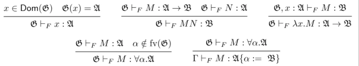
x ∈ Dom(G) G(x) = A G`F x : A G`F M : A → B G`F N : A G`F M N : B G, x : A `F M : B G`F λx.M : A → B G`F M : A α /∈ fv(G) G`F M : ∀α.A G`F M : ∀α.A Γ `F M : A{α := B}
Figure 2.4: Typing rules of System F
• Assume F ∈JM KρJN Kρ. By Lemma 7.7, there exists A such that (A → F ) ∈ JM Kρ and A ∈ JN Kρ. Then, there exist Γ1, Γ2 ∈ ρ such that Γ1 ` M : A → F and Γ2 ` N : A. Therefore, Γ1∩ Γ2 ` M N : F . By
Lemma8.5, Γ1∩ Γ2∈ ρ. Hence, F ∈JM N Kρ. By Lemma7.2,JM N Kρ=JM KρJN Kρ.
5. Assume F ∈Jλx.M Kρv. By Lemma 8.5, there exists A such that (A → F ) ∈
Jλx.M Kρ and A ∈ v. Then, there exists Γ ∈ ρ such that Γ ` λx.M : A → F . Hence, there exist U such that A ⊆ U and Γ, x : U ` M : F . Therefore, U ∈ v. By Lemma8.1, (Γ, x : U ) ∈ (ρ, x v). Hence, F ∈JM K(ρ,x v). By Lemma7.1,Jλx.M Kρv ⊆JM K(ρ,x v).
6. By 5, we haveJλx.M Kρv ⊆JM K(ρ,x v).
Assume F ∈JM K(ρ,x v). Then, there exists Γ ∈ (ρ, x v) such that Γ ` M : F . By Lemma7.2, there exist Γ1 ∈ ρ and U ∈ v such that Γ = (Γ1, x : U ).
Therefore, Γ1, x : U ` M : F . By hypothesis, we are in one of the following
cases:
• We have x ∈ fv(M ): Therefore, U is of the form A. • We have v 6= ⊥ and U is of the form A.
• We have v 6= ⊥ and U = ω: Then, there exists A ∈ v and we have A ⊆ ω. In all cases, there exists A ∈ v such that A ⊆ U . Hence, Γ1` λx.M : A → F .
Therefore, (A → F ) ∈Jλx.M Kρ. By Lemma7.7, F ∈Jλx.M Kρv. By Lemma7.1,JM K(ρ,x v)⊆Jλx.M Kρv.
Then, we can conclude.
7. Assume F ∈ JM Kρ. Then, there exists Γ ∈ ρ such that Γ ` M : F . By
Theorem1, there exists Γ0such that Γ ⊆ Γ0 and Γ0` M0 : F . By Lemma8.4,
Γ0∈ ρ. Therefore, F ∈JM0 Kρ. By Lemma7.1,JM Kρ⊆JM 0 Kρ.
2.5.2
Example: System F
Definition 15 (System F).Types of System F are defined with the following grammar: A, B, C ::= α | A → B | ∀α.A
where α ranges over an infinite set of type variables. Free variables and substitution is defined the usual way.
A context G in System is a partial map from type variables to types of System F.
The typing judgement G `F M : A is defined with the rules of Figure 2.4.
Definition 16 (Model of System F).
• > ∈ X. • ⊥ /∈ X.
Assume X, Y ∈ TP(D).
Let X → Y := {u ∈D | ∀v ∈ X, uv ∈ Y }.
Lemma 10 (Examples of elements of TP(D)).
1. We have {>} ∈ TP(D).
2. Assume (Xi)i∈I a non-empty family of TP(D). Then, Ti∈IXi∈ TP(D).
3. Assume X, Y ∈ TP(D). Then X → Y ∈ TP(D).
Proof.
1. Straightforward. 2. Straightforward. 3.
• Assume v ∈ X. Then, by Definition16, we have v 6= ⊥. By Lemma7.9, >v = >. By Definition16, we have > ∈ Y . Therefore, > ∈ X → Y . • Assume ⊥ ∈ X → Y . We have > ∈ X. Therefore, we have ⊥> ∈ Y . By
Lemma7.8, ⊥> = ⊥. Therefore, ⊥ ∈ Y . Contradiction. Hence, ⊥ /∈ X → Y .
Therefore, X → Y ∈ TP(D).
Definition 17 (Interpretation of System F in the TP(D)).
Assume σ a total map from type variables α to TP(D) ( type environment). We define [A]σ∈ TP(D) by induction on A as follows:
[α]σ := σ(α)
[A → B]σ := [A]σ→ [B]σ
[∀α.A]σ := TX∈TP(D)[A](σ,α X)
We define [G]σ as the set of environment ρ such that:
∀x ∈ Dom(G), ρ(x) ∈ [G(x)]σ
Theorem 3 (Soundness of the model). Assume G `F M : A.
Then, for all σ type environment we have: ∀ρ ∈ [G]σ,JM Kρ∈ [A]σ Proof. By induction on G `F M : A.
• Forx ∈ Dom(G) G(x) = A
G`F x : A
with M = x: Therefore,JxKρ= ρ(x) (by Lemma9.3).
And we have ρ(x) ∈ [G(x)]σ = [A]σ.
• For G`F M1: B → A G`F M2: B G`F M1M2: A
with M = M1M2: By Lemma 9.4,
JM1M2Kρ = JM1KρJM2Kρ. By induction hypothesis, JM1Kρ ∈ [B → A]σ = [B]σ→ [A]σ andJM2Kρ∈ [B]σ. Therefore,JM1KσJM2Kσ∈ [A]σ.
• For G, x : A1`F M1: A2 G`F λx.M1: A1→ A2
with M = λx.M1 and A = A1→ A2:
Assume v ∈ [A1]σ. Then, v 6= ⊥. By Lemma9.6,Jλx.M1Kρv =JM1K(ρ,x v). We also have (ρ, x v) ∈ [G, x : A1]σ. By induction hypothesis,JM1K(ρ,x v)∈ [A2]σ. Therefore,Jλx.M1Kρv ∈ [A2]σ.
• ForG`F M : A1 α /∈ fv(G) G`F M : ∀α.A1
with A = ∀α.A1:
Assume X ∈ TP(D). By the fact that α /∈ fv(G), we have [G](σ,α X)= [G]σ.
Therefore, ρ ∈ [G](σ,α X). By induction hypothesis,JM Kρ∈ [A1](σ,α X). Hence,JM Kρ ∈TX∈TP(D)[A1](σ,α X)= [∀α.A1]σ= [A]σ.
• For G`F M : ∀α.A1
G`F M : A1{α := A2}
with A = A1{α := A2}:
By induction hypothesis,JM Kρ ∈ [∀α.A1]σ =TX∈TP(D)[A1](σ,α X). In
par-ticular, JM Kρ ∈ [A1](σ,α [A2]σ). We can prove by induction on A1 that
[A1{α := A2}]σ= [A1](σ,α [A2]σ). Therefore,JM Kρ∈ [A]σ.
Theorem 4 (Strong normalisation of System F). If G `F M : A, then M is strongly normalising.
Proof.
Let σ defined by: ∀α, σ(α) := {>}.
Let ρ defined by: ∀x, ρ(x) := >. Therefore, ρ ∈ [G]σ.
By Theorem3, we haveJM Kρ∈ [A]σ. Therefore,JM Kρ6= ⊥. By Lemma9.2, M is strongly normalising.
2.6
Completeness
The goal of this section is to prove that if a term is strongly normalising, then it is typable. We use the same method usually done to prove this result with idempotent intersection type:
• We exhibit a β-reduction sequence from M to its normal form M0.
• We type M0.
• To get a typing of M we backtrack from M0: For each β-step M
1→βM2, we
get a typing of M1 from a typing of M2.
What we do in each β-step is called Subject Expansion (Theorem5). Unfortunately, Subject Expansion does not work for every reduction M →β M0. In particular, it
does not hold when M /∈ SN and M0 ∈ SN (by Theorem 2). Here are a few
examples bellow:
• Case where the argument of the β-redex is not strongly normalising and is erased:
(λx.y)((λz.zz)(λz.zz)) →β y • More subtle case:
(λw.(λx.y)(ww))(λz.zz) →β(λw.y)(λz.zz)
Here, the erased term ww is strongly normalising but w, one of its free variable is caught by the abstraction λw.
Therefore, we need a restricted reduction relation such that: • It can reach the normal form.
• It satisfies Subject Expansion. Therefore, it preserves strong normalisation both ways.
The restricted reduction relation that we give here is not the smallest one that satisfies those properties. On the contrary, we try to define the biggest one that satisfies them. This gives us a better understanding about operational semantics and intersection types and it gives more weight to some theorems such as Theorem2.6
(which states that this strategy is perpetual ).
First, we have to understand why we cannot directly adapt the proof of Subject Reduction to prove Subject Expansion:
• For M1→β M2: When an argument N of a β-redex is erased, to type M1, we
need to type N and we have no information about how to type N from the typing of M2. (first example)
• When a term is erased, the type of a context changes after Subject Expansion (it gets bigger). When dealing with the (App) rule, we are in a similar situ-ation that we were in Subject Reduction. To avoid this problem, in Subject Reduction, we can have a subsumption but here the subsumption is on the wrong side.
Therefore, when doing an erasure, we have to make sure that the variables of the erased term are not caught by a lambda like in the second example. Hence, it seems logic to keep information about the set of variables E of an erased terms when defining the strategy.
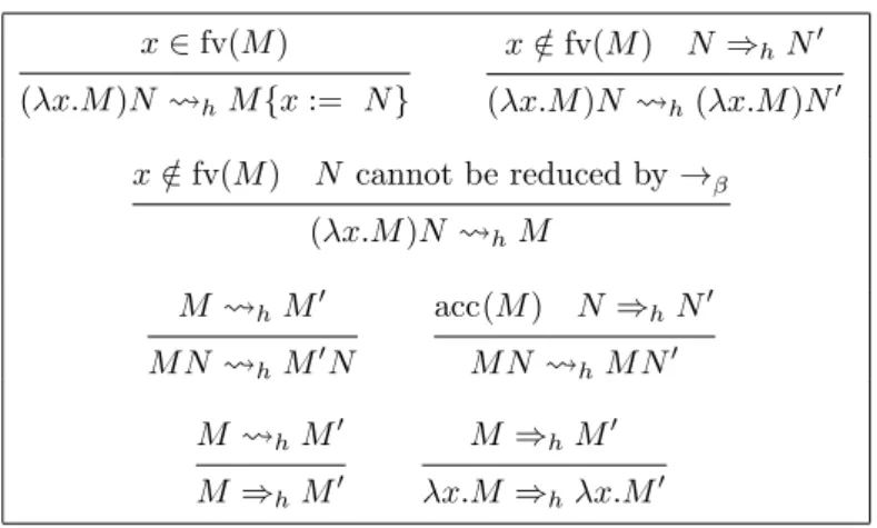
We actually introduce, two restricted reduction relations that are mutally de-fined: E and ⇒E. The second one is more general than the first. This definition
uses an “accumulator property” denoted accx(M ) (accx(M ) if and only if M is of
the form xM1. . . Mn; we also say that x is the head variable of M ). The rules
are given in Figure 2.5 and are purely syntactic. However, their motivation and meaning is that:
• If M cannot be reduced by →β, then M is typable.
• If accx(M ) and M is typable, then we can give M any type by just changing
the type of x.
• If M E M0 and M0 is typable with a type A, then M has type A, just by
changing the types of each x in E.
• If M ⇒E M0and M0 is typable with a type A, then M is typable with a type
B (which can be different from A), just by changing the types of each x in E. In more simple and common perpetual strategies (such as the one defined in Chap-ter 4) we do not need E.
More formally:
Definition 18 (Accumulators).
Assume M is a term and x a variable. Then, accx(M ) is defined with the
following rules:
accx(x)
accx(M )
accx(M N )
We write acc(M ) if there exists x such that accx(M ).
Definition 19 (Special reductions).
Assume M and M0 are terms and E is a finite set of variables. The reductions M EM0 and M ⇒EM0 are defined with the rules of Figure2.5.
Lemma 11 (Execution of a λ-term).
1. If M cannot be reduced by →β, then we are in one of the following cases: • M is of the form λx.M1.
x ∈ fv(M ) (λx.M )N ∅M {x := N } x /∈ fv(M ) N ⇒E N0 (λx.M )N E (λx.M )N0 x /∈ fv(N ) N cannot be reduced by →β (λx.M )N fv(N )M M EM0 M N EM0N N E N0 M N E M N0 M EM0 x /∈ E λx.M Eλx.M0 M EM0 M ⇒EM0 M ⇒E M0 λx.M ⇒E−{x}λx.M0 accx(M ) N ⇒EN0 M N E∪{x}M N0
Figure 2.5: Rules of E and ⇒E
2. If M can be reduced by →β, then there exists E and M0 such that M ⇒EM0.
Moreover, if M is not of the form λx.M , then there exist E and M0 such that M EM0.
3. If M EM0, then M ⇒EM0.
4. If M ⇒EM0 then M →βM0.
Proof.
1. By induction on M - see e.g. [B¨oh68].
2. By induction on M : We are in one of the following cases:
• M is of the form x: Then, M cannot be reduced by →β. Contradiction. • M is of the form λx.M1: Then, M1can be reduced by →β. By induction
hypothesis, there exist E and M10 such that M1 ⇒E M10. Therefore,
M ⇒Eλx.M10.
• M is of the form (λx.M1)M2and x ∈ fv(M1): Therefore, M ∅M1{x :=
M2}.
• M is of the form (λx.M1)M2, x /∈ fv(M1) and M2can be reduced by →β:
By induction hypothesis, there exist E and M20 such that M2 ⇒E M20.
Therefore, M E(λx.M1)M20.
• M is of the form (λx.M1)M2, x /∈ fv(M1) and M2cannot be reduced by
→β: Therefore, M fv(M2)M1.
• M is of the form M1M2, M1 is not of the form λx.M3 and M1 can be
reduced by →β: By induction hypothesis, there exist E and M10 such that M1 E M10. Therefore, M EM10M2.
• M is of the form M1M2, M1 is not of the form λx.M3 and M1 cannot
be reduced by →β: By 1, there exists x such that accx(M ).
If M2 cannot be reduced by →β, then M cannot be reduced by →β.
Contradiction. Therefore, M2 can be reduced by →β.
By induction hypothesis, there exist E and M20 such that M2 ⇒E M20.
Therefore, M E∪{x}M1M20.
In all cases, if M EM0, then M ⇒EM0.
3. Trivial.
4. We prove the following by induction on M E M0 and by induction on