Structurally Parameterized Tight Bounds and Approximation for Generalizations of Independence and Domination

(1)

Préparée à l’Université Paris-Dauphine

Structurally Parameterized Tight Bounds and

Approximation for Generalizations of

Independence and Domination

Soutenue par

Ioannis KATSIKARELIS

Le 12/12/2019 École doctorale no₅₄₃

ED de Dauphine

Spécialité

Informatique

Composition du jury : Mathieu LIEDLOFF Maître de Conférences,

Université d’Orléans Rapporteur

Ignasi SAU VALLS

Chargé de Recherche CNRS,

LIRMM Montpellier Rapporteur

Bruno ESCOFFIER

Professeur,

Sorbonne Université Examinateur

Ioan TODINCA

Professeur,

Université d’Orleans Président du jury

Michail LAMPIS

Maître de Conférences,

Université Paris-Dauphine Codirecteur de thèse

Vangelis Th. PASCHOS

Professeur,

(2)

(3)

Acknowledgements

As an expression of my sincere gratitude towards (1) my supervisors Vangelis Th. Paschos and Michail Lampis; (2) the members of my jury Bruno Escoﬃer, Mathieu Liedloﬀ, Ignasi Sau Valls and Ioan Todinca; (3) my co-authors (and Sakura people) Rémy Belmonte, Tesshu Hanaka, Mehdi Khosravian Ghadikolaei, Eun Jung Kim, Valia Mitsou, Hirotaka Ono, Yota Otachi and Florian Sikora; (4) all of LAMSADE and anyone else who may have contributed to the making of the present thesis: merci beaucoup !

(4)

(5)

5 On the (Super-)Polynomial (In-)Approximability of d-Scattered Set 93 5.1 Super-polynomial time . . . 95 5.1.1 Inapproximability . . . 95 5.1.2 Approximation . . . 98 5.2 Polynomial Time . . . 100 5.2.1 Inapproximability . . . 100 5.2.2 Approximation . . . 104 5.2.3 Bipartite graphs . . . 106 6 Conclusion 109

7 Résumé des chapitres en français 113

(6)

(7)

1

Introduction

The aim of computational complexity theory is the categorization of mathematical prob-lems into classes according to the worst-case running-times of the algorithms that solve them. In the classical setting problems are considered tractable, that is, polynomial-time solvable, if there exists an algorithm whose running-time can be expressed as a polynomial function on the size n of the input. On the other hand, the intractable problems (com-monly NP-hard1_{) are those for which a polynomial-time algorithm is considered unlikely,}

based on the (widely believed) conjecture that P6=NP: if the 3-SAT problem does not ad-mit a deterministic polynomial-time algorithm, then a reduction from 3-SAT to another problem, i.e. a transformation from one problem’s instances to the other’s demonstrat-ing their equivalence in terms of computational complexity, would imply that the latter problem does not admit a polynomial-time algorithm as well.

Taking the above considerations one step further leads to the formulation of another (also widely believed) conjecture, the Exponential Time Hypothesis (ETH): it conjectures there is no subexponential algorithm for 3-SAT, i.e. no algorithm of running-time 2o(n)_·

nO(1). If this hypothesis is true, then P is not equal to NP and any algorithm for 3-SATwill require at least exponential time, in the worst case. A slightly more demanding (and not-so-widely believed) version, the Strong Exponential Time Hypothesis (SETH) has also been formulated and asserts that (general) SAT does not admit an algorithm of running-time (2 − ǫ)n_{· n}O(1) _{for any constant ǫ > 0.}

As with the assumption that P6=NP, the main importance of the ETH and SETH, however, lies not in whether these may actually be true or not: in a similar manner as in the classiﬁcation of problems into polynomial-time solvable or NP-hard, we can use the ETH and SETH as starting points in showing, via hardness reductions, the non-existence of any algorithm of some specific running-time below a certain threshold and in this way derive results that preclude the existence of such algorithms for a given problem (a lower bound). Combining results of this type with algorithms whose worst-case (or upper bounded) running-times exactly match these lower bounds, we can precisely identify the complexity of a given problem and justify the optimality of our approach. Naturally, any such statements we make will be subject to the above assumptions, meaning our results will imply the proposed algorithms are optimal, unless signiﬁcant progress is made in our understanding of the fundamental principles of computation.

1_{So as not to overload this preface with notation, all formal definitions of the technical terms we freely}

discuss here are postponed until Section 2.1, along with the related bibliographical references.

(8)

In this way, we can further classify problems according to their exact computational requirements, especially in the case of the SETH that offers a more precise source at the cost of a more ambitious (and therefore more likely to be incorrect) assumption. This re-finement importantly allows us to advance our understanding of the available options for tackling a provably demanding computational problem and can potentially lead to practi-cal improvements in applied settings, yet it is the possibility of precisely characterizing the underlying complexity features of mathematical problems that will be mostly of interest to us here. Having shown both an upper and a lower bound of matching complexity functions for a given problem (i.e. bounds that are tight), we can usually identify a uniformity in the mathematical structure of the two proofs that is not arbitrary, as in the optimality of a reduction that will produce instances (almost) explicitly constructed to hinder the efforts of the algorithm whose running-time exactly matches the reduction’s lower bound (and vice-versa). Results such as these can be seen as implying that an aspect of the problem’s essence has been undeniably identified, since their validity does not depend on the particular methods employed by their designer.

Parameterization and Approximation Being able to characterize the intractability of a problem according to a particular mode of computation does not mean we have exhausted all possibilities for addressing it. Regarding a problem as intractable if the required running-time of any algorithm for its exact solution is at least exponential in the size of the input can thus lead to other directions for advancing our comprehension of the intricate mechanisms that regulate complex combinatorial problems: parameterization and approximation. On one hand and in search of a ﬁner characterization of the necessary amount of computation needed for the exact and optimal resolution of a computational problem, we could allow the complexity functions to grow indeed exponentially, but not on the size n of the input (that must naturally be considered too large and impractical). Via parameterization we study the complexity of problems in terms of other parameters that specify their properties than simply the size of the input, parameters whose (bounded) size would not preclude practical computations of an exponential number. On the other hand, relaxing the requirement that the solutions returned by our algorithms are necessarily the best possible (being of measurable quality for optimization problems) and focusing on keeping the running-times polynomial on the size of the input, we enter the realm of approximation. Here, our solutions must be accompanied by mathematical guarantees of remaining above certain quality thresholds (a worst-case approximation ratio).

In parameterized complexity, similarly to the classiﬁcation of problems as NP-hard or polynomial-time solvable, a mathematical problem that is solved by an algorithm whose complexity can be expressed as a function of the form f(k) · nO(1)_{, where k is the}

cho-sen parameter and f is any computable function, belongs to the class of fixed-parameter tractable problems (FPT). Depending on the problem, the functions f may take on many forms, being exponential in the majority of cases. This implies that should the size of the parameter under consideration not be too large, for a given instance of a problem to be solved, then an FPT algorithm that solves it could be considered usable (perhaps even practical), while also providing important reﬁnements on the complexity landscape in general. Common parameters include the size of an optimal solution (the standard pa-rameterization), as well as a variety of structural measures that characterize the inherent structure of the input instance. Here, a problem is considered intractable if it can be shown (via parameterized reductions, also maintaining a close relationship between parameters)

(9)

to be as hard to solve as any problem that is complete for a level of the W-hierarchy of complexity classes (considered an analogue of NP-hardness), i.e. if it is unlikely to be FPT. The theory of approximation algorithms concerns itself with the complementary side of intractability: identifying the best possible worst-case bounds on the quality of a returned solution that can be obtained if the running-time is conﬁned to the polynomials in n. These bounds are commonly expressed as the ratio between the worst-case quality of a returned solution and that of an optimal solution for the same instance. On the ‘hardness’ side, it is possible to show (via approximation-preserving reductions) that there is no polynomial-time algorithm achieving a certain ratio for a given problem, under standard complexity assumptions, thus establishing its inapproximability. Common ratios in results of this type include inapproximability to speciﬁc constants, to any possible constant ratio, as well as a ratio that is a function of n. The allowed running-time for an approximation algorithm is commonly polynomial in n, yet it is possible to allow other functions (such as FPT running-times) in order to propose alternatives to exact computation, should a problem remain intractable beyond the polynomial-time boundary.

Returning once more to the ETH and SETH, we may observe that in conjunction with the reﬁned complexity analysis performed by the studies of parameterization it is possible to obtain improved lower bounds of increased precision on the required running-time of any algorithm for a given problem. Both hypotheses can be considered as assumptions on the complexity of q-SAT parameterized by the number of variables n and a param-eterized reduction to another problem in this case (i.e. where the size of the parameter is bounded by an appropriate function of n) would yield results on the non-existence of a subexponential (in the size of the parameter) algorithm for the problem in question. Thus parameterized problems can be further categorized in terms of the exact functions that determine their complexity with respect to the variety of possible parameters that partake in their intractability, leading to a much-improved understanding of the ﬁeld of computational complexity.

Covering and Packing problems: In this thesis we focus on the well-known

graph-theoretical problems (k, r)-Center and d-Scattered Set that generalize the concepts of vertex domination and independence over larger distances within the graph. In the Dominating Set problem we are looking for the smallest subset of vertices such that every other vertex is connected to at least one vertex in the subset. On the other hand, in Independent Set we require the largest subset such that no pair of vertices in the subset have an edge between them. Intuitively, a dominating set must cover the rest of the graph based on the combined adjacency of its vertices to those of the complement, while in an independent set we must be able to pack as many pairwise non-adjacent vertices as possible. Both problems exhibit ﬁrm intractability: they are NP-hard, their standard parameterizations W-hard and generally inapproximable in polynomial- as well as FPT-time. On the positive side, both problems turn out to be FPT when parameterized by the most widely-used structural parameters. This means that when the input graph is of restricted structure, both problems can be eﬃciently, as well as exactly solved.

The generalizations of these well-studied notions that we will be examining here are based on extending the central distance parameter in their deﬁnitions to unbounded values. In (k, r)-Center we are asked for the smallest set that covers the graph at distance r and in d-Scattered Set we must pack as many vertices as possible at distance d from each other. This means our perspective here must expand to consider the inﬂuence of

(10)

vertices taking part in the solution over larger areas within the graph, as the significance of adjacency lies now with paths instead of edges. As a preliminary remark, it turns out that reachability between vertices is too responsive a property to small shifts in their exact location, making the existence of collections of paths of non-trivial length crucially depend on the exact shape of local structures and therefore the behaviour of both problems will diverge (significantly) from their base cases when r, d are large. This effect is reflected in our results, since both problems become intractable even for graphs of significantly restricted structure, if the value of the distance parameter is not bounded in each case. Thus the above-mentioned algorithms are efficient only for small, fixed values (e.g. r = 1, d = 2), motivating our subsequent analysis.

Our Scope: We will consider the problems (k, r)-Center and d-Scattered Set,

pay-ing particular attention to how their complexity is aﬀected by the distance parameters and to the available options for their exact and/or eﬃcient computation. Since our problems are in fact generalizations of Dominating Set and Independent Set, our results can be seen to match (and sometimes even improve) the state-of-the-art for these problems.

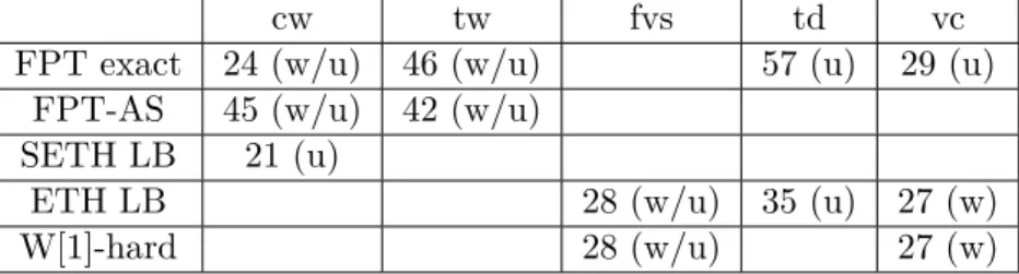
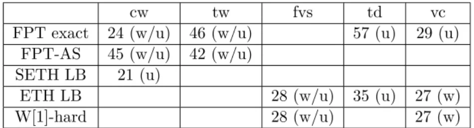
In the first part of the thesis we maintain a parameterized viewpoint: we examine the standard parameterization, as well as the most commonly used graph measures treewidth tw, clique-width cw, tree-depth td, vertex cover vc and feedback vertex set fvs. We offer hardness results that show there is no algorithm of running-time below certain bounds (subject to the ETH, SETH), produce essentially optimal algorithms of complexity that matches these lower bounds and further attempt to offer an alternative to exact compu-tation in significantly reduced running-time by way of approximation. In particular, for (k, r)-Center we show the following:

• A dynamic programming algorithm of running-time O∗_{((3r + 1)}cw_{), assuming a}

clique-width expression of width cw is provided along with the input, and a match-ing SETH-based lower bound that closes a complexity gap for Dominatmatch-ing Set parameterized by cw (for r = 1).

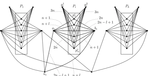
• W[1]-hardness and ETH-based lower bounds of no(vc+k) for edge-weighted graphs and no(fvs+k) _{for unweighted graphs. This shows the importance of bounding the}

value of r. Also for the unweighted case, we give an O∗₍₅vc_{)-time FPT algorithm}

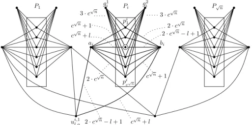
based on solving appropriate Set Cover sub-instances. • A tight ETH-based lower bound of O∗₍₂O(td)2

) for parameterization by td.

• Algorithms computing for any ǫ > 0, a (k, (1+ǫ)r)-center in time O∗_((tw/ǫ)O(tw)_{), or}

O∗((cw/ǫ)O(cw)), if a (k, r)-center exists in the graph, assuming a tree decomposition of width tw is provided along with the input.

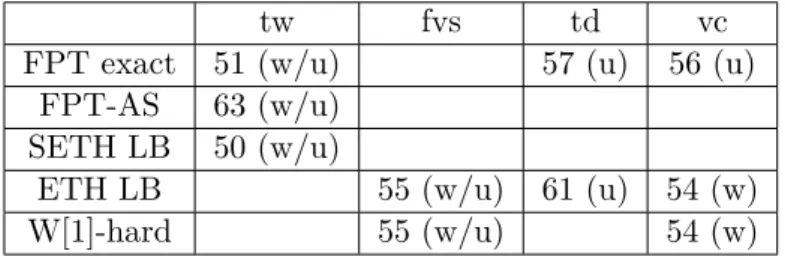
Then for d-Scattered Set and applying similar methods we show:

• A dynamic programming algorithm of running-time O∗_(dtw_{) and a matching lower}

bound based on the SETH, that generalize known results for Independent Set. • W[1]-hardness for parameterization by vc+k for edge-weighted graphs, as well as by

fvs + k for unweighted graphs, again showing the importance of bounding d. These are complemented by FPT-time algorithms for the unweighted case that use ideas related to Set Packing, of complexity O∗₍₃vc_{) for even d and O}∗₍₄vc_{) for odd d.}

(11)

• A tight ETH-based lower bound of O∗(2O(td)2) for parameterization by td, as above. • An algorithm computing, for any ǫ > 0, a d/(1+ǫ)-scattered set in time O∗_((tw/ǫ)O(tw)_),

if a d-scattered set exists in the graph, assuming a tree decomposition of width tw is provided in the input.

We note these results are comparable to those for (k, r)-Center, since our work on d-Scattered Setcan be considered as a continuation of the above. As we will see, both problems are similarly aﬀected by distance-based generalizations and are thus responsive to similar techniques.

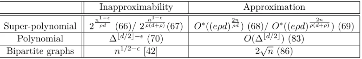
In the second part of the thesis we focus on d-Scattered Set and in particular its (super-)polynomial (in-)approximability: we are interested in the exact relationship between an achievable approximation ratio ρ, the distance parameter d, and the running-time of any ρ-approximation algorithm expressed as a function of the above and the size of the input n. Following this, we consider strictly polynomial running-times and graphs of bounded maximum degree as well as bipartite graphs. Speciﬁcally we show:

• An exact exponential-time algorithm of complexity O∗((ed)2nd ), based on an upper

bound on the size of any solution.

• A lower bound on the complexity of any ρ-approximation algorithm of (roughly) 2n1−ǫρd for even d and 2

n1−ǫ

ρ(d+ρ) for odd d, under the randomized ETH.

• ρ-approximation algorithms of running-times O∗_((eρd)2nρd) for even d and O∗((eρd)

2n

ρ(d+ρ))

for odd d that (almost) match the above lower bounds.

• A lower bound of ∆⌊d/2⌋−ǫ_{on the approximation ratio of any polynomial-time}

algo-rithm for graphs of maximum degree ∆, being the ﬁrst lower bound of this type, as well as an improved upper bound of O(∆⌊d/2⌋_).

• A polynomial-time 2√n-approximation for bipartite graphs and even values of d, that complements known results by considering the only remaining open case. The rest of the thesis is organized in the following way: the theoretical background, deﬁnitions and preliminary results we require are given in Section 2.1, while we discuss related work in Section 2.2; Chapter 3 deals with the (k, r)-Center problem, presenting results published in [67] (originally in [63]) that can also be found in [62]; parameterized results on d-Scattered Set that were originally published in [68] and can also be found in [64] are presented in Chapter 4; (in)approximability results on the same problem are presented in Chapter 5 and can also be found in [65, 66]; a summary of our results and some discussion on open problems may be found in Chapter 6.

(12)

(13)

2

Preliminaries

2.1 Definitions

Computational Complexity background

A decision problem is a language commonly deﬁned on the binary alphabet, i.e. a subset of {0, 1}∗_{. Given some appropriate encoding (a string of binary characters) that fully}

describes an instance, that is a speciﬁc yet abstracted situation, and on which a formal question can be asked with possible answers only of the type “yes” or “no”, the language of a decision problem consists of all such binary strings that encode instances for which the answer to the question is positive and no strings encoding instances for which the answer is negative. A particular instance of a problem is a word on the same alphabet and the word is part of the language only if the word’s answer to the problem’s question is “yes”. A Boolean expression φ is a mathematical formula built on n binary variables xi ∈

{0, 1}, i ∈ [1, n], parentheses and logical operators: conjunction denoted by ∧ (“and”), disjunction denoted by _{∨ (“or”), and negation denoted by ¬ (“not”). A conjunction of} two variables evaluates to 1 if both variables are set to 1, a disjunction of two variables evaluates to 1 if at least one variable is set to 1 and a negation inverts the value of the variable it precedes. An assignment is a string of length n of values for the variables of φ, or a member of{0, 1}n_{. A formula is said to be satisfiable if there is an assignment to}

the variables such that the expression evaluates to 1, i.e. a satisfying assignment. A literal is an appearance of a variable xi in the formula, along with its negation where present.

A formula is in Conjunctive Normal Form (CNF) if it is a conjunction of (usually m) disjunctions of literals, that we refer to as the clauses.

φ = (x1∨ x2∨ x3) ∧ (¬x1∨ x4∨ x5) ∧ (x3∨ ¬x2∨ x6) (2.1)

Formula φ above is in CNF and has n = 6 variables and m = 3 clauses. A satisfying assignment for φ is 001000, as it makes every clause evaluate to 1.

Definition 1. In the Satisfiability problem (SAT), we are given a Boolean expression φ on n binary variables and m clauses in CNF form and are asked if φ is satisfiable.

We let q-SAT refer to the version of SAT where each clause of φ is of size at most q, i.e. φ is a conjunction of m disjunctions, each of at most q literals and still on a total number of n variables. Formula φ above is an instance of 3-SAT, since the maximum number of

(14)

literals in any clause is 3. For a given problem Π and an instance x ∈ Π, a solution (or certificate) is a string y that encodes the part of the instance that justiﬁes the correct answer to the problem’s question as positive. For an instance φ of SAT, a solution y is a string of length n that describes a satisfying assignment.

An algorithm is an unambiguous procedure for identifying a solution (its output) to any given instance of a problem (its input). The number of operations applied or calculations performed by an algorithm is called its running-time and is commonly indirectly expressed as belonging to a set of functions of some appropriate measure of the input’s size, based on the functions’ order and employing the asymptotic notation: for two positive functions f, g, it is f (n)_{∈ O(g(n)) if there exist positive constants c, n}0 such that f(n) ≤ c · g(n) for

all n ≥ n0, while f(n) ∈ o(g(n)) if limn→∞f (n)g(n) = 0. In words, the notation f(n) ∈ O(g(n))

(we also write f(n) = O(g(n))) means that f(n) is upper-bounded by g(n) (up to constant multiplicative factors) and the notation f(n) ∈ o(g(n)) (also f(n) = o(g(n))) means that the rate of growth of f(n) is insigniﬁcant compared to that of g(n).

We say that an algorithm for instances of a problem of size n (for an appropriate deﬁnition of size in each case) is a polynomial-time (resp. exponential-time) algorithm if its running-time expressed as a function of n belongs to O(g(n)) for any polynomial (resp. exponential) on n function g(n). We refer to the set of functions describing the order of the running-time function of an algorithm as the algorithm’s complexity, while a problem’s computational complexity is the best, i.e. the lowest (inclusion-wise) complexity of an algorithm that solves the problem’s worst-case instances, i.e. those instances of the problem that will require the maximum number of calculations/operations in order to be decisively solved.

A reduction is an algorithm that transforms an instance x of a problem Π1 to an

“equivalent” instance y of problem Π2, with appropriate signiﬁcations of equivalence giving

rise to diﬀerent types of reductions, each suited to its particular purpose and the types of problems its function is to relate. Speciﬁcally, for two languages Π1, Π2 encoding decision

problems and deﬁned over alphabets Σ1, Σ2, a many-one reduction from Π1 to Π2 is a

total computable function f : Σ∗

1 → Σ∗2 such that for a word x ∈ Σ∗1, it is x ∈ Π1 if and

only if y ∈ Π2 for y = f(x) ∈ Σ∗2. This means the reduction’s function must compute

instances y of the problem Π2 for which the answer to the question of problem Π2 is “yes”,

if and only if the answer to the question of problem Π1 for the reduction’s input instance

x is also “yes”.

The existence of such an algorithm means that to solve problem Π1, one may use an

algorithm for problem Π2on the output of the reduction. Introducing notions of efficiency,

i.e. limits on allowed running-time functions, we can infer for a problem Π1 reducible to

a problem Π2, that Π1 is as computationally involved, or as eﬃciently solvable as Π2: if

there exists a polynomial-time algorithm for problem Π2 and a polynomial-time many-one

reduction from Π1 to Π2, then the algorithm for Π1 that applies the former on the output

of the latter is also a polynomial-time algorithm. Thus particular types of reductions can be seen to form an equivalence relation (a reflexive and transitive binary relation, a preorder) on a set of problems, whose equivalence classes (sets of equivalence based on this relation) can be used to define complexity classes, i.e. categorizations of problems according to their computational complexity as defined above. From this moreover emerge the computational notions of hardness and completeness: a problem Π is called Γ-hard for a complexity class Γ, under a specific type of reduction, if there exists a reduction of this type from any problem in Γ to Π. If a problem is shown to be Γ-hard and also a member

(15)

of class Γ, then it is called Γ-complete for this type of reduction. Complete problems can thus be naturally seen as representatives of their class.

The most common differentiation in terms of worst-case algorithmic running-time be-tween problems is focused on their identification as polynomial or exponential. This leads to the definitions of the corresponding complexity classes: these problems whose worst-case instances admit an exponential-time algorithm (i.e. O(2p(n)_{) for any polynomial p(n))}

be-long to the class EXPTIME, while the subset of these with a worst-case complexity that is actually O(p(n)) belongs to P. Our interest in differentiating between these types of running-times is not arbitrary: an algorithm of exponential (in the size of the input) complexity is allowed to perform calculations on any possible arrangement of the input’s particular objects of interest and is thus guaranteed to solve most of the interesting com-binatorial problems, while in strictly polynomial running-time an algorithm must be able to find a solution after only a specific number of iterations over the set of input objects. An exponential-time algorithm for instances φ of SAT on n variables can simply calculate the truth value of φ for each of the 2n _{possible assignments to the variables and decide}

whether a satisfying assignment exists if at least one of these makes φ true. Thus we know that SAT belongs to EXPTIME, but since no polynomial-time algorithm has (yet) been discovered for SAT, it is unknown whether SAT also belongs to P.

The class of decision problems whose certificates (of length at most polynomial on the size of the input) can be verified in polynomial time as in fact encoding the part of the input instance that justifies a correct answer to the problem’s question as “yes” is called NP. All problems in P are also in NP. For SAT, an assignment to the variables is such a certificate of length n and the truth value of φ can be verified in polynomial time, meaning SAT is in NP. The famous Cook-Levin theorem states that SAT is also NP-hard, making it the first NP-complete problem. It is generally conjectured that no NP-complete problem is in P, meaning that there is no polynomial-time algorithm for any of these problems, as the existence of a polynomial-time algorithm for one of them would also imply the existence of such an algorithm for all other problems that are reducible to it in polynomial time. This central complexity assumption acts as a starting point for much subsequent theory.

In a more quantitative manner, the Exponential Time Hypothesis (ETH) implies that 3-SAT cannot be solved in (subexponential) time 2o(n) _{on instances with n variables. The}

Strong Exponential Time Hypothesis (SETH) implies that for all ǫ > 0, there exists an integer q such that q-SAT cannot be solved in time (2 − ǫ)n_{on instances with n variables.}

More formally, for each q ≥ 2, let sq be the inﬁmum of the real numbers γ for which

q-SAT can be solved in time O(2γn_{), on instances of size n. Then it is s}

2 = 0 (as 2-SAT is

solvable in polynomial time) and the numbers s3 ≤ s4 ≤ . . . form a monotonic sequence

that is bounded above by 1, meaning they must converge to a limit s_∞. The ETH is the conjecture that sq > 0 for every q > 2, or, equivalently, that s3 > 0. The SETH is the

conjecture that s_∞= 1.

A randomized (or probabilistic) algorithm employs a probability distribution in its decision-making process and is thus not deterministic. Usually this involves additional input in the form of uniformly random bits and the probabilistic error is found in the correctness of the answers given and the validity of produced solutions. The class of decision problems solvable by a probabilistic algorithm in polynomial time with an error probability bounded away from 1/3 for all instances is called BPP. This means for problems in BPP that the algorithms solving them are guaranteed to run in polynomial time, can make random decisions and each of their applications has a probability ≤ 1/3 of giving the

(16)

wrong answer, whether the answer is “yes” or “no”. Note that any number in [0, 1/2) gives rise to the same class since probabilistic algorithms can be applied repeatedly. All problems in P are obviously also in BPP. The relationship between BPP and NP is unknown, yet it is also widely conjectured that NP6⊂BPP. Moreover, a similar conjecture to the ETH can be proposed when considering randomized algorithms.

Some of the most interesting (and applicable) decision problems pose questions related to whether the maximum or minimum attainable value of a given function for a given in-stance is above or below a certain threshold k. Related to each such decision problem is its corresponding optimization problem. The MaxSAT problem asks for an assignment to the variables of instance φ that satisfies the maximum number of clauses, while the related decision version asks if that maximum is ≥ k. Instances of such problems can have any number of feasible solutions, each associated with a particular value of a com-putable objective function defined on it. For MaxSAT, each assignment to the variables of φ is associated with the number of clauses it satisfies. An optimal solution is one for which the problem’s objective function attains its extremal value, being the minimum for minimization and the maximum for maximization problems. An optimal assignment for MaxSATsatisfies the maximum possible number of clauses for the given instance φ. The decision version of MaxSAT is also called NP-hard because an algorithm that solves it can be used to solve SAT, which is NP-complete.

A ρ-approximation algorithm for an optimization problem computes a solution whose value is guaranteed to be at most a multiplicative factor ρ (the algorithm’s approximation ratio) away from the value of an optimal solution for any given instance of the problem. Here we consider ratios ρ > 1 for both minimization and maximization problems and thus the best achievable ratios are always as close to 1 as possible. Formally, for an instance I of an optimization problem Π, let ALG(I) be the value of the problem’s objective function on a solution obtained by a ρ-approximation algorithm and OP T (I) be that of an optimal solution for I. Then it is ρ ≥ OP T (I)

ALG(I) for any instance I of a maximization problem Π,

while in the case of minimization problems it is 1

ρ ≤

OP T (I) ALG(I).

A Polynomial-Time Approximation Scheme (PTAS) is an algorithm that produces a solution whose value is within a factor of (1 + ǫ) from the optimal for a given ǫ > 0 and any instance of an optimization problem in polynomial time. The running-time of a PTAS must be polynomial in the size of the input n for every ﬁxed ǫ. This includes algorithms of running-time O(n1/ǫ_{). The class PTAS contains all problems that admit a}

polynomial-time approximation scheme and is a subset of APX, the class of problems that are approximable to some constant factor. Unless P=NP, there exist problems that are in APX but without a PTAS, so PTAS(APX. The MaxSAT problem is APX-complete and therefore admits no PTAS under the same assumption.

An approximation-preserving reduction from an optimization problem Π1 ⊆ Σ∗1 to

another optimization problem Π2 ⊆ Σ∗2 is a pair of functions f : Σ∗1 → Σ2, g : Σ∗2 → Σ∗1,

where f maps an instance x of Π1 to an instance y of Π2 and g maps a solution for y to

a solution for x. Such algorithms must preserve more than the validity of solutions when reducing from one problem to another, as some guarantee on the worst-case relationship between the value of any solution to that of an optimal solution must also be maintained. What is of interest in this type of transformation between problem instances, especially when considering approximation algorithms with ratios that are functions of the input size n, is the way in which the objective value of valid/optimal solutions relates to the changing size of the instance. The approximation-preserving reductions we present here

(17)

will maintain an equivalence between the objective values of solutions for the input and produced instances, with a marked increase in the size of the latter compared to that of the former.

For a minimization problem Π ⊆ Σ∗_{, a gap-introducing reduction from SAT to Π with}

gap functions f, α is a polynomial-time algorithm that transforms an instance φ of SAT to an instance x ∈ Π, such that:

• if φ is satisﬁable, OP T (x) ≤ f(x), and

• if φ is not satisﬁable, OP T (x) > α(|x|) · f(x). Accordingly, for a maximization problem Π, it must be:

• if φ is satisﬁable, OP T (x) ≥ f(x), and • if φ is not satisﬁable, OP T (x) < _α(|x|)f (x) .

On the hardness side, the gap α(|x|) is the dual notion of the approximation ratio for the algorithmic side: a gap-introducing reduction from SAT shows that it is NP-hard to approximate the problem within a hardness factor of α(|x|), or, equivalently, that the problem admits no polynomial-time α(|x|)-approximation. Note that we maintain α(|x|) ≥ 1 in both cases as we also consider approximation ratios ρ > 1.

A parameterized problem is a language Π ⊆ Σ∗_{× N on ﬁnite alphabet Σ deﬁned along}

with a number characterizing some aspect of the instance and referred to as the parameter. An instance (φ, k) of the decision version of MaxSAT parameterized by the maximum number of simultaneously satisﬁable clauses, i.e. the size k of an optimal solution for φ (generally called the standard parameterization), is a word of the parameterized language if there is an assignment that satisﬁes k clauses of φ.

A parameterized problem Π ⊆ Σ∗ _{× N is Fixed-Parameter Tractable (FPT) if there}

exist a computable function f : N → N, a constant c and a parameterized algorithm that for any instance (x, k) ∈ Σ∗_{× N correctly decides whether (x, k) ∈ Π in time bounded by}

f (k)· O((|x| + k)c_{), that is polynomial in the size of the input (|x| + k). The running-time}

functions f are commonly exponential in the size of the parameter. The complexity class FPT contains all parameterized problems admitting algorithms with running-times of this form. When referring to FPT running-times we mostly use the O∗_{(·)-notation to imply}

omission of factors polynomial in the size of the input n and focus on the part of the running-time expressed by the function f.

For two parameterized problems Π1, Π2⊆ Σ∗× N, a parameterized reduction from Π1

to Π2is an algorithm that runs in time bounded by f(k)·|x1|O(1)and produces an instance

(x2, k2) ∈ Π2 from an instance (x1, k1) ∈ Π1, such that k2 ≤ g(k1), for some computable

function g. A parameterized problem reducible by such a reduction to a problem in the class FPT is also a member of the class. Moreover, if in the above deﬁnition of FPT the constant c is replaced by a computable function g : N → N, we arrive at the deﬁnition of slice-wise polynomial (XP) problems and the corresponding complexity class. This means there exists an algorithm that solves each problem in XP in time that is bounded by f (k)_{· O((|x| + k)}g(k)_{). It is (provably) FPT(XP.}

In parameterized complexity, the class FPT plays a role analogous to that of the class P in classical complexity theory, with XP considered analogous to EXPTIME. Once more, the distinction between ﬁxed-parameter tractable and slice-wise polynomial functions is

(18)

not arbitrary: consider as an example the case of standard parameterization by solution size k, where an XP-time algorithm can compute all the nk _{candidate subsets and decide}

if a solution of this size exists. The analogous role to that of the class NP is played here by the W-hierarchy: each class W[t] in the hierarchy is defined as the class of parameterized problems reducible to a version of SAT defined on boolean circuits of weft t. We omit the definitions of notions related to circuits and provide the definitions of the following parameterized problems instead, each one complete for a level t of the hierarchy.

For a formula φ, the weight of a particular assignment is the number of variables to which the assignment gives a value of 1. The Weighted 2-Satisfiability problem is the version of 2-SAT parameterized by k, where we are asked to ﬁnd a satisfying assignment of weight at most k for an input formula where each clause is of size at most 2. Weighted 2-Satisfiabilityis W[1]-complete. A Boolean formula φ is t-normalized if it is a conjunc-tion of disjuncconjunc-tions of conjuncconjunc-tions and so on, alternating for t levels. Formally, letting A0, B0 be the the set of formulas consisting of a single literal, At is deﬁned for t ≥ 1 as

the set of formulas consisting of the disjunction of any number of B_t−1 formulas and Bt

is deﬁned for t ≥ 1 as the set of formulas consisting of the conjunction of any number of A_t−1 formulas. Bt is then exactly the set of t-normalized formulas. The Weighted

t-Normalized Satisfiability problem is the version of SAT parameterized by k, where we are asked to ﬁnd a satisfying assignment of weight exactly k, while the input formulas are t-normalized. For each t ≥ 2, Weighted t-Normalized Satisfiability is W[t]-complete. It is furthermore FPT=W[0], while every class W[i] is a subset of W[i + 1] and it is conjectured that inclusions are proper. The classes in the W-hierarchy are also closed under parameterized reductions.

For a parameterized problem with parameter k, an FPT approximation scheme (FPT-AS) is an algorithm which, for any ǫ > 0, runs in time O∗_(f(k,1

ǫ)) (i.e. FPT time when

parameterized by k + 1

ǫ) and produces a solution at most a multiplicative factor (1 + ǫ)

from the optimal. We will present approximation schemes with running-times of the form (log n/ǫ)O(k)_{. These can be seen to imply an FPT running-time by the following}

well-known “win-win” argument:

Lemma 2. If a parameterized problem with parameter k admits, for some ǫ > 0, an algorithm running in time O∗((log n/ǫ)O(k)), then it also admits an algorithm running in time O∗((k/ǫ)O(k)).

Proof. We consider two cases: if k_≤√log n then (log n/ǫ)O(k) _{= (1/ǫ)}O(k)_{(log n)}O(√log n)₌

O∗((1/ǫ)O(k)). If on the other hand, k >√log n, we have log n ≤ k2, so O∗((log n/ǫ)O(k)) = O∗((k/ǫ)O(k)).

Graphs

A graph is a pair G = (V, E), where V is a set of idealized abstract objects referred to as the vertices, and E is a set of edges, or pairs of vertices. The edges of a graph deﬁne a symmetric relation on the vertices, the adjacency relation. Two adjacent vertices are also called neighbors. For a graph G = (V, E), n = |V | commonly denotes the number of vertices, m = |E| the number of edges and we also let V (G) := V and E(G) := E. For an edge e = (u, v) = (v, u), the vertices v, u are its endpoints and are said to be incident on e. If the graph is directed its edges are generally called arcs and they are now ordered pairs of endpoints (with tails before heads).1 _{The degree of a vertex v is the number of edges}

1_{Excluding a brief foray in Section 3.4, we only consider undirected graphs here.}

(19)

that v is incident on (the number of its neighbors) and is denoted by δ(v). For a subset X_{⊆ V , we denote by G[X] the graph induced by X, that is the graph whose vertex set is} X and whose edge set consists of all of the edges in E that have both endpoints in X.

A walk of length l is a non-empty sequence x0, . . . , xl of vertices, each consequent pair

xi, xi+1 of which (for i ∈ [0, l − 1]) is connected by an edge (xi, xi+1) ∈ E. A walk is

closed if x0 = xl, while a path is a walk where no two vertices appear twice. A cycle is a

closed walk where no two vertices appear twice, apart from the endpoints. A connected component of a graph is a subgraph in which there is at least one path between any pair of vertices, and which is connected to no additional vertices in the supergraph. The graph is connected if it consists of only one connected component. A subset S ⊂ V is a separator for non-adjacent vertices u, v if the removal of S from G separates u and v into distinct connected components. A tree is a graph in which any two vertices are connected by exactly one path, or, equivalently, a connected acyclic graph, i.e. one that contains no cycles. A forest is a disjoint union of trees.

We denote by dG(v, u) the shortest-path distance from v to u in G, that is the minimum

length of a path in G with endpoints v, u. We may omit subscript G if it is clear from the context. The maximum distance between vertices is the diameter of the graph, while the minimum among all the maximum distances between a vertex to all other vertices (their eccentricities) is considered as the radius of the graph. For a vertex v, we let Nd

G(v) denote

the (open) d-neighborhood of v in G, i.e. the set of vertices at distance ≤ d from v in G (without v), while for a subset U ⊆ V , Nd

G(U) denotes the union of the d-neighborhoods

of vertices u ∈ U. In a graph G whose maximum degree is bounded by ∆, the size of the d-neighborhood of any vertex v is upper bounded by the well-known Moore bound: |NGd(v)| ≤ ∆

Pd

i=0(∆ − 1)i. For an integer q, the q-th power graph of G, denoted by Gq,

is deﬁned as the graph obtained from G by adding to E(G) all edges between vertices v, u∈ V (G) for which dG(v, u) ≤ q.

Two vertices u, v are independent if there is no edge between them, or (u, v) /∈ E. Similarly, a set of vertices is independent if every pair of its vertices is independent (also called a stable set). Conversely, a set of vertices is a clique if every pair of its vertices is connected by an edge. A bipartite graph G = (A ∪ B, E) is a graph whose vertex set is divided into two independent sets A, B and if every vertex of A is connected to every vertex of B the graph is called a bi-clique. We let Kn denote a clique on n vertices (otherwise

known as a complete graph) and Kn1,n2 the bi-clique where |A| = n1 and |B| = n2. It

is well-known that a graph is bipartite if and only if it contains no odd-length cycles. A graph is r-regular if all its vertices are of degree r and speciﬁcally cubic when r = 3. In a chordal graph all cycles on≥ 4 vertices have a chord, i.e. an edge connecting two vertices of the cycle, that is not part of the cycle.

A planar graph can be embedded in the (Euclidean) plane in such a way that its edges intersect only at their endpoints. An edge-weighted graph has a weight function w : E→ N+ _{associated with it that deﬁnes the length of each edge. All above deﬁnitions}

on distance can be extended to accommodate edge weights. The triangle inequality here requires that d(u, v) + d(v, w) ≥ d(u, w) for any u, v, w, where the distance function d obeys the weight function w (which is thus a metric).

For more information on these concepts the reader is referred to the standard text-books: for classical complexity theory see [5, 49, 87, 90], for graph-theoretical notions [16, 19, 39], for approximation algorithms [95, 96], for parameterized complexity [35, 40, 47, 79] and speciﬁcally for the ETH [60, 61].

(20)

Parameters

Treewidth and pathwidth are standard notions in parameterized complexity that measure how close a graph is to being a tree or path (see [10, 11, 14, 71]). Due to their similarity, we focus on treewidth here and only refer to pathwidth when required. A tree decomposition of a graph G = (V, E) is a pair (X , T ) with T = (I, F ) a tree and X = {Xi|i ∈ I} a family

of subsets of V (called bags), one for each node of T , with the following properties: 1) S

i∈IXi = V ;

2) for all edges (v, w) ∈ E, there exists an i ∈ I with v, w ∈ Xi;

3) for all i, j, k ∈ I, if j is on the path from i to k in T , then Xi∩ Xk⊆ Xj.

The width of a tree decomposition ((I, F ), {Xi|i ∈ I}) is max_i∈I|Xi| − 1. The treewidth

of a graph G is the minimum width over all tree decompositions of G, denoted by tw(G). Moreover, for rooted T , let Gi = (Vi, Ei) denote the terminal subgraph deﬁned by node

i _{∈ I, i.e. the induced subgraph of G on all vertices in bag i and its descendants in T .} Also let Ni(v) denote the neighborhood of vertex v in Gi and di(u, v) denote the distance

between vertices u and v in Gi, while d(u, v) (absence of subscript) remains the distance

in G. Path decompositions and pathwidth are similarly deﬁned, with the diﬀerence of T being a path instead of a tree.

In addition, a tree decomposition can be converted to a nice tree decomposition of the same width (in O(tw2 _{· n) time and with O(tw · n) nodes): the tree here is rooted and}

binary, while nodes can be of four types:

a) Leaf nodes i are leaves of T and have |Xi| = 1;

b) Introduce nodes i have one child j with Xi = Xj∪ {v} for some vertex v ∈ V and

are said to introduce v;

c) Forget nodes i have one child j with Xi = Xj\ {v} for some vertex v ∈ V and are

said to forget v;

d) Join nodes i have two children denoted by i − 1 and i − 2, with Xi = Xi−1= Xi−2.

Nice tree decompositions were introduced by Kloks in [71] and using them does not in general give any additional algorithmic possibilities, yet algorithm design becomes consid-erably easier. See Figure 2.1 for examples of tree decompositions.

We will also make use of the notion of clique-width (see [33]): the set of graphs of clique-width cw is the set of vertex-labelled graphs that can be inductively constructed by using the following operations:

1) Introduce: i(l), for l ∈ [1, cw] is the graph consisting of a single vertex with label l; 2) Join: η(G, a, b), for G having cliquewidth cw and a, b ∈ [1, cw] is the graph obtained

from G by adding all possible edges between vertices of label a and vertices of label b;

3) Rename: ρ(G, a, b), for G having cliquewidth cw and a, b ∈ [1, cw] is the graph obtained from G by changing the label of all vertices of label a to b;

(21)

a b c d e f g h i g, h f, g, i e, f, g d, e, g c, e, f a, b, d g, h g g, i f, g, i f, g e, f, g e, f, g e, f, g e, g d, e, g d, e d b, d a, b, d a, b a e, f c, e, f c, e c

Original graph Tree decomposition

Nice tree decomposition

Figure 2.1: Example tree decompositions for a small graph of tw = 2.

4) Union: G1∪ G2 (or G1⊗ G2), for G1, G2 having cliquewidth cw is the disjoint union

of graphs G1, G2.

Note we here assume the labels are integers in [1, cw], for ease of exposition.

A clique-width expression of width cw for G = (V, E) is a recipe for constructing a cw-labelled graph isomorphic to G. More formally, a clique-width expression is a rooted binary tree TG, such that each node t ∈ TG has one of four possible types, corresponding

to the operations given above. In addition, all leaves are introduce nodes, each introduce node has a label associated with it and each join or rename node has two labels associated with it. For each node t, the graph Gt is deﬁned as the graph obtained by applying the

operation of node t to the graph (or graphs) associated with its child (or children). All graphs Gt are subgraphs of G and for all leaves of label l, their associated graph is i(l).

See Figure 2.2 for a small example.

Additionally, we will use the parameters vertex cover number and feedback vertex set number of a graph G, which are the sizes of the minimum vertex set whose deletion leaves the graph edgeless, or acyclic, respectively. Finally, we will consider the related notion of tree-depth [83], which is deﬁned as the minimum height of a rooted forest whose completion (the graph obtained by connecting each node to all its ancestors) contains the input graph as a subgraph. Intuitively, where treewidth measures how far a graph is from being a tree, tree-depth measures how far a graph is from being a star.

We will denote these parameters for a graph G as tw(G), pw(G), cw(G), vc(G), fvs(G), and td(G), and will omit G if it is clear from the context. We also note (avoiding detailed deﬁnitions) that, alternatively, the treewidth tw(G), pathwidth pw(G), tree-depth td(G) and vertex cover vc(G) of a graph G can be deﬁned as the minimum of the maximum clique-size (-1 for tw(G), pw(G) and vc(G)) among all supergraphs of G that are of type chordal, interval, trivially perfect and threshold, respectively. We recall the well-known relations between these parameters, justifying the hierarchy given in Figure 2.3:

(22)

(23)

Notation

We use log(n), ln(n) to denote the base-2 and natural logarithms of n, respectively, while log1+δ(n) is the logarithm base-(1 + δ), for δ > 0. Recall also that log1+δ(n) =

log(n)/ log(1 + δ). The functions ⌊x⌋ and ⌈x⌉, for x ∈ R, denote the maximum/minimum integer that is not larger/smaller than x, respectively.

2.2 Problems and state-of-the-art

Covering problems

We begin with the deﬁnitions of the well-known Dominating Set and Set Cover prob-lems. As here we focus on graph-theoretical formulations, we will mostly consider Domi-nating Set.

Definition 5. In the Dominating Set problem we are given an undirected graph G =

(V, E) and an integer k and are asked to find a subset of vertices D ⊆ V , with |D| ≤ k, such that every vertex not in D has at least one neighbor in D: _{∀v /}_{∈ D : N(v) ∩ D 6= ∅.} Definition 6. Given a universe_{U = {u}1, . . . , un} of elements and a family S = {S1, . . . , Sm}

of subsets of_{U, a cover is a subfamily C ⊆ S of sets whose union is U. In Set Cover,} the input is a pair U, S and an integer k; the question is whether there is a set cover of size k or less.

The Dominating Set problem is NP-complete [49] and cannot be approximated by a factor better than ln n [82]. It is also W[2]-complete parameterized by the size of an optimal solution k and cannot be solved in time f(k) · no(k) _{for any computable f under}

the ETH [35]. Concerning approximability of k in FPT-time, it is shown in [29] that any constant-approximation of the parameterized by k Dominating Set problem is W[1]-hard. Furthermore, the existence of a f(γ(G)) ·|G|(log γ(G))ε/12_{-time algorithm is also ruled}

out, where γ(G) denotes the size of the minimum and assuming the ETH, which on every input graph G outputs a dominating set of size at most 3+εp

log (γ(G))_{· γ(G) for every} 0 < ε < 1. Subsequently, it was shown in [25] that under the Gap-ETH,2 _{no F}

(k)-approximation FPT-time algorithm for Dominating Set parameterized by k exists for any computable function F . Finally, providing an improvement in terms of complexity assumptions, [89] shows there is no F (k)-approximation algorithm for the problem: (a) in FPT-time under FPT6=W[1], (b) in T (k)no(k)_{-time under the ETH, (c) in T (k)n}k−ǫ_-time

for every integer k ≥ 2, under the SETH.

Concerning structural parameters, the problem is solvable in time O∗₍₄cw_{) [15] and}

thus FPT when parameterized by any of the structural parameters we consider here. Speciﬁcally for treewidth, a series of papers had culminated into an O∗₍₃tw_{) algorithm}

[93, 2, 94], while on the other hand, [76] showed that an O∗_{((3 − ǫ)}pw_{) algorithm would}

violate the SETH, where pw denotes the input graph’s pathwidth. Further, [84] notes that the lower bound for pathwidth/treewidth would also imply no (3 − ǫ)cw_{· n}O(1)_-time

algorithm exists for clique-width under the SETH as well, since clique-width is at most 1 larger than pathwidth.

The (k, r)-Center problem is a generalization of Dominating Set (for r = 1):

2_{A stronger assumption than the ETH, stating that no subexponential-time algorithm can distinguish}

between satisfiable 3-SAT instances and those that are not even (1 − ǫ)-satisfiable for some ǫ > 0.

(24)

Definition 7. In (k, r)-Center we are given a graph G = (V, E) and a weight function w : E _{7→ N}+ _{which satisfies the triangle inequality and defines the length of each edge}

and are asked if there exists a set K (the center-set) of at most k vertices of V , so that ∀u ∈ V \ K we have minv∈Kd(v, u) ≤ r, where d(v, u) denotes the shortest-path distance

from v to u under weight function w.

If w assigns weight 1 to all edges we say that we have an instance of unweighted (k, r)-Center. Dealing with (k, r)-Center we allow, in general, the weight function w to be non-symmetric. We also require edge weights to be strictly positive integers but, as we will see (Lemma 43), this is not a signiﬁcant restriction. We will say that a vertex is covered (resp. dominated for r = 1) by a center-set K if it is at distance ≤ r from a vertex u ∈ K. Hardness of (k, r)-Center is inherited from Dominating Set. Moreover, the optimal r cannot be approximated in polynomial time by a factor better than 2, even on planar graphs [45]. In [22], generalizing the previously mentioned results for Dominating Set, it is shown that (k, r)-Center can be solved in O∗_{((2r + 1)}tw_{) (already implied by the}

results of [50]), but not faster assuming the SETH, while its connected variant (i.e. where solutions must consist of connected subgraphs) can be solved in O∗_{((2r + 2)}tw_{), but not}

faster.

For the edge-weighted variant and (unrelated) parameters, [46] shows that a (2 − ǫ)-approximation is W[2]-hard for parameter k and NP-hard for graphs of highway di-mension h = O(log2n), while also oﬀering a 3/2-approximation algorithm of running-time 2O(kh log(h)) _{· n}O(1)_{, exploiting the similarity of this problem with that of solving}

Dominating Set on graphs of bounded vc. For unweighted graphs, [75] provides

eﬃ-cient (linear/polynomial) algorithms computing (r + O(µ))-dominating sets and +O(µ)-approximations for (k, r)-Center, where µ is the tree-breadth or cluster diameter in a layering partition of the input graph, while [41] gives a polynomial-time bicriteria approx-imation scheme for graphs of bounded genus.

Packing problems

We next give the deﬁnitions of the well-known Independent Set (IS) and Set Pack-ing problems. Due to our interest in graph-theoretical formulations we mostly consider

Independent Set.

Definition 8. In the Independent Set problem we are given a graph G = (V, E) and an integer k and are asked to find a subset of vertices I _{⊆ V , with |I| ≥ k, such that every pair} of vertices in I is independent, i.e. there is no edge between them: ∀u, v ∈ I : (u, v) /∈ E.

Definition 9. In the Set Packing problem we are given an integer k, a universe _{U =}

{u1, . . . , un} of elements and a family S = {S1, . . . , Sm} of subsets of U, and are asked

to determine if there is a subfamily S ⊆ S of subsets (a packing), such that all sets in S are pairwise disjoint, while the size of the packing is_{|S| ≥ k.}

The Independent Set problem is NP-complete [49] and inapproximable in polyno-mial time within n1−ǫ _{for any ǫ > 0 [58, 97], but admits a PTAS for planar graphs [6]. For}

graphs of degree bounded by ∆ ≥ 3, Independent Set is APX-complete [86] and not approximable in polynomial time to ∆ǫ _{for some ǫ > 0 [3], but there are greedy (∆ +}

2)/3-approximations [57]. For super-polynomial running-times, any ρ-approximation for the Independent Set problem must require time at least 2n1−ǫ/ρ1+ǫ, almost matching the upper bound of 2n/r _{[26, 36].}

(25)

For a graph G, we let α(G) denote its independence number, i.e. the size of its largest independent set. We also recall here the following result by [26] that some of our later reductions will be relying on (slightly paraphrased, see also [21]), that can be seen as implying the (randomized) ∆1−ǫ_{-inapproximability of Independent Set in polynomial}

time:

Theorem 10 ([26], Theorem 5.2). For any sufficiently small ǫ > 0 and any ∆_{≤ N}5+O(ǫ), there is a randomized polynomial-time reduction that builds from a formula φ of SAT on N variables a graph G of size n = N1+ǫ∆1+ǫ and maximum degree ∆, such that with high probability:

• If φ is satisfiable, then α(G) ≥ N1+ǫ_∆;

• If φ is not satisfiable, then α(G) ≤ N1+ǫ∆2ǫ.

The standard parameterization of the problem by solution size k is W[1]-complete and cannot be solved in time f(k) · no(k) _{for any computable f under the ETH [35].}

Furthermore, [25] shows there is no FPT-time o(k)-approximation, again under the Gap-ETH, improving upon the constant-inapproximability of the problem in FPT-time given in [20, 55]. For all structural parameters considered here the problem is FPT, as there is an O∗₍₂cw_{)-time algorithm [53]. Speciﬁcally for treewidth, the O}∗₍₂tw_{)-time algorithm is}

complemented by a matching SETH-based lower bound of (2 − ǫ)tw_{· n}O(1) _{[35, 76, 94].}

As before, the d-Scattered Set problem is a generalization of Independent Set.

Definition 11. In the d-Scattered Set problem, we are given graph G = (V, E) and a metric weight function w : E _{7→ N}+ that gives the length of each edge and are asked if there exists a set K of at least k selections from V , such that the distance between any pair v, u∈ K is at least d(v, u) ≥ d, where d(v, u) denotes the shortest-path distance from v to u under weight function w.

If w assigns weight 1 to all edges, the variant is also called unweighted. We will also denote by OP Td(G) the maximum size of a d-scattered set in G, thus α(G) = OP T2(G).

The problem is APX-hard for r, d ≥ 3 on r-regular graphs, while there are polynomial-time O(rd−1_{)-approximations [43]. The same paper also shows a polynomial-time}

2-approximation on cubic graphs and a PTAS for planar graphs and every ﬁxed constant d_{≥ 3, extending the algorithm of [6] for Independent Set. For a class of graphs with} at most a polynomial (in n) number of minimal separators (containing chordal graphs), d-Scattered Set can be solved in polynomial time for even d, while it remains NP-hard on chordal graphs and any odd d ≥ 3 [81] (see also [42]).

For the odd values of d, a polynomial √n-approximation is given in [56]. This algorithm is in fact a corollary of a √n-approximation for Set Packing, since there is a correspon-dence between the d-Scattered Set problem for odd values of d and the formulation of independence based on sets [56]: a strong stable set corresponds to a 3-scattered set and is also known as a 2-packing. Given a graph G = (V, E) we can construct a set system (U = V, S = {N(v)∪{v} : v ∈ V }), where the universe consists of the vertices and the sets are deﬁned based on the closed neighborhood of each vertex v, i.e. that also includes v. In this way a strong stable set corresponds to a set of vertices whose closed neighborhoods have no overlap (being thus at distance d ≥ 3), i.e. a set packing of (U, S). Note that this is also equivalent to an independent set in the square graph G2_{, while in general, the}

(2q + 1)-Scattered Set problem is equivalent to Independent Set in (Gq₎2_.

(26)

For bipartite graphs, d-Scattered Set is NP-hard to approximate within a factor of n1/2−ǫ _{and W[1]-hard for any ﬁxed d ≥ 3 [42]. The problem is moreover shown to be}

NP-hard even for planar bipartite graphs of maximum degree 3, while a 1.875-approximation is available on cubic graphs [44]. Furthermore, [48] gives an EPTAS on (apex)-minor-free graphs, based on the theory of bidimensionality, while on a related result an nO(√n)_-time

algorithm exists for planar graphs, making use of Voronoi diagrams and based on ideas previously used to obtain geometric QPTASs (i.e. quasi-polynomial-time approximation schemes, being exponential in poly-logarithmic functions) [80]. Finally, [88] shows that it admits an almost linear kernel (intuitively, the diﬃcult part of a parameterized problem) on every nowhere dense graph class, being a common generalization of several classes including graphs of bounded degree.

In our parameterized reductions we will also make use of k-Multicolored Indepen-dent Set, a well-known W[1]-complete variant that is also unsolvable in time f(k) · no(k) under the ETH [35].

Definition 12. In k-Multicolored Independent Set, we are given a graph G =

(V, E), with V partitioned into k cliques V = V1⊎· · ·⊎Vk,|Vi| = n, ∀i ∈ [1, k], and are asked

to find an S⊆ V , such that G[S] forms an independent set and |S ∩ Vi| = 1, ∀i ∈ [1, k].

(27)

3

On the Structurally Parameterized (k, r)-Center problem

In this chapter we study the (k, r)-Center problem. It is an extremely well-investigated optimization problem with numerous applications. It has a long history, especially from the point of view of approximation algorithms, where the objective is typically to minimize r for a given k [1, 41, 45, 59, 69, 70, 72, 85, 95]. The converse objective (minimizing k for a given r) has also been well-studied, with the problem being typically called r-Dominating Setin this case [24, 30, 50, 77, 91].

Because (k, r)-Center generalizes Dominating Set (which corresponds to the case r = 1), the problem can already be seen to be hard, even to approximate (under stan-dard complexity assumptions). Since this hardness persists when considering the stanstan-dard parameterization of the problem with non-trivial parameterized approximations also pre-cluded, we are strongly motivated to investigate the problem’s complexity when the input graph has some restricted structure.

Our results: Our goal is to perform a complete analysis of the complexity of (k,

r)-Centerthat takes into account this input structure by using the framework of parame-terized complexity. In particular, we provide fine-grained upper and lower bound results on the complexity of (k, r)-Center with respect to the most widely studied parameters that measure a graph’s structure: treewidth tw, clique-width cw, tree-depth td, vertex cover vc, and feedback vertex set fvs. In addition to the intrinsic value of determining the precise complexity of (k, r)-Center, this approach is further motivated by the fact that FPT algorithms for this problem have often been used as building blocks for more elaborate approximation algorithms [37, 41]. Indeed, (some of) these questions have al-ready been considered, but we provide a number of new results that build on and improve the current state-of-the-art. Along the way, we also close a gap on the complexity of the ﬂagship Dominating Set problem parameterized by clique-width. Speciﬁcally, we prove the following:

• (k, r)-Center can be solved (on unweighted graphs) in time O∗_{((3r + 1)}cw_{) (if a}

clique-width expression is supplied with the input), but it cannot be solved in time O∗((3r + 1 − ǫ)cw) for any ﬁxed r ≥ 1, unless the SETH fails.

The algorithmic result relies on standard techniques (dynamic programming on clique-width expressions, fast subset convolution), as well as several problem-speciﬁc observations which are required to obtain the desired table size. The SETH lower