Poland’s accession to the EU : what effects on
transitional dynamics, long run growth and
welfare ?
Sabine Mage
∗This article achieves to assess the impact of Poland’s accession to the European Union (EU) on factor and product markets, household consump-tion, economic growth and also on welfare. To explore the effects of regional integration in this specific transition economy, we implement an applied general equilibrium model with endogenous technological change. A mech-anism through which trade liberalization might change the long run growth is specifically highlighted : the reallocation of resources. We find that adhe-sion may cause the growth rate to fall by inducing to allocate less resources to research and development (R&D) activity, even under the technological diffusion assumption. However, the results suggest that a R&D promotion policy creates a more favorable environment for the regional integration. In this case, trade liberalization stimulates growth and leads to an increase of welfare.
JEL classification : C68; F15; O30; P23
Keywords : Dynamic applied general equilibrium; International trade; Technological transfer; Growth.
∗Université de Paris Dauphine, Département d’Economie, Place du Maréchal de Lattre
1
Introduction
Since the middle of the twentieth century, there has been an important liberalization of world trade taking various forms including unilateral re-ductions in tariff barriers, the formation of free trade areas and customs unions. To what extent has the trade liberalization contributed to the growth of countries ? This question has given rise to an extensive and vigorous debate among both scholars and policymakers. Recent theoretical models investigating the long run effects of economic integration use en-dogenous growth approaches (Grossman and Helpman, 1991 ; Rivera-Batiz and Romer, 1991a,b). This literature looks at the channels through which integration policies might change the rate of technological change, and con-sequently, the growth rate. Most of these policies have a reallocation effect which describes the change in intersectoral resources allocation (between R&D sector and productive sectors) as a consequence of openness. The possibility of international diffusion of technology is also fundamental to understand the evolution of a country’s growth rate. A possible important path for such transmission is the imports of manufactured goods.
Due to the complexity of the endogenous growth theory, this literature necessarily analyzes the long run effects of integration in very aggregated models. According to Baldwin and Forslid (1999, p. 53), it is important to begin work on applied general equilibrium models (AGEM) that introduce endogenous growth : " these efforts should point out the directions in which theoretical models need to be developed in order to explain the reality better ". Moreover, endogenous growth models encounter some difficulties to derive the transitional path following a trade policy implementation and thus, to evaluate the possible adjustment costs necessary to achieve a new steady-state growth path. These elements have, however, crucial repercussions in terms of welfare (Rutherford and Tarr, 2002).
The important theoretical advances of endogenous growth models have led to new empirical research but the relationship between trade liberal-ization and growth is still a matter of controversy. Rodriguez and Rodrik (2000) provide a critique of recent econometric studies based on multiple countries and time periods (Ben-David, 1993 ; Edwards, 1998 ; Sachs and Warner, 1995). This type of analysis is seriously hindered by data limitations about trade policies and is confronted with several questions about imper-fect proxies, influential observations and causality1. Furthermore, when the
results suggest a negative association between trade barriers and growth,
1The relationship between trade liberalization and growth is the relevant question for
economic policy. We should emphasize that the link between changes in trade volumes (that arise from reductions in transport costs or increases in world demand) and growth is a related but distinct question.
most econometric studies conclude in favour of trade openness. However, an increase in the growth rate of output does not necessarily mean an im-provement of welfare.
The paper achieves to investigate the quantitative impact of trade lib-eralization on economic growth but also on welfare. We develop an applied general equilibrium model (AGEM) in which the technical progress is en-dogenous to highlight the mechanisms by which integration could affect the economic performance of a country in the long run. This work is keeping in the last generation of applied modeling whose antecedents are the models of Diao, Roe and Yeldan (1999) and Rutherford and Tarr (2002). We introduce a multisectoral economy to give a detailed evaluation of the reallocation of resources resulting from a change in government policy. The model is solved to obtain the transitional as well as the steady-state equilibria. Thus, we focus on both short run and long run effects of the policy implementation. In particular, the model accounts for the possibility of forgone consumption in the build-up of the capital stock2.
This study concentrates on Poland, the largest transition country set to join the EU. As far you know, examining the consequences of EU member-ship for this specific transition economy with an AGEM introducing tech-nological change has not been performed yet. Poland is a country where domestic spending on R&D was severely cut-off at the beginning of the transition process (the first half of the 1990s) and even now, R&D expen-ditures represent less than one percent of GDP (0.71% in 1997 and 0.59% in 2002). Only around 0.5% of total employment takes part in research ac-tivity. Nevertheless, the perceived relatively high quality of human capital suggests that there is some absorption capacity within the polish economy. The country has opened up and re-orientated its trade flows towards more developed economies. This gave rise to high-technology imports from the West. Thus, one can expect that there has a transfer of innovation and that this transfer could help in productivity improvment3. In the model, we in-troduce cross-border technological spillovers arising from trade and assume a positive linkage between domestic knowledge stock and trading partners knowledge stocks. The trade partners of Poland are aggregated into three re-gions : European Union, East countries (Hungary, rest of Central European Associates, former Soviet Union) and the rest of the world.
We distinguish two sets of policies. First, we investigate the impact of regional integration without and with the technological diffusion assumption.
2The gains from trade liberalization will be overestimated in a comparative static
analyse before and after trade liberalization (Rodrik, 1997).
3In particular, Coe, Helpman and Hoffmaister (1997) and Bayoumi, Coe and Helpman
(1999) provide an empirical study of the technological transfer between developed and developing countries.
The model is calibrated for the year 1997 while the integration of Poland into the EU is effective in 2004. Thus, we consider a pre-announced trade policy after seven years. We simulate a removal of tariffs on imports from EU and a reduction from the others trade partners4. Our major finding is that regional integration leads to allocate less resources in R&D sector and consequently, the growth rate decreases. This trade policy results in a welfare loss in the long run. Second, we study the consequences of regional integration when the government also introduces a subsidy on R&D activies. We show that the R&D promoting policy allows to enlarge the absorptive capacity of the country and to benefit from international technological spillovers.
The plan of the article is as follows. Section 2 introduces the theoretical structure of the model. Section 3 presents the model’s data sources and the calibration method. Section 4 reports and analyses numerical results with respect to European integration policy. Section 5 concludes.
2
The model
The model of Diao and alii (1999) applied to Japan, takes into account important theoretical advances of the growth literature in a very desaggre-gated economy. Following them, we provide a detailed description of the R&D accumulation and of the sectoral production. In this article, the gov-ernement and the fiscal policy variables play also a fundamental role in the adhesion process.
In the model, the accumulation of knowledge (the creation of new ideas) is the source of growth. Following Romer (1990), technological progress takes the form of an expansion in the number of differentiated intermedi-ate capital goods. These intermediintermedi-ate goods, which embody the technical progress undertaken in the R&D sector, enter in the production of the final goods. Three sectors are considered :
- a R&D sector in which the production of knowledge exhibits constant returns to scale
- an intermediate sector which produces differentiated capital under im-perfect competition (the sector consists of individual firms so that each firm only produces one variety of intermediate good with a monopoly rent)
- a final good sector which produces exports and domestic goods under constant returns to scale. The production intended to the domestic market is used both for consumption and investment. This sector is desaggregated into several sub-sectors of final goods to allow the study of the reallocation of ressources in the economy. The economy is open to the final goods and imports are distinguished by their geographical origin.
4
The mathematical presentation of the model and a detailed glossary are given in the appendix A (page 19).
2.1
The R&D sector
The aggregate R&D production function is the following :
A(t + 1) − A(t) = B(t)Lrd(t)γLHrd(t)γHT rd(t)γTA(t) (1)
This sector produces new blueprints (A(t + 1) − A(t)) using inputs of labour (Lrd), human capital (Hrd), and a non-human factor (T rd). The produc-tivity coefficient is denoted by B. The environment is perfectly competitive : γL+ γH + γT = 1. The research sector is relatively more intensive in human capital. The production of new designs also depends on the stock of knowledge accumulated in the past (A). This specification induces that innovators can use the available stock of knowledge (due to its public good nature) to build a new design. The stock of knowledge accumulates from the spillovers of previous ideas, that is, this stock acts as a positive external-ity. These public good aspects of knowledge create economy-wide increasing returns.
As recent studies show the influence of cross-border technological spillovers on growth (Lee, 1995 ; Coe and Helpman, 1995 ; Coe and alii, 1997), we also introduce a linkage between domestic R&D stock and trading partners R&D stocks. According to empirical evidence, the effectiveness of research B, is a positive function of knowledge of trade partners. Following Diao et alii (1999), the productivity coefficient can be written in this linear form :
B(t) = (1 + sp(t))B0 (2)
where B0is the initial coefficient. We assume that the international spillovers
coefficient sp depend on the stock of knowledge of each region rg, Af (rg), weighted by the share of high-tech imports from the region rg. This share is denoted by δ(rg) :
sp(t) = φX
rg
δ(t, rg)Af (t, rg)
The parameter φ indicates in which extent the technological transfer affects the domestic R&D productivity.
The technological diffusion assumption is not without critics. Keller (1998) analyzes findings by Coe and Helpman (1995) on the link between the elasticity of domestic productivity and foreign R&D stocks. The results suggest that randomly created trade patterns (rather than true bilateral trade patterns proposed by Coe and Helpman) give also, and often larger,
positive R&D spillovers. In response to Keller, Coe and Hoffmaister (1999) show that with alternative random weights (not simple averages with a ran-dom error as in Keller (1998)), the estimated international R&D spillovers are nonexistent.
2.2
The intermediate sector
The intermediate sector produces capital goods which enter in the pro-duction of the final goods. In this sector, a firm h can produce, at any point of time, a quantity kbh of only one variety of capital goods and charges the
price pkh. This production is allowed by the payment of a fixed cost (the
price of a patent) to the R&D sector. For each period, there exists A inter-mediate goods and thus A firms in the sector. Innovations are protected by a patent and must provide a rent to innovators. The monopoly firms have a forward looking behaviour. The value of a patent is then defined as the present discounted value of monopoly profits that the holder of the patent can extract. At the equilibrium, to assure the investment in blueprints, the non-arbitrage condition must hold :
v(t + 1) + π(t) = (1 + r(t))v(t) (3) where v denotes the patent price, π is the profit of each monopolist and r, the interest rate. The condition stipulates that the expected returns from investment must be comparable with those from holding a safe asset such as bank deposits.
All monopoly firms are symmetrical (kbh = kb) and bear the same price
(pkh= pk) :
pk(t) = r(t)Cmk(t) αk
(4) where Cmk(t) is per unit material cost of each capital variety. The mark-up (1/αk) is derived from the inverse demand of final producers adressed to the
monopolist5. To sum up, the quantity of differentiated capital at any point
of time is the number of varieties (A) multiplied by the quantity produced of each (kb). We assume that the depreciation rate of capital varieties is zero.
The total production of differentiated capital is a Cobb-Douglas function of investment in each final good i denoted by ID(i) :
[(A(t + 1)kb(t + 1)] − [A(t)kb(t)] = Bk
Y
i
ID(t, i)η(i) (5) where η(i) is the share of investment in good i in the total value of investment and Bk is a shift parameter.
2.3
Production and sales of final goods
The economy operates with ten final output sectors : agriculture, min-erals, food manufacturing, intermediate materials (petroleum, coal ucts, plastic products, ferrous metals...), light industry (textiles, wood prod-ucts...), transport equipment, electronic equipment, other machines and equipment, other manufactured goods (metal products, motor vehicles and parts) and services. Following the O.E.C.D. classification (2003a), we make a distinction between "high and low technological sectors"6.
The production of each final good i is written as : Y (t, i) = M in
(
Bf(i)L(t, i)αL(i)H(t, i)αH(i)T (t, i)αT(i) A R h=1 kh(t, i)αk; DI(t, i) ) (6) where Y (i) is the output, Bf(i) is a shift parameter, L(i) is the labour
input, H(i) is the human capital input, T (i) is a non human factor7 and kh(i) is the employment of the hth type of specialized intermediate good.
In the symetric case, the capital factor is written as A(t)k(t, i)αk. The other
intermediate demand of sector i (intermediate demand in all final goods) is denoted by DI(i).
The value added function specifies constant returns to scale in all inputs together (αL(i) + αH(i) + αT(i) + αk = 1). The share parameter αk is
the same in all sectors to ensure a balanced growth path8. Technological progress takes the form of an expansion in A, the number of specialized intermediate goods. To focus on the study of economic growth through productivity, the supplies of labour, human capital and non human factors ressources are inelastic and held constant over time. The high-tech sectors are relatively more intensive in high skilled labour and are used in most part for investment in the intermediate sector. All production factors are perfectly mobile in the economy, but immobile internationally. The relevant policy variables in this model are the tariff rates on imports.
Outputs of all final sectors are demanded in several different ways. First, each final good i is produced for sale in the domestic market and foreign market. The magnitude of sales at home and abroad is determined by rel-ative prices. This is an Armington-style differentiation of products in the
6
The different equipment sectors are considered as high-tech sectors.
7The introduction of the input T is used to adjust polish data to the theoretical model.
Without its "fudge factor", a steady-state growth path cannot be reproduced (cf. section 3). The possibility to accumulate the factor T would be satisfactory but in this case, two sources of growth are introduced in the model.
8"Without this assumption, the importance of one of these sectors would decline over
time until that sector enventually vanished from the long run equilibrium." Grossman and Helpman (1991, p.146).
export market. A constant elasticity of transformation (CET) function re-lates the composite output level Y (i), in a given period, to domestic and exports sales respectively denoted by D(i) and E(i). Firms producing final goods maximize profit under the constraint :
Y (t, i) = BY(i) · µ(i)E(t, i) 1+ee(i) ee(i) + (1 − µ(i))D(t, i) 1+ee(i) ee(i) ¸ ee(i) 1+ee(i) (7) In this equation, BY(i) is a shift parameter, µ(i) is the share parameter for
foreign goods and ee(i) is the elasticity of the CET.
Final goods serve also as intermediate inputs of production in each of the ten final sectors. They meet the demand for final consumption by the households and the consumption of the government. Lastly, high-tech goods and services are employed in investment to produce capital varieties.
2.4
The foreign sector
Imported goods by Poland are country source-specific and are considered to be imperfect substitutes in consumption for the domestically produced goods. The home country’s demanders of final goods (the final sector, the intermediate sector, the households and the government) choose domestic goods D(i) and foreign goods M (i, rg) into each composite CC(i) at min-imum cost according to a contant substitution function (CES), that is an Armington function. For a given period :
CC(t, i) = BC(i) " X rg ν(i, rg)M (t, i, rg) em(i)−1 em(i) + (1 −X rg ν(i, rg))D(t, i) em(i)−1 em(i) # em(i) em(i)−1 (8) In this equation, BC(i) is a shift parameter, ν(i, rg) is the share parameter
for foreign good from region rg and em(i) is the CES elasticity. To keep the model realistic for polish economy, we introduce the capacity to borrow internationally.
The evolution of the foreign debt (F D) is described by the following equation :
F D(t + 1) = (1 + r(t))F D(t) − BC(t)
where BC denotes the trade balance for each period and r the interest rate of the economy.
2.5
Consumer behaviour and government revenue
We consider a representative household, with perfect foresight and forward-looking behaviour, which maximizes an intertemporal utility function (U )
under a wealth accumulation constraint. The total wealth includes the present value of returns to primary factors and the revenue of monopoly firms. The intertemporal utility depends on a Constant Relative Risk Aver-sion instanteneous utility function :
U = ∞ X t=0 µ 1 1 + ρ ¶t CT (t)1−σ1 − 1 1 −1σ (9) The rate of time preference is denoted by ρ and the intertemporal elasticity of substitution by σ. Aggregate consumption in a given period CT is a Cobb-Douglas function of consumption of different final goods i :
CT (t) =Y
i
C(i)β(i) (10)
where β(i) is the fixed expenditure share of good i in the value of total consumption.
The government provides public goods and services at an exogenous level. The impact of public provision on consumer welfare is not taken into account. The government resources include tariffs (T XM ), household income taxes (T XH), final output taxes (T XYi) and consumption taxes
(T XV Ai). The ad valorem tariffs which are the relevant policy instruments
in our study are exogenous specified variables whereas consumption taxes (value added taxes) could be exogenously or endogenously determined to as-sure a constant budget for the government. The consumption tax is applied both to domestic and imported goods.
On the expenditure side, the government subsidizes the research activity to reduce the cost of inputs employed in the R&D sector (T XS) (or subsi-dizes the final sector to reduce the price paid by employers of differentiated capital and stimulates their demand).
Y G(t) =X i T XY (t, i)+T XH(t)+X i T XM (t, i)+X i T XV A(t, i)−T XS(t) where Y G denotes the government revenue.
2.6
Social welfare
This article analyzes the welfare impact of the economic policy implemen-tation from the intertemporal utlity function. The welfare change is mesured by the equivalent variation over the horizon which is defined as a percent of the consumption present value of benchmark steady-state. Two welfare equations must be introduced. First, we define the intertemporal welfare when any economic policy is undertaken :
ΩS(t) = P∞ t=0 µ 1 1 + ρ ¶tà CT (t)1−σ1 − 1 1 −1σ !
where CT denotes the consumption for each period without shock in the economy. Second, we define the intertemporal welfare after the policy sim-ulation : Ω(t) = P∞ t=0 µ 1 1 + ρ ¶tà CT (t)1−1σ − 1 1 −σ1 !
where CT is the household consumption for each period after the shock. The part of consumption which must be given to the household to compensate him for a possible cutting down of its consumption, is determined from the following equation : Ω(t) = P∞ t=0 µ 1 1 + ρ ¶tà (CT (t) + ϕ)1−1σ − 1 1 −σ1 !
where ϕ is the equivalent variation. The policy implementation improves the consumer welfare when ϕ > 0.
3
Benchmark data and calibration
To illustrate the mechanisms of the model, we study the impact of Poland’s adhesion into the EU. Our model is then specified and calibrated to polish data (the reference year is 1997). We construct a benchmark steady-state equilibrium before any simulations and then compare the results of the new equilibrium path of variabes after trade policies with the corresponding val-ues in the initial steady-state model. Our model runs for 100 annual periods to assure a convergence.
The data about production, consumption, investment and trade are drawn primarily from the Global Trade Analysis Project database version 5 (2002). The GTAP data about protection in Poland reveal that tariff rates are very different among the final sectors. For example, ad valorem tariff protecting food industry are very high (around 70%) while in the case of electronic equipement tariff are relatively small (around 13%).
Further information about R&D expenditures and capital knowledge stock, growth rate, time preference rate and intertemporal elasticity of substitution is needed. Long run series data about R&D expenditures for Poland and its trade partners are provided by O.E.C.D. (2003b,c). We then construct the knowledge stock for Poland and for each region considered in the model. From the R&D expenditures data, used as proxies of knowledge production, we construct knowledge stocks with the inventory perpetual method. The initial steady-state growth rate is the average of rates on the last twenty years (given by the polish central office of statistics GUS, 2003). The values given to the time preference rate and the intertemporal elasticity of substitution are these used in most dynamic AGEM and are very closed from these chosen by Lucas (1988).
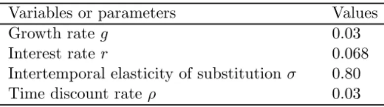
The calibration of the model is based on the fact that initial data depict a steady-state growth path. Wendner (1999) proposes a method to calibrate dynamic AGEM for non steady-state situations in the case of an exogenous technical progress. This procedure leads to a more realistic interpretation of the benchmark data for transition or developing countries. But it implies to make some shocks in the benchmark independently of the policy scenarios. In our model, any simulation modifies the long run growth rate because of the endogenous technological change. That is the reason why it is very dif-ficult to apply the Wendner’s method. Thus, the steady-state assumption allows us to calibrate the model (see the appendix B page 26 for a presen-tation of the calibration strategy). The table 1 gives some key benchmark values.
Table 1: Selected benchmark values
Variables or parameters Values
Growth rate g 0.03
Interest rate r 0.068
Intertemporal elasticity of substitution σ 0.80
Time discount rate ρ 0.03
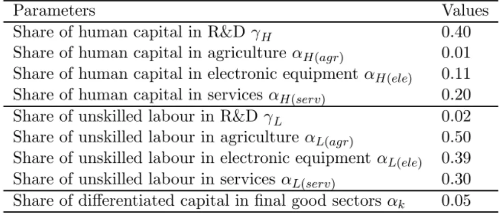
GTAP provides a distinction between unskilled and skilled labour but do not provide information about R&D personnel and high skilled labour. Thus, in this field, others data sources are also needed. Data on labour and high skilled labour inputs in the R&D sector are given by O.E.C.D. (2003b,c). The perfect competition assumption allows to adjust the quantity of the non human factor. It’s more difficult to separate data on labour input from high skilled labour input in the final goods sector. The distinction has been allowed by data of the International Organization of Labour (I.L.O.) on professional occupation categories. The calibration allows to translate input data to model parameters. In the table 2, some function production parameters are provided.
We can observe that the share of differentiated capital in final ouput production is small. This is due to the small research activity in Poland and that is the reason why the non human factor plays an adjustment role.
4
Model results
In this section, we first provide a quantitative assessment on the link between regional integration and economic performance without and with the technological diffusion assumption. Second, we simulate a subsidy on
Table 2: Selected share parameters in production functions
Parameters Values
Share of human capital in R&D γH 0.40 Share of human capital in agriculture αH(agr) 0.01
Share of human capital in electronic equipment αH(ele) 0.11 Share of human capital in services αH(serv) 0.20
Share of unskilled labour in R&D γL 0.02 Share of unskilled labour in agriculture αL(agr) 0.50 Share of unskilled labour in electronic equipment αL(ele) 0.39
Share of unskilled labour in services αL(serv) 0.30 Share of differentiated capital in final good sectors αk 0.05
R&D activies and investigate the impact of regional integration in this new environment.
4.1
Regional integration
The first simulation under consideration is the Poland’s accession into the European Union which supposes : a removal of tariffs on EU imports ; a reduction of tariffs on high technological imports from East and rest of the world countries to eighty percent ; a reduction of tariffs on low technological imports from East and rest of the world countries to thirty percent. We first assess the question of regional integration without cross-border technological spillovers. The regional integration is a pre-announced trade policy which takes place in 2004 (seven years after the reference year). To keep the government revenue constant after the trade liberalization, a value added tax on each final good i is introduced. We consider an uniform tax rate of 4%.
In the regional integration scenario, the economy is open both to high-tech and low-high-tech goods. These sectors are respectively intensive in human capital and low skilled labour. Thus, this trade policy leads to simultaneous opposite effects on the allocation of resources in the economy. The results depend on three main effects. First, reducing the protection on low-tech goods leads to a relative increase in the real prices of high-tech goods. The high technological sectors benefit from an increase of their output and conse-quently resources are diverted to the these manufacturing sectors and away from R&D production. The rate of knowledge accumulation being the ulti-mate source of growth in the model, the growth rate slows down. Second, reducing the protection on high-tech goods leads to the opposite effects that these described previously and implies a faster long run growth rate. On a theoretical point of view, the net effect of the trade policy is indeterminate.
Third, an increase of value added taxes on both domestic and imported goods to compensate the government for the lowering of tariff revenue leads to an increase of composite prices which is unfavorable to the consumption and investment.
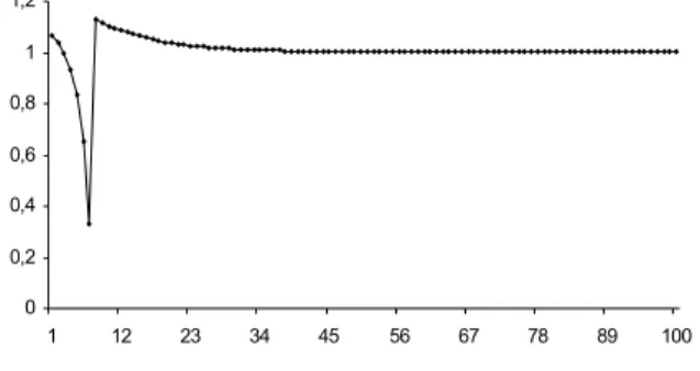
Our results concerning the effects of regional integration on Polish growth rate are presented in figure 1 which gives the time-path of the growth rate relative to the baseline steady-state equilibrium (benchmark =1). During the transition, we can observe a decrease of the growth rate before the regional integration and a sudden rise the year the tariff cut is implemented. We recall that the policy is implemented only after seven years. That is the reason why most of the adjustments take place at the moment of the regional integration9. Nethertheless, with the pre-announcement, the agents
enter in anticipation of the rade liberalization. Our results suggest that households prefer reduce their consumption during the period preceding the trade policy. Thus, the growth rate declines from 1997 to 2003. The year of the trade liberalization, the economy increases imports and the consumption rises owing to temporary trade deficits.
Figure 1: Growth rate (relative to the benchmark steady-state)
0 0,2 0,4 0,6 0,8 1 1,2 1 12 23 34 45 56 67 78 89 100
In the long run, the growth rate recovers its benchmark value (3%). Thus, this scenario doesn’t allow to durably change the economic perfor-mance of the Polish economy. What is driving these results is the follow-ing. Given the initial structure of tariffs and importations volumes, the trade liberalization leads to a relative increase of high-tech goods composite prices. This increase in the costs of capital investment affects negatively the monopoly firms : the production of new capital varieties declines. In the new steady-state, the quantity of each capital variety produced by monopoly firms is lowered to 3.1%.
The regional integration also affects the allocation of resources among
9
In the model of Rutherford and Tarr (2002), a delayed implementation of trade liber-alization doesn’t allow to reduce adjustment costs as well.
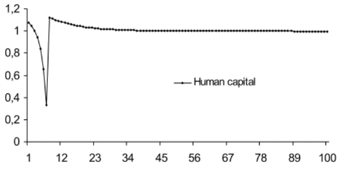
the sectors in the economy. In the model, R&D activities compete for human capital with the sectors producing final high-tech goods. One the one hand, if trade liberalization results in a loss of resources in the R&D sector, the rate of growth slows down. On the other hand, an increase of resources in the final sectors boosts the manufacturing activity and the demand of differentiated capital is more important in the long run. The figures 2 and 3 depict the change of human capital resource in the R&D sector and the transportation equipment sector respectively. Through this example, we can observe that when the human capital is diverted to R&D activity, final high-tech goods sectors take advantage of this reallocation and conversely. Figure 2: Human capital in RD activity (relative to the benchmark steady-state) 0 0,2 0,4 0,6 0,8 1 1,2 1 12 23 34 45 56 67 78 89 100 Human capital
Figure 3: High skilled labour in transportation equipment (relative to the benchmark steady-state) 0,9 0,95 1 1,05 1,1 1,15 1 12 23 34 45 56 67 78 89 100
High s killed labour
The results described in figure 2 and figure 3 depend on the effects of policy implementation on the relative rental rates of primary resources. Our experiments reveal that the patent price v decreases (rises) as the relative price of human capital (wH
wL) decreases (rises). This finding strengthens the
results of Diao and alii (1999). During the seven periods before the regional integration, the relative average rental rate of human capital is below its
benchmark value and decreases until the trade liberalization is implemented. The patent price changes in the same way. This implies a slowing down in the production of new blueprints and a decrease of human capital quantity employed in the research activity.
In this scenario of pre-announced regional integration, the consumption equivalent variation ϕ decreases by 2.1% of the present value of consumption over the one hundred year horizon. This result is explained for a great part by the increase of composite high-tech goods prices which leads to the increase of blueprints costs and consequently to the slow down in the production of new varieties.
We assess now the question of trade liberalization in the case of techno-logical diffusion. We conduct the same experiment than previously (regional integration and an uniform value added tax system) but allow for interna-tional knowledge spillovers.
The importations of high-tech goods allow the technology transfer. We calibrate the R&D productivity parameter such that an increase in the share of high-tech imports from each region rg increases the productivity of do-mestic research. Our results show that the consumption equivalent variation is also negative. Each period, the total consumption is reduced by 1.7% re-spect to the benchmark value in the case of a low international spillover coefficient sp (the elasticity of domestic R&D to foreign knowledge is closed to the elasticities values estimated by Coe and Helpman, 1995).
In this simulation, the share of investment good import is practically unchanged. This result is due to the regional integration which implies to open the Polish economy both to low-tech and high-tech imports. The trade liberalization of low technological sectors decreases the share of high-tech imports in the total volume of importations. It is the reason for the absence of spillovers effects. Thus, in this scenario, taking into account the international knowledge spillovers doesn’t affect the long run growth rate.
4.2
Subsidy to R&D activity and regional integration
In this model of endogenous growth, knowledge enters into production in two distinct ways. On the one hand, a new design allows the production of a new intermediate good that can be immediately used in the final sector. It follows that a new idea also increases the total stock of knowledge. On the other hand, innovators can use the available stock of knowledge due to its public good nature and build a new design. The stock of knowledge accumulates from the spillovers of previous ideas, that is, this stock acts as a positive externality. This specification implies a market failure : each producer of differentiated capital cannot appropriate the blueprint of others
producers due to the property rights but each new variety creates a more efficient production of blueprints.
To better understand this mechanism, we encourage domestic R&D ac-tivity by introducing an ad valorem subsidy (s) to the cost of inputs em-ployed by the R&D sector. We can also consider a subsidy to the employers of differentiated capital and stimulates the demand for varieties. Here the scenario under consideration is the regional integration coupled with a sub-sidy which implies a reduction of the cost of factors in the R&D sector. The subsidy rate is chosen at the level of 5% which represents a relative small expenditure for the government.
The outcomes of this simulation on the growth rate are presented in the figure 4. A subsidy to producers of R&D output allows to reduce the costs of primary resources in this sector. But in the same time, the trade liberalization diverts resources from the R&D activity.
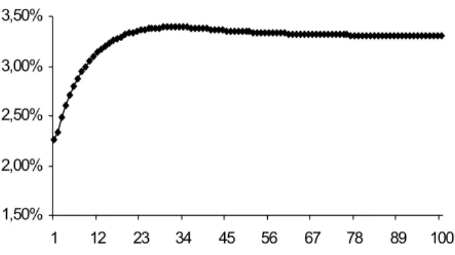
Figure 4: Growth rate
1,50% 2,00% 2,50% 3,00% 3,50% 1 12 23 34 45 56 67 78 89 100
In the short run, the shift of primary resources is to the detriment of the blueprints production. It is the reason why the growth rate slows down in the first periods. However, from the year 2006, the growth rate recovers its benchmark value and reachs 3.33% to the new steady state. In the long run, the shifts of resources are much larger than previous scenarios. To the new steady state, the amount of human capital increases by 7.1% in the R&D activity.
In response to ressource reallocation, the production of final goods in-crease in the short run and especially the first year. In the transporta-tion equipment sector, the output increases by 4% the first period and in the minerals sector, by 5.15%. Along the transition path, the final output declines but remains above the benchmark level because of the increased number of varieties. The subsidy to the R&D activity allows to encourage
the knowledge accumulation and the production of blueprints. Due to the increased number of differentiated capital employed in the final production, the productivity of primary factors increases and reduces the effect of the reallocation of resources.
In this scenario, we observe that the consumption equivalent variation ϕ is positive. Each period, the total consumption increases by 7.2% respect to the benchmark value. This result is due to the more rapid accumulation of knowledge than in the reference scenario. At the year 2006, the households begin to enjoy the gains from faster growth.
In this context of R&D promotion policy, the impact of Poland’s adhesion into the European Union on growth is positive. But what is driving this result is the R&D domestic policy (which induces a better reallocation of resources and to increase the technological absortive capacity) rather than the trade liberalization policy.
5
Conclusion
In this paper, we propose an applied general equilibrium model with en-dogenous growth to assess the impact of Poland’s accession to the European Union on economic performance and social welfare. We focus on a particu-lar mechanism through which trade liberalization could affect the long run growth rate : the reallocation of ressources. Thus, the model is multisectoral to allow the study of the reallocation of resources between the R&D sector and the manufactured sectors. Moreover, we obtain both the transitional and the steady-state equilibria to evaluate the costs of a possible forgone consumption to achieve a new steady-state.
The results suggest that Polish adhesion to the European Union has a negative impact on welfare even with the technological diffusion assumption. The reason is that the trade liberalization is applied both to high-tech and low-tech imports and implies opposite effects on the reallocation of resources. The fiscal policy has also important repercussions on the prices charged in the economy. The results illustrate the crucial importance of encouraging the domestic private R&D activity. The subsidy to the costs of primary factors employed in the R&D sector creates a more favorable environment for the regional integration.
In this paper, to focus on the resources reallocation, trade liberalization concerns the final goods sectors which operate under the perfect competition conditions. The liberalization of the intermediate sector and the entry of foreign capital varieties is an other channel through which international integration could affect the economic performance of a country. In the case
of the Polish’s adhesion, the entry of foreign differentiated capital induces the study of the link between foreign direct investment and growth.
Appendix A.1 : Mathematical presentation of the model
Final output and factor demands
Y (t, i) = Bf(i)L(t, i)αL(i)H(t, i)αH(i)T (t, i)αT(i)A(t)k(t, i)αk (A.1)
wL(t)L(t, i) = pva(t, i)αL(i)Y (t, i) (A.2)
wH(t)H(t, i) = pva(t, i)αH(i)Y (t, i) (A.3)
wT(t)T (t, i) = pva(t, i)αT(i)Y (t, i) (A.4)
(1 − τk)pk(t)A(t)k(t, i) = pva(t, i)αkY (t, i) (A.5)
Intermediate sector v(t + 1) + π(t) = (1 + r(t))v(t) (A.6) pk(t) = r(t)cmk(t) αk (A.7) π(t) = (1 − αk)pk(t)kb(t) (A.8) kb(t) =X i k(t, i) (A.9) [A(t + 1)kb(t + 1)] − [A(t)kb(t)] = Bk Y i
ID(t, i)η(i) (A.10)
Knowledge accumulation, spillovers ans factor demands
A(t + 1) − A(t) = B(t)Lrd(t)γLHrd(t)γHTrd(t)γTA(t) (A.11)
B(t) = (1 + sp(t))B0 (A.12) sp(t) = φX rg δ(t, rg)Af(t, rg) (A.13) δ(t, rg) = P ts pwm(t, ts)M (t, ts, rg) P ts pc(t, ts)ID(t, ts) (A.14) wL(t)Lrd(t) = (1 + s(t))γLv(t)(A(t + 1) − A(t)) (A.15)
wH(t)Hrd(t) = (1 + s(t))γHv(t)(A(t + 1) − A(t)) (A.16)
wT(t)Trd(t) = (1 + s(t))γTv(t)(A(t + 1) − A(t)) (A.17)
pe(t, i) = pwe(t, i)er
1 + te(t, i) (A.18)
pva(t, i) = py(t, i)(1 − ty(t, i)) −X
j
aijpc(t, j) (A.19)
py(t, i)Y (t, i) = pe(t, i)E(t, i) + (1 + tva(t, i))pd(t, i)D(t, i) (A.20)
pc(t, i)CC(t, i) = X
rg
pwm(t, i)er(1 + tmr(t, i, rg))(1 + tva(t, i))M (t, i, rg)(A.21) +(1 + tva(t, i))pd(t, i)D(t, i) (11)
Foreign exchanges Y (t, i) = BY(i) · µ(i)E(t, i) 1+ee(i) ee(i) + (1 − µ(i))D(t, i) 1+ee(i) ee(i) ¸ ee(i) 1+ee(i) (A.22) E(t, i) D(t, i) = µ pe(t, i) (1 + tva(t, i))pd(t, i) ¶ee(i)µ 1 − µ(i) µ(i) ¶ee(i) (A.23) CC(t, i) = BC(i) " X rg ν(i, rg)M (t, i, rg) em(i)−1 em(i) + (1 −X rg ν(i, rg))D(t, i) em(i)−1 em(i) # em(i) em(i)−1 (A.24) M (t, i, rg) D(t, i) = µ
pwm(t, i)er(1 + tva(t, i))(1 + tmr(t, i, rg)) (1 + tva(t, i))pd(t, i) ¶−em(i) 1 −P rg ν(i, rg) ν(i, rg) −em(i) (A.25) BC(t) =X i er à pwe(t, i)E(t, i) − pwm(t, i)X rg M (t, i, rg) ! (A.26) Household consumption CT (t + 1) = µ 1 + r(t + 1) 1 + ρ ¶σµ pct(t) pct(t + 1) ¶σ CT (t) (A.27)
CT (t) =Y i C(t, i)β(i) (A.28) System demand DIT (t, i) =X j aijY (t, j) (A.29)
pc(t, i)ID(t, i) = η(i)cmk(t){[A(t + 1)kb(t + 1)] − [A(t)kb(t)]} (A.30)
pc(t, i)C(t, i) = β(i)pct(t)CT (t) (A.31) pc(t, i)CG(t, i) = θ(i)CGT (t) (A.32) Saving and revenue
YM(t) = (1−th(t)) £ wL(t)L(t) + wH(t)H(t) + wT(t)T (t) + pk(t)A(t)kb(t) + T R ¤ (A.33) SM(t) = YM(t) − pct(t)CT (t) (A.34) YG(t) = T XH(t) + X i T XY (t, i) +X i T XM (t, i) +X i T XA(t, i)(A.35) −T XS(t) − T XK(t) −X i T XE(t, i) − T R
T XY (t, i) = ty(t, i)py(t, i)Y (t, i) (A.36) T XH(t) = th(t)YM(t) (A.37)
T XM (t, i) = erX
r
tm(t, i, r)pwm(t, i)M (t, i, r) (A.38)
T XA(t, i) = tva(t, i)pd(t, i)D(t, i)+erX
r
(tva(t, i)tm(t, i, r)pwm(t, i)M (t, i, r)) (A.39) T XS(t) = s(t)v(t)[A(t + 1) − A(t)] (A.40) T XK(t) = τk(t)pk(t)kb(t) (A.41)
T XE(t, i) = te(t, i)pe(t, i)E(t, i) (A.42) SG(t) = YG(t) − CGT (t) (A.43)
Domestic absorption
Factor markets equilibrium X i L(t, i) + Lrd(t) = L (A.45) X i H(t, i) + Hrd(t) = H (A.46) X i T (t, i) + Trd(t) = T (A.47)
Borrowing and debt
F D(t + 1) = (1 + r(t))F D(t) − BC(t) (A.48) W (t + 1) = (1 + r(t))W (t) + Y M (t) − pct(t)CT (t) (A.49) P D(t + 1) = (1 + r(t))P D(t) − SG(t) (A.50) Investment-saving equilibrium SM(t) + SG(t) − BC(t) = X i
pc(t, i)IV (t, i) + v(t)(A(t + 1) − A(t)) (A.51)
Growth rate
g(t) = A(t + 1) − A(t)
Appendix A.2 : Glossary
¥ Endogenous variables Prices
py(i) Final good i output price pd(i) Domestic price for good i pva(i) Value added price for good i pe(i) Export price for good i pc(i) Composite price for good i pk Variety price
wL Unskilled labour rental price
wH Skilled labour rental price
wT Non human factor rental price
cmk Marginal cost of one monopolist
v Patent price r Interest rate
pct Aggregate consumption price Output and factors demands
Y (i) Sectoral output for good i D(i) Domestic supply for good i
L(i) Unskilled labour demand from sector i H(i) Skilled labour demand from sector i T (i) Non human factor demand from sector i A Knowledge stock
k(i) Variety demand quantity from sector i
kb Variety quantity produced by each monopolist π Monopolist profit
Lrd Unskilled labour demand from research sector
Hrd Skilled labour demand from research sector
Trd Non human factor demand from research sector
Γ Productivity coefficient in knowledge accumulation sp Spillover coefficient
w(rg) Share of high-tech imports from region rg Demand
C(i) Household consumption for good i CT Household aggregate consumption CG(i) Government consumption for good i IV (i) Investment demand for composite good i DIT (i) Intermediate demand for good i
CC(i) Quantity of composite good i Foreign exchanges
M (i, rg) Imports of good i from region rg E(i) Exports of good i
BC Trade balance F D Foreign debt Saving and revenue
W Household wealth YM Household revenue SM Household saving YG Government revenue SG Government saving P D Public debt
T XY (i) Ouput taxes revenu T XH Direct taxes revenu
T XA(i) Consumption taxes revenu T XM (i) Tariff revenu
T XS Research subsidies
T XK Intermediate good subsidies T XE(i) Export subsidies
Growth rate
g Transitional growth rate ¥ Exogenous variables
Exogenous variables for economic policy tm(i, rg) Tariffs for good i from region rg ty(i) Sectoral final good output tax i th Household revenu tax
tva(i) Value added tax for good i s Research subsidy
τk Intermediate good subsidy
te(i) Export subsidy Others exogenous variables
pwm World price of imports for good i pwe World price of exports for good i er Exchange rate
Af(rg) Knowledge stock for region rg
CGT Total government consumption (value) L Unskilled labour supply
H Skilled labour supply T Non human factor supply ¥ Parameters
Utility function
ρ Time preference rate
σ Intertemporal elasticty of substitution Production functions
αL(i) Share parameter for factor L in value added function
αH(i) Share parameter for factor H in value added function αT (i) Share parameter for factor T in value added function
αk Share parameter for factor k(i) in value added function
γL Share parameter for factor L in knowledge production γH Share parameter for factor H in knowledge production γT Share parameter for factor T in knowledge production Bf(i) Shift parameter in value added function
Bk Shift parameter in intermediate goods production function
φ International spillover elasticity Demand
η(i) Share parameter in intermediate goods production function β(i) Share parameter in household demand
φ(i) Share parameter in government demand aij input-output coefficient
Armington functions
em(i) Elasticity of substitution in CES function BC(i) Shift parameter in CES function
ν(i, rg) Share parameter in CES function
ee(i) Elasticity of substitution in CET function BY(i) Shift parameter in CET function
Appendix B : Calibration strategy
To compute both the transitional and the steady-state equilibria, we "detrend" all of the variables which grow in the long run by the steady-state growth rate. The quantities variables grow in the long run at the same rate that the growth rate of blueprints excluding the quantity of each variety, the profit of monopolists and the supplies of skilled labour, unskilled labour, non human factor. Hence, the only prices which grow in the long run are the rental prices of these factors.
For instance, we calibrate the interest rate r from the dynamic equation for consumption (equation A.27 in the appendix A) :
CT (t + 1) = µ 1 + r(t + 1) 1 + ρ ¶σµ pct(t) pct(t + 1) ¶σ CT (t) which becomes after we have detrended the consumption variable :
(1 + gLT)gCT (t + 1) = µ 1 + r(t + 1) 1 + ρ ¶σµ pct(t) pct(t + 1) ¶σ g CT (t)
where gLT is the long run growth rate and gCT denotes the detrended
con-sumption level. With the steady-state ascon-sumption, we obtain for the refer-ence path : 1 + g0 = µ 1 + r0 1 + ρ ¶σ
where g0 is the initial steady-state growth rate. Now, we can calibrate r0
the benchmark value for the interest rate. The same procedure is applied for all of the values unknowed at the benchmark.
References
[1] Baldwin, R.E. et Forslid, R. (1999) Putting growth effects in com-putable equilibrium trade models. In R.E Baldwin et J. Francois (eds.), Dynamic Issues in Applied Commercial Policy Analysis (pp. 44-84). Cambridge, New-York and Melbourne : Cambridge University Press. [2] Barro et Sala-I-Martin (1996) Economic Growth. McGraw-Hill, Inc. [3] Ben-David, D. (1993) Equalising exchange : trade liberalization and
income distribution. Quaterly Journal of Economics 153, 653-679. [4] Coe, D. T. et Helpman, E. (1995) International R. & D. spillovers.
European Economic Review 39, 859-887.
[5] Coe, D. T., Helpman, E. et Hoffmaister, A.W. (1997) North-South R&D spillovers. Economic Journal 107 (440), 134-149.
[6] Coe, D. T. et Hoffmaister, W. A. (1999) Are There International R. & D. Spillovers Among Randomly Matched Trade Partners ? A Response to Keller. IMF Working Paper 99/18.
[7] Diao, X., Roe, T. et Yeldan, E. (1999) Strategic policies and growth : an applied model of R&D-driven endogenous growth. Journal of Devel-opment Economics 60, 343-380.
[8] Edwards, S. (1998) Openness, productivity and growth : what do we really know ? Economic Journal 108, 383-398.
[9] Grossman, G. et Helpman, E. (1991) Innovation and Growth in the Global Economy. Cambridge, the MIT Press.
[10] G.T.A.P. (2002) Global Trade, Assistance, and Production : The GTAP5 Data Base. Center for Global Trade Analysis, Purdue Uni-versity.
[11] G.U.S. (2003) Concise Statistical Yearbook of Poland. Office Central de Statistiques Polonais.
[12] I.L.O. (2004) LABORSTAT- Base de données sur les statistiques du travail, Organisation Internationale du travail.
[13] Keller, W. (1998) Are international R. & D. spillovers trade-related ? Analyzing spillovers among randomly matched trade partners. Euro-pean Economic Review 42 (8), 1469-1472.
[14] Lee, J.W. (1995) Capital goods imports and long-run growth. Journal of Development Economics 48, 91-110.
[15] Lucas, R. (1988) On the mechanics of economic development. Journal of Monetary Economics 22 (1), 3-42.
[16] O.C.D.E (2003a) Tableau de bord de la STI (Science, Technol-ogy, Industrie), Organisation de Coopération et de Développement Economique.
[17] O.C.D.E. (2003b) Principaux Indicateurs de la Science et la Tech-nologie, volume 2003 édition 03, Organisation de Coopération et de Développement Economique.
[18] O.C.D.E. (2003c) Statistiques de base de la Science et Technologie, vol-ume 2003 édition 01, Organisation de Coopération et de Développement Economique.
[19] Rivera-Batiz L.A. et Romer, P. (1991a) Economic integration and en-dogenous growth. Quaterly Journal of Economics, 106 (2), 531-556. [20] Rivera-Batiz, L.A. et Romer, P. (1991b) International trade with
en-dogenous technological change. European Economic Review 35 (4), 971-1005.
[21] Rodriguez, F. et Rodrik, D. (1999) Trade Policy and Economic Growth : A Skeptic’s Guide to the Cross-National Evidence. NBER Working Paper series, 7081.
[22] Romer, P. (1990) Endogenous technological change. Journal of political Economy 98, S71-S102.
[23] Rutherford, T. et Tarr, D. (2002) Trade liberalization, product vari-ety and growth in a small open economy : a quantitative assessment. Journal of International Economics 56, 247-272.
[24] Sachs, J. et Warner, A. (1995) Economic reform and the process of global integration. Brookings Papers on Economic Activity 1, 1-118. [25] Wendner, R. (1999) A calibration procedure of dynamic CGE
mod-els for non-steady state situations using GEMPACK. Computational Economics, 13, 265-287.