On the determinants of food price volatility
Kuhanathan ANO SUJITHAN† Sanvi AVOUYI-DOVI†* Lyes KOLIAI†
This version: February 15, 2014 Abstract
In this paper, we investigate the determinants of price volatility for six major food commodities from January 2001 to March 2013. In the recent literature, real economic activity, biofuel production, oil prices and financial markets indicators are commonly considered to be the main drivers of price volatility. We identify and analyse the relationships between these macroeconomic and financial factors and our commodities within a Bayesian multivariate framework. Then we assess the effect of each factor on food volatility in the recent period. We show that, although results depend on food commodities, they are consistent with those available in the latest studies. In other words, the two most recent surges in food prices do not significantly change the dynamics of these prices. We have also performed an analysis of the effects of certain shocks on food commodity markets. These exercises do not reveal the existence of coherent groups of food commodities.
JEL Classification: C32, Q11, Q18
Keywords: Food price volatility, BVAR model, volatility spillovers
The views expressed in this paper are those of the authors and do not necessarily reflect those of the Banque de France or Paris-Dauphine University. The authors would like to thank Advani Renuka for her help and useful comments and Virginie Fajon for her assistance. Any remaining errors are theirs.
(†) Paris-Dauphine University
(*) Banque de France and Paris-Dauphine University.
2
1. Introduction
There is a growing body of literature that seeks to identify the channels through which changes in volatility affect the real economy (Bloom 2009). For instance, Fernandez-Villaverde et al. (2011a, b) use a structural model to suggest one channel through which changes in real interest rate volatility or a fiscal volatility shock can affect open economies. At least for major industrialised countries, It is also well-documented, that the volatility of monetary policy shocks and that of supply and demand shocks fluctuate. These findings raise questions over the effects of the volatility of other macroeconomic factors, and especially the effects of food price volatility on global and local economies.
The increase in nominal food prices and its inflationary consequences have mainly penalised poor populations, notably in developing countries. These populations derive a large proportion of their income from trade in basic food products (Hernandez et al. 2011). As a result, food security and food price stability have become major concerns for most governments throughout the world.
The recent unanticipated shocks on commodity markets have revived interest in the dynamics of commodity prices, and especially in that of food commodities. Indeed, the large peaks in international food prices observed between 2007 and 2008 and from 2010 to 2011 were unexpected for most observers. One of the consequences of the recent behaviour of commodity markets was to incite the G20 and the BRICS to address these issues at their 2011 annual meetings (Gilbert, 2010). Note that the impact of volatility in certain macroeconomic factors on economic activity could be examined via an extended version of the SVAR model. Indeed, it is possible to combine a SVAR model with a stochastic volatility model which enables the introduction of time-varying variances. By imposing a dynamic interaction between the endogenous variables of the SVAR and the time-varying variances, it is possible to directly assess the effects of volatility on some aggregates (Mumtaz and Theodoridis, 2012; Lemoine and Mougin, 2010).
In general, fundamental factors such as market conditions or climatic events are usually considered to be the key explanatory variables of food price changes. However, the recent macroeconomic and financial turmoil has prompted the emergence of new studies which have tested different determinants of food price volatility (Cooke and Robles, 2009; Gilbert, 2010; Roache, 2010; Tadese et al. 2013).
To be more precise, let us list some of the usual explanatory factors cited for food price volatility: Production indicator, especially in emerging countries (China and India). For example, Gilbert
(2010) stresses that strong economic growth in these countries has a significant impact on food price volatility. Moreover, sharp positive changes in the output of these countries have led to shifts in dietary patterns towards meat and dairy products. One of the consequences of this has been an increase in demand for grains (von Braun, 2011);
Demand indicator for biofuels (Abbot et al. 2008; Mitchell, 2008; Chakravorty et al., 2010); Exchange rates. Shocks to the price of financial assets, and especially to currencies, can affect the
income of food commodity producers. The recent depreciation of the US dollar (USD) is a good illustration of this (Abbot et al., 2008);
Oil prices. Fluctuations in oil prices can lead directly to variations in food prices (Alhalith, 2010), and can also influence the dynamics of food prices via biofuel prices (Busse et al., 2010). In addition, there can exist volatility spillovers between the oil and food commodity markets (Nazlioglu et al., 2013; Du et al., 2011);
Speculation on commodity futures markets. Robles et al. (2009), Gilbert (2010) and Shi and Arora (2012) all investigate this factor. However, its effect is more or less ambiguous (Wright, 2011); Trade restrictions (Headey, 2011; Martin and Anderson, 2012).
These effects are not easy to identify or to assess; they can also generate an iterative process that causes feedback effects. For instance, a drought in Russia or a bad monsoon in India may increase food prices through fundamental market forces, and this can in turn be reinforced by financial speculation or trade restrictions.
As a result, we have chosen to implement a multivariate framework which allows us to take these feedback effects into account in the empirical model.
The remainder of this paper is organised as follows. Section 2 provides a general overview of volatility and the recent developments in food commodity markets. Section 3 describes the model and provides the comments on the empirical results. Section 4 discusses some of the policy implications of food commodity volatility. Section 5 concludes.
2. Recent developments in food commodity markets
2.1. The commodities under review
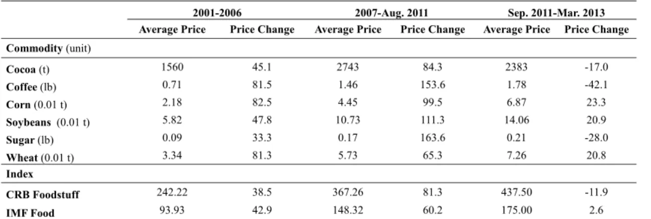
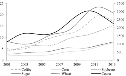
The price of most food commodities almost doubled between 2006 and July 2008. Indeed, all the synthetic indicators (see Figure 1B) show a sharp increase in the food price index over this period. For example, the CRB foodstuff spot index rose by around 50% in 2007-2008. A similar pattern can be seen between mid-2010 and December 2011. Thus, from 2007 to August 2011, almost all food commodity prices doubled (see Table 1). On an individual level, however, (i.e. when we scrutinize the different components of the synthetic indicators), some discrepancies appear between the two periods. For instance, rice was the most expensive grain during the phases of huge expansion from 2006 to 2008, but exhibited a lower price than most grains in 2011. Symmetrically, the price of sugar was significantly lower than its historical average during the first episode, but reached an all-time high in 2011. In addition, since September 2011, prices have remained high, but some (cocoa, coffee, and sugar prices) have decreased while others have continued to increase. The trends in food commodity prices obtained by the application of the Hodrick Prescott filter confirm these results (see Figure 1A).
Table 1. Food commodity prices*
2001-2006 2007-Aug. 2011 Sep. 2011-Mar. 2013 Average Price Price Change Average Price Price Change Average Price Price Change Commodity (unit) Cocoa (t) 1560 45.1 2743 84.3 2383 -17.0 Coffee (lb) 0.71 81.5 1.46 153.6 1.78 -42.1 Corn (0.01 t) 2.18 82.5 4.45 99.5 6.87 23.3 Soybeans (0.01 t) 5.82 47.8 10.73 111.3 14.06 20.9 Sugar (lb) 0.09 33.3 0.17 163.6 0.21 -28.0 Wheat (0.01 t) 3.34 81.3 5.73 65.3 7.26 20.8 Index CRB Foodstuff 242.22 38.5 367.26 81.3 437.50 -11.9 IMF Food 93.93 42.9 148.32 60.2 175.00 2.6
* Average nominal prices in USD and price change in percentage points. Sources: Datastream and authors’ calculations.
In this paper, we focus on cocoa, coffee, corn, soybeans, sugar and wheat. Coffee is one of the most traded food commodities in the world; it was ranked in the top 10 of exported and imported food commodities in 2011. Even though cocoa does not play an important role in the global food market,
4 we have decided to include it in our set of variables as the income of some developing countries, especially in Africa (Ivory Coast, Ghana, Nigeria, etc.), is heavily dependent on cocoa exports.
Figure 1A. Food price trends
Sources: Datastream and authors’ calculations.
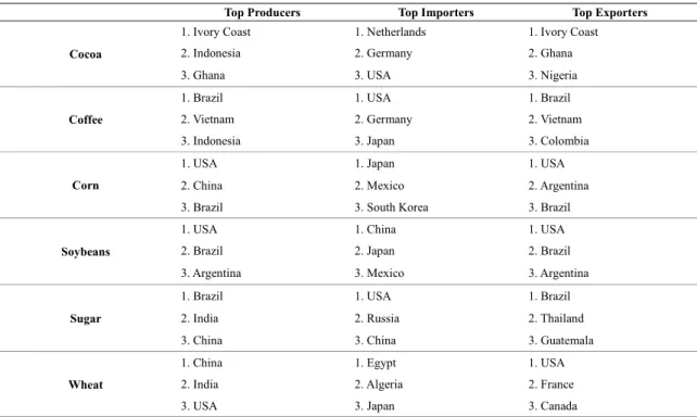
Grains are a major food staple, especially in developing countries. They also play a key role in the global food market (see Table 2). In addition, they serve as animal feed and are even used as a currency in some regions. We study the following grains: (i) wheat, which is the most important grain produced and consumed in temperate regions; (ii) corn, which is cultivated in temperate and tropical regions, is the key basic food in eastern and southern Africa and also serves to produce biofuels, and (iii) soybeans, which are cultivated in many regions around the globe and are used to produce oil and cattle feed.
Figure 1B. Food commodity indices
Source: Datastream. 0 500 1000 1500 2000 2500 3000 3500 0 5 10 15 20 25 2001 2003 2005 2007 2009 2011 2013 Coffee Corn Soybeans Sugar Wheat Cocoa
We excluded rice from our framework, even though it is the staple food in Asia, Central and West Africa and the Caribbean. Rice consumption and production are very different from those of other grains and food commodities, in that the major producers are also the largest consumers. Shocks in the rice markets also have a low correlation with those in other grains markets, and the main Asian rice producers (India and China) can stabilise rice prices for consumers through trade restrictions and stockpiling policies (Timmer, 2010). This type of procedure is harder to set up in other food commodity markets. Thus, the movement of rice prices is almost unrelated to changes in the prices of other grains. Furthermore, derivatives markets for rice are not sufficiently liquid or developed (Gilbert and Morgan, 2010).
Table 2. Main actors in the global food commodity markets
Top Producers Top Importers Top Exporters
Cocoa
1. Ivory Coast 1. Netherlands 1. Ivory Coast 2. Indonesia 2. Germany 2. Ghana
3. Ghana 3. USA 3. Nigeria
Coffee
1. Brazil 1. USA 1. Brazil
2. Vietnam 2. Germany 2. Vietnam
3. Indonesia 3. Japan 3. Colombia
Corn
1. USA 1. Japan 1. USA
2. China 2. Mexico 2. Argentina
3. Brazil 3. South Korea 3. Brazil
Soybeans
1. USA 1. China 1. USA
2. Brazil 2. Japan 2. Brazil
3. Argentina 3. Mexico 3. Argentina
Sugar
1. Brazil 1. USA 1. Brazil
2. India 2. Russia 2. Thailand
3. China 3. China 3. Guatemala
Wheat
1. China 1. Egypt 1. USA
2. India 2. Algeria 2. France
3. USA 3. Japan 3. Canada
Sources: FAO and USDA. 2.2. Data
We use monthly data covering the period from January 2001 to March 2013. The dataset on food commodity prices is compiled from Datastream; all prices are nominal prices in USD. We use the prices quoted by the US Department of Agriculture (USDA) for “Corn No.2 Yellow”, “Wheat No.2 Soft” and “Soybeans No.1 Yellow”. We also include the price for Brazilian coffee as quoted by Thomson-Reuters. Prices for cocoa and sugar are provided respectively by the International Cocoa Organization (ICCO) and the International Sugar Organization (ISO). Finally, we calculate monthly data using last-day-of-the-month figures.
In order to take into account a wide variety of potential determinants of food price volatility, we look at financial market factors, macroeconomic factors, biofuel market indicators and oil prices.
First, due to its leading role in equity markets, we consider the Standard and Poor’s 500 stock index as the main factor describing global financial markets.
6 For global macroeconomic factors, we use monthly global GDP. As emerging economies seem to have a strong influence on food price volatility, we decided to disentangle the GDP of emerging economies from that of the rest of the world. This allows us to examine the effect on food volatility of GDP growth in advanced countries and of GDP growth in emerging countries (as quoted by the IMF). Moreover, global GDP can be replaced with the US Industrial Production Index (IPI) in the analysis. The Merrill Lynch Biofuels spot price index acts as a global indicator of market conditions for biofuels. Oil prices are introduced into our analysis through monthly spot prices for both WTI and Brent crude oil.
First-order log-differences are sufficient to remove any unit root in the series. Descriptive statistics of the dataset are reported in Appendix 1.
2.3. Volatility measurement
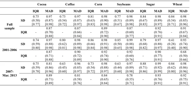
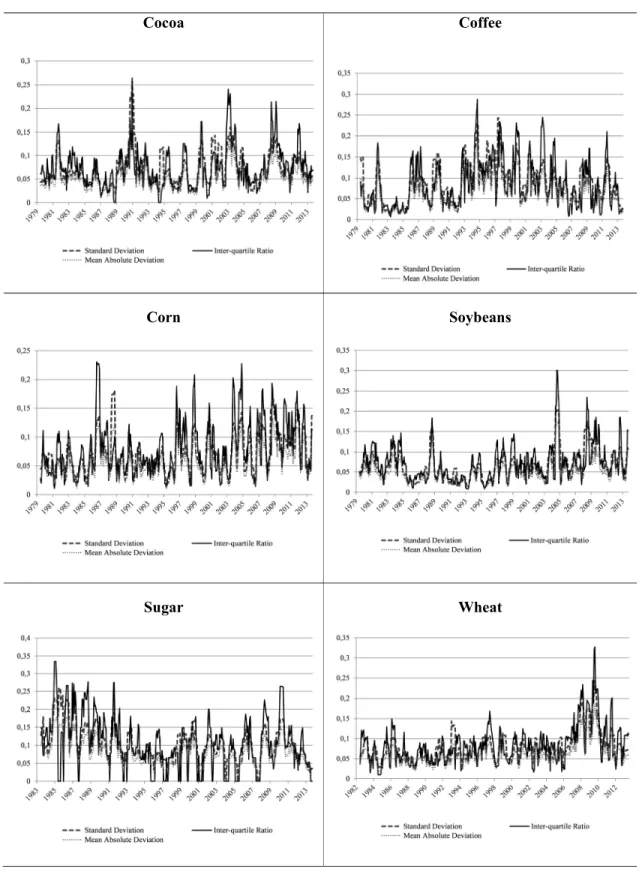
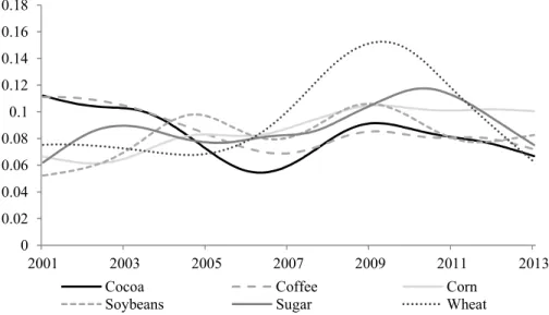
Volatility plays a key role in finance and economics. As a result, we have noted explosive growth in the number of methodological and empirical studies of volatility dynamics. Recent research has focused on finding ways to improve the measurement and understanding of volatility (Todorov et al., 2014). There are several options available for measuring food price volatility: standard dispersion indicators can be used (e.g. standard deviation (SD), the inter-quartile ratio (IQR), the rolling mean absolute deviation (MAD), etc.); alternatively, it is also possible to derive a volatility indicator from a GARCH or stochastic volatility framework or from nonparametric statistics based on high-frequency option data. In this paper, we focus on standard dispersion measures. We compute these measures on a 6-month rolling basis for our food commodities. Three-month and 12-month rolling measures are also performed for consistency purposes. Figure 2 and Table 3 show that all three measures display similar patterns for each commodity, and that the correlations are relatively high. In particular, Kendall’s tau and Spearman’s rho indicate a high degree of concordance in the dispersion measure for each food price. We also observe that volatility peaks are not simultaneous inside the set of food commodities and that not all were more volatile during the 2007-2008 and 2010-2011 prices surges. In addition, whatever the measure of food price volatility, the indicator of dispersion is always time varying. For example, the correlation between SD and IQR is strongly time-dependent while that between SD and MAD is almost stable. Volatility clearly follows an upward trend from 2007 to 2009 or 2010, but has been stable or decreasing since 2011 (Figure 3).
Table 3. Dependence structure of food volatility measures*
Cocoa Coffee Corn Soybeans Sugar Wheat
IQR MAD IQR MAD IQR MAD IQR MAD IQR MAD IQR MAD
Full sample SD 0.75 (0.58) [0.77] 0.97 (0.87) [0.98] 0.73 (0.54) [0.72] 0.97 (0.87) [0.97] 0.81 (0.63) [0.83] 0.98 (0.90) [0.98] 0.77 (0.51) [0.67] 0.98 (0.89) [0.98] 0.84 (0.67) [0.83] 0.98 (0.89) [0.97] 0.84 (0.54) [0.71] 0.98 (0.85) [0.96] IQR - 0.87 (0.70) [0.88] - 0.87 (0.66) [0.84] - 0.89 (0.72) [0.90] - 0.87 (0.60) [0.77] - 0.92 (0.76) [0.91] - 0.91 (0.67) [0.84] 2001-2006 SD 0.74 (0.59) [0.80] 0.97 (0.88) [0.98] 0.80 (0.62) [0.81] 0.98 (0.89) [0.98] 0.86 (0.66) [0.84] 0.98 (0.91) [0.98] 0.85 (0.50) [0.65] 0.99 (0.88) [0.98] 0.79 (0.68) [0.82] 0.97 (0.88) [0.97] 0.41 (0.28) [0.40] 0.93 (0.74) [0.90] IQR - 0.87 (0.71) [0.88] - 0.90 (0.72) [0.89] - 0.92 (0.74) [0.90] - 0.92 (0.60) [0.76] - 0.90 (0.77) [0.91] - 0.68 (0.50) [0.66] 2007- Mar. 2013 SD 0.75 (0.59) [0.78] 0.81 (0.86) [0.96] 0.63 (0.45) [0.60] 0.96 (0.85) [0.97] 0.73 (0.54) [0.72] 0.98 (0.88) [0.97] 0.63 (0.44) [0.60] 0.97 (0.89) [0.98] 0.88 (0.71) [0.86] 0.99 (0.92) [0.99] 0.84 (0.62) [0.80] 0.98 (0.86) [0.96] IQR - 0.89 (0.71) [0.89] - 0.81 (0.58) [0.76] - 0.84 (0.65) [0.84] - 0.78 (0.55) [0.71] - 0.93 (0.76) [0.91] - 0.92 (0.75) [0.91]
Linear correlations are given in the first line. Kendall’s tau and Spearman’s rho values are displayed in parentheses and square brackets respectively. With the exception of wheat, all series are stationary at the 10% significance level at least. All dependence or concordance statistics are significant at 1%.
Figure 2. Price volatility dynamics of food commodities
Cocoa Coffee Corn Soybeans Sugar Wheat
8 Source: Datastream and authors’ calculations.
Figure 3. Food price standard deviations from trend (HP filter)
Source: Datastream and authors’ calculations.
3. The main determinants of food price volatility
3.1. The model
We use a dynamic multivariate framework to investigate the links between the volatility of certain food prices and their main determinants. To do this, we implement a type of multivariate model from the vector autoregressive (VAR) literature (Sims, 1980).
Thus, if y represents the 1 vector of the endogenous variables, the model is an order autoregressive representation of the vector y. In this paper it has the form
L y c+ε for t=1, …, T, (1)
Where is the sample size, L is a polynomial matrix in the lag operator L of order and a vector of error terms i.i.d. 0 , Σ . The likelihood function can be derived from the sampling density ℙr y| , Σ , where .
However, we face an identification problem in this framework due to the values of M and p. This can be overcome by making artificially strong assumptions to reduce the number of parameters, or finding some appropriate theoretical reasons which could allow us to reduce this number. The theoretical-based reduction of the number of parameters leads to the structural vector autoregressive (SVAR) model. The use of the SVAR model can be justified if one knows the underlying theory. In other words, the representation of the state of the economic theory requires a high degree of uncertainty. An alternative solution is provided by the Bayesian vector autoregressive (BVAR) model (Litterman, 1986). This approach allows us to introduce Bayesian prior information into the VAR framework. Indeed, according to Litterman (1986) or Sims and Zha (1998) for example, the BVAR does not require judgmental adjustments and it generates a complete multivariate probability distribution for outcomes. To understand and forecast the endogenous variables, it is worth noting that the BVAR approach is based on the view that information about the future can be found across a wide spectrum of economic data. In addition, it is now common knowledge that a BVAR model can be used for
0 0.02 0.04 0.06 0.08 0.1 0.12 0.14 0.16 0.18 2001 2003 2005 2007 2009 2011 2013
Cocoa Coffee Corn
10 forecasts, IFR analysis and a structural analysis (Banbura et al. 2010). We propose estimating a BVAR model to identify the main determinants of food price volatility.
To do this, we need to define prior distributions for the parameters and draw posterior distributions within a Bayesian approach.
To estimate the vector of parameters in the previous equations, we need to set prior distributions for the unknown parameters i.e. both and Σ. According to Kadiyala and Karlsson (1997) or Sims and Zha (1998), there are many prior distributions with different characteristics, one of which is Litterman’s prior distribution, also referred to as the Minnesota prior distribution. This was one of the first methods used for estimating BVAR models and is still frequently used. Although Kadiyala and Karlsson (1997) have found that there are other prior distributions which are preferable, we essentially focus on the Minnesota prior distribution in this version of our paper.1 This is because the Minnesota prior is simple to implement. Moreover, we do not perform forecasts in this paper. Indeed, the performance of the Minnesota prior can be questionable if forecasts are made.
3.2. A brief overview of Minnesota prior distributions
We can refer to Litterman (1986), Kadiyala and Karlsson (1997), Sims and Zha (1998) or Del Negro and Schorfheide (2010) for more detailed presentations of Litterman prior distributions. As is common in these approaches, we replace Σ with an estimate Σ. The problem is then how to set priors for the parameter . Let:
~ , (2)
where and define the priors for . Thus, the corresponding posterior is given by
~ , (3) where Σ ⨂ (4) and Σ ⨂ y (5) where … and 1, .
Σ is assumed to be a diagonal matrix with elements 1, … , and where is the OLS estimate of the error variance in the th equation of the VAR model. The series introduced in our analysis are stationary. As a result, we set 0 .
The Minnesota prior assumes that is diagonal. If denotes the block of associated with the K parameters in the ith equation and , are its diagonal elements, , is given by:
,
for coef icients on own lag for 1, … , for coeffcients on lag of variable for 1, … ,
for coeffcients on exogenous variables
(6)
1 As a robustness analysis, we estimate the models using Normal-Wishart prior distribution (Kadiyala and
These priors simplify the choice of the elements of to that of three scalars, , and . Here, we set 0.5, 0.5 and 10 . Robustness checks are necessary to test the relevance of all the considered priors.
3.3. What lessons can we draw from the estimation of the Bayesian VAR models?
The volatilities of the different food commodities are influenced positively by their own lags and the impact of the first-order lagged volatilities is significantly greater (see Appendix 2). Price returns have a negative influence on wheat volatility. Each of the five other food prices volatilities is positively impacted by its own first lag and negatively by the second lag, except for sugar. The US IPI has a negative impact on volatility for coffee and sugar, but displays more complex dynamics for cocoa, corn, and wheat (positive effect for the first lag, then negative effect for the second lag). For soybeans, the first coefficient is negative, the second positive and the combined effect of these two coefficients is positive. Overall, the US IPI has a negative impact on food price volatility, and for soybeans (which are largely produced by the US) the impact is larger after 2 months.
The effect of biofuel prices on corn and sugar volatilities is negative. Note that these two food commodities are potential inputs of biofuel production. But biofuel prices have a positive influence on coffee and wheat price volatilities and their effect on cocoa and soybeans price volatilities seems neutral in the long run. In addition, corn and wheat volatilities are negatively linked to crude oil prices, but cocoa, soybean and sugar volatilities are positively impacted by oil prices. In the long run, coffee volatility is not correlated with oil prices. The financial markets indicator has a strong impact on food commodities, positively influencing wheat volatility but negatively influencing that of cocoa. However, its effect on the volatility of other foods is slightly ambiguous since the signs of the coefficients are not clearly identified.
The impulse response function of food price volatility to shocks to our set of variables (see Figure 4) draws the following remarks:
A shock to price returns decreases volatility for food commodities, with the exception of corn and wheat. The effect lasts for around 12 months, except in the case of cocoa, the volatility of which reverts to its initial value after 20 months;
A biofuel price shock has an overall negative effect on corn and wheat volatilities. We notice a downwards peak after 2 to 4 months, depending on the commodity, and the volatilities revert to their initial values after 16 months. Corn volatility initially increases after a biofuel prices shock, peaks upwards after 4 months and then falls after 10 months. Wheat displays a specific pattern, with volatility increasing first, peaking after 2 months then dropping after 3 months before returning to its initial value after 14 months;
An oil price shock leads to an increase in cocoa, coffee, sugar and wheat volatilities (2-3 months), followed by a decrease (downwards peak after 4-6 months). Corn voltiity follows the opposite pattern while soybean volatility decreases and peaks downwards after 4 months before reverting to its initial value. Three commodities are impacted for 12 months, while the other three experience the impact for more than 16 months;
A financial markets shock leads first to an increase in volatilities. In the case of sugar and wheat, volatilities fall below their initial values before reverting back to them. The effect lasts for around 12 months for all food commodities;
A US IPI shock has a negative impact on the volatility of corn and sugar. Cocoa and corn exhibit the largest reactions. The impact of the shock varies in duration across commodities. For example, the effect of the shock is absorbed within 12 months for coffee, corn and soybeans while it is more persistent for cocoa, sugar and wheat.
12 Overall, cocoa and coffee show the same features in terms of IRFs regardless of the type of shock. Soybeans, sugar and wheat display responses similar to the previous ones except for one particular shock; the oil shock response differs for soybeans, the US IPI shock differs for sugar while the biofuel price shock response differs for wheat. Corn volatility displays quite different characteristics.
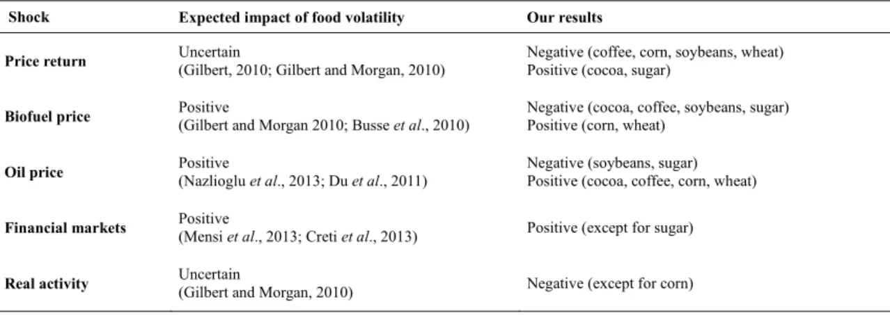
It is interesting to compare our results with previous ones available in the literature (see for instance Morgan, 2010). We note that, depending on the commodity, biofuels and oil price shocks have different impacts on volatility; financial market shocks drive food volatility higher, while real economic activity drives it lower (Table 4). Our findings are consistent with the previous results.
Table 4. Expected effects and results summary
Shock Expected impact of food volatility Our results
Price return Uncertain (Gilbert, 2010; Gilbert and Morgan, 2010) Negative (coffee, corn, soybeans, wheat) Positive (cocoa, sugar)
Biofuel price Positive
(Gilbert and Morgan 2010; Busse et al., 2010)
Negative (cocoa, coffee, soybeans, sugar) Positive (corn, wheat)
Oil price Positive
(Nazlioglu et al., 2013; Du et al., 2011)
Negative (soybeans, sugar) Positive (cocoa, coffee, corn, wheat)
Financial markets Positive
(Mensi et al., 2013; Creti et al., 2013) Positive (except for sugar)
Real activity Uncertain
(Gilbert and Morgan, 2010) Negative (except for corn) Source: Authors’ calculations.
13 Figure 4. Impulse response functions of food volatilities from the BVARs
Cocoa Coffee Corn Soybeans Sugar Wheat
Food Return Biofuels WTI Crude S&P 500 -0.7 -0.6 -0.5 -0.4 -0.3 -0.2 -0.10 0.1 0.2 0.3 0.4 1 3 5 7 9 11 13 15 17 19 21 23 -0.6 -0.5 -0.4 -0.3 -0.2 -0.1 0 0.1 0.2 0.3 1 3 5 7 9 11 13 15 17 19 21 23 -0.5 -0.4 -0.3 -0.2 -0.1 0 0.1 0.2 0.3 0.4 1 3 5 7 9 11 13 15 17 19 21 23 -0.7 -0.6 -0.5 -0.4 -0.3 -0.2 -0.1 0 0.1 0.2 1 3 5 7 9 11 13 15 17 19 21 23 -0.7 -0.6 -0.5 -0.4 -0.3 -0.2 -0.1 0 0.1 0.2 1 3 5 7 9 11 13 15 17 19 21 23 -0.3 -0.2 -0.1 0 0.1 0.2 0.3 0.4 0.5 1 3 5 7 9 11 13 15 17 19 21 23 -0.4 -0.3 -0.2 -0.1 0 0.1 0.2 0.3 1 3 5 7 9 11 13 15 17 19 21 23 -0.7 -0.6 -0.5 -0.4 -0.3 -0.2 -0.1 0 0.1 1 3 5 7 9 11 13 15 17 19 21 23 -0.3 -0.2 -0.1 0 0.1 0.2 0.3 0.4 1 3 5 7 9 11 13 15 17 19 21 23 -0.4 -0.3 -0.2 -0.1 0 0.1 0.2 1 3 5 7 9 11 13 15 17 19 21 23 -0.3 -0.25 -0.2 -0.15 -0.1 -0.05 0 0.05 0.1 0.15 0.2 1 3 5 7 9 11 13 15 17 19 21 23 -0.3 -0.2 -0.1 0 0.1 0.2 0.3 0.4 1 3 5 7 9 11 13 15 17 19 21 23 -0.5 -0.4 -0.3 -0.2 -0.10 0.1 0.2 0.3 0.4 0.5 0.6 1 3 5 7 9 11 13 15 17 19 21 23 -0.4 -0.3 -0.2 -0.1 0 0.1 0.2 0.3 0.4 0.5 1 3 5 7 9 11 13 15 17 19 21 23 -0.5 -0.4 -0.3 -0.2 -0.1 0 0.1 0.2 0.3 0.4 0.5 1 3 5 7 9 11 13 15 17 19 21 23 -0.5 -0.4 -0.3 -0.2 -0.1 0 0.1 0.2 0.3 1 3 5 7 9 11 13 15 17 19 21 23 -0.5 -0.4 -0.3 -0.2 -0.1 0 0.1 0.2 0.3 0.4 1 3 5 7 9 11 13 15 17 19 21 23 -0.3 -0.2 -0.10 0.1 0.2 0.3 0.4 0.5 0.6 0.7 1 3 5 7 9 11 13 15 17 19 21 23 -0.15 -0.1 -0.05 0 0.05 0.1 0.15 0.2 0.25 0.3 1 3 5 7 9 11 13 15 17 19 21 23 -0.2 -0.15 -0.1 -0.05 0 0.05 0.1 0.15 0.2 0.25 1 3 5 7 9 11 13 15 17 19 21 23 -0.2 -0.15 -0.1 -0.05 0 0.05 0.1 0.15 0.2 0.25 1 3 5 7 9 11 13 15 17 19 21 23 -0.15 -0.1 -0.05 0 0.05 0.1 0.15 0.2 0.25 1 3 5 7 9 11 13 15 17 19 21 23 -0.2 -0.15 -0.1 -0.05 0 0.05 0.1 0.15 0.2 1 3 5 7 9 11 13 15 17 19 21 23 -0.15 -0.1 -0.05 0 0.05 0.1 0.150.2 0.25 0.3 0.35 1 3 5 7 9 11 13 15 17 19 21 23
14
Cocoa Coffee Corn Soybeans Sugar Wheat
US IPI Food Volatility -50000 -40000 -30000 -20000 -10000 0 10000 20000 1 3 5 7 9 11131517192123 -30000 -20000 -10000 0 10000 20000 30000 1 3 5 7 9 11131517192123 -20000 -10000 0 10000 20000 30000 40000 50000 60000 1 3 5 7 9 11131517192123 -30000 -20000 -10000 0 10000 20000 30000 1 3 5 7 9 11131517192123 -30000 -20000 -10000 0 10000 20000 30000 40000 1 3 5 7 9 11131517192123 -30000 -25000 -20000 -15000 -10000 -5000 0 5000 10000 15000 1 3 5 7 9 11131517192123 0 0.2 0.4 0.6 0.8 1 1.2 1 3 5 7 9 11 13 15 17 19 21 23 -0.2 0 0.2 0.4 0.6 0.8 1 1.2 1 3 5 7 9 11 13 15 17 19 21 23 -0.2 0 0.2 0.4 0.6 0.8 1 1.2 1 3 5 7 9 11 13 15 17 19 21 23 -0.2 0 0.2 0.4 0.6 0.8 1 1.2 1 3 5 7 9 11 13 15 17 19 21 23 -0.2 0 0.2 0.4 0.6 0.8 1 1.2 1 3 5 7 9 11 13 15 17 19 21 23 -0.2 0 0.2 0.4 0.6 0.8 1 1.2 1 3 5 7 9 11 13 15 17 19 21 23
3.3. Robustness check
3.3.1. Introduction of alternative variables
In order to test the relevance of our specification, we run four additional models, introducing alternative measures for crude oil prices, financial markets indicators, real activity and volatility. First, we replace WTI crude oil prices with Brent crude oil prices. Second, we substitute the S&P 500 index with the MSCI World index and use global GDP instead of the US IPI. Lastly, we use IQR instead of standard deviation as a volatility measure.
Overall, the relationships remain steady, the parameters remain almost identical in the volatility equations (see Appendix 3) and the IRFs are very similar to the ones obtained in our benchmark model (see Appendices 4 to 6, 9A and 9B). However there is one notable exception, which is the response of volatility to a shock to the MSCI World index. Indeed, depending on the commodity, the volatility response to this shock is either negative or positive.
3.3.2. Testing for volatility spillovers
Here we test an alternative approach to look at the food price volatility by running a multivariate framework in which we only take into account the 6 different food volatilities. In this respect, our analysis goes beyond the classical approach adopted in recent studies. Indeed, the spillover analysis of food commodity price volatilities is based on a bivariate model in which each food commodity is exposed to stock market or crude oil volatility (Du et al, 2011, Nazlioglu et al., 2013, Mensi et al., 2013). We notice that:
Coffee and wheat volatilities are impacted most severely by a shock to cocoa volatility. The volatilities of corn and soybeans are driven upward, while the effect on sugar is ambiguous (see Appendices 7 and 8).
The volatility of commodities (except for soybeans and wheat) tends to increase after a shock to coffee volatility.
Cocoa and wheat volatilities decline following a corn volatility shock. Other commodities exhibit different reactions at different time horizons.
A soybean volatility shock generates a decline in volatility for cocoa and sugar. Coffee, corn and wheat react differently according to the time horizon.
The volatilities of cocoa and coffee display the strongest response to a sugar volatility shock. Grains (corn, soybeans and wheat) exhibit a very low response.
A wheat volatility shock implies decreasing volatility for corn, soybeans and sugar while the effects are fairly mixed for cocoa and coffee.
To sum up, we note that there are no clear uniform spillover effects between the food commodities under review. Hence, a multivariate framework with more information and diverse explanatory variables, similar to our benchmark framework, seems more coherent for modeling food price volatility.
3.3.3. What can we learn from the estimations of BVAR models based on the Normal-Wishart priors? In order to identify and assess the sensitivity of the empirical results to the choice of prior distributions, we estimate BVAR models based on Normal-Wishart prior distributions.
An analysis of the results leads to the following observations:
For most food commodities, the estimated coefficients based on both Minnesota and Normal-Wishart are generally of the same sign. They display similar values, albeit slightly lower in the case
16 of Normal-Wishart priors. For instance, for the coffee volatility equation, the Minnesota priors-based estimates of the coefficients of biofuels, the S&P 500 and the coffee volatility first lag are respectively 0.06, -0.09 and 0.89; in the case of the Normal-Wishart-based estimates, these coefficients are respectively 0.02, -0.09 and 0.57. These results can be extended for the other equations;
The analysis of IRFs stemming from the Normal-Wishart-based estimations shows that the impact of food volatility shocks is not significant (0 in all confidence intervals) in most cases. Nevertheless, the responses are qualitatively similar to those drawn from the Minnesota priors-based estimates, but of a lower magnitude.
Taking these points above into account, the Minnesota priors-based estimates allow us to draw clearer results. This seems to confirm the relevance of our choice of the Minnesota priors
4. Policy issues
4.1 What lesson can we draw from the literature?
Research papers have been more concerned by food price levels than volatilities. However, food price volatility has major consequences on both a macro and a micro level. Its impact is greater in the case of emerging economies, while developed economies are more concerned by oil price volatility. Food price volatility can affect the current account and nominal exchange rates. These effects are state-dependent and vary from one country to another. In 2011, China, the US, Brazil, India, Germany and France were major players in the global food trade in terms of absolute value. However, food trade was more important for countries such as Egypt or Senegal, where food imports accounted for more than 20% of total merchandise trade. This was also the case for Ivory Coast, Argentina or Uruguay where food exports accounted for more than 50% of total merchandise trade (see Table 2). The Food and Agriculture Organization (FAO) pointed out that for 14 countries, increases in the price of the more expensive cereal imports could widen the current account deficit by more than 2% of GDP (FAO, 2008). It is also important to note that food markets, food trade and dependencies varied over time (except in the case of small dependent countries such as Djibouti, Qatar, etc.), so many nations entered or left the FAO rankings.
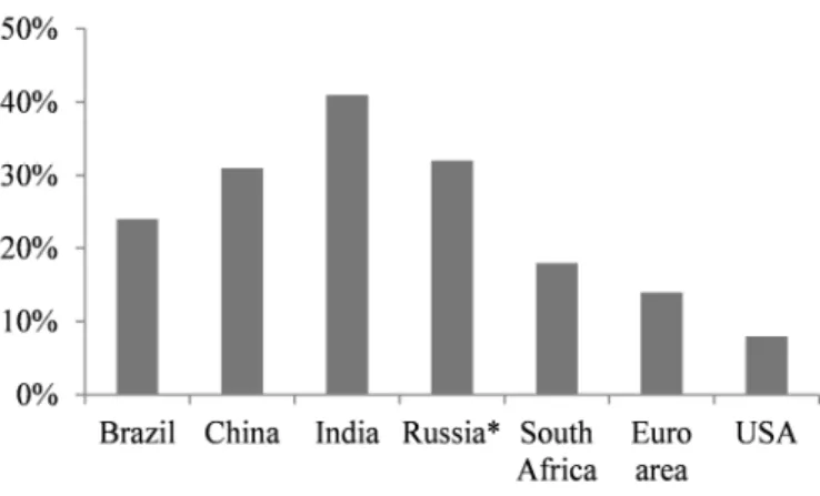
Food prices can also affect CPI, but this impact varies across countries. The weight of food in the CPI differs from one economy to another (see Figure 5), so clearly, the impact of changes in food prices or food volatility depends on the specific characteristics of the country. In the case of the BRICS, for example, the weight of food in the CPI ranges from around 18% for South Africa to 41% for India. In the euro area and the US, meanwhile, the weightings are 14% and 8% respectively. CPI and food prices increased in parallel in some countries during the huge expansion episode in 2007-2008 (FAO, 2008). Firms are also affected by food price volatility, through inflationary pressures caused by the wage-price spiral. As a consequence, national authorities sometimes need to implement costly stabilisation policies (e.g. food subsidies).
Figure 5. Food weights in CPIs
Source: OECD, *estimated.
Consumers in low income countries are the first to suffer from volatile and high food prices. Egypt, Haiti and Indonesia experienced “hunger riots” during the huge expansion episode of 2007-2008. From a global perspective, international institutions have to understand food price volatility in order to prevent and reduce it but also in order to take action against its undesired effects.
4.2 What lesson can we draw from the recent evolution of food price volatility?
In order to examine some policy issues, we estimate some BVAR models including the price volatility of staple foods (corn, soybeans and wheat), the industrial production index (IPI) and the consumer price index (CPI). The countries are selected on the basis of the availability of monthly indicators: the US, the euro area, Brazil, Russia and South Africa (see Appendix 10).
The results of the impulse response functions lead us to focus our analysis on IPI reactions to shocks in these countries (see Appendix 11a). Indeed, we obtain more meaningful results for the IPI. The main results of the analysis of these IRFs are:
- A corn volatility shock drives down the IPI for all countries except Brazil, the largest producer of ethanol. IPIs drop after 5 months for the US and the euro area and after 3 months for the other countries. The intensity and duration of the decrease is relatively low in all cases, with the exception of the US;
The reaction of the IPI following a soybean volatility shock is almost negligible for all countries, except for the US which displays a decrease during the first 5 months;
As for the other grains, a wheat volatility shock leads to a small decrease in the IPI for the euro area, Brazil, Russia and South Africa. The intensity of the decline is much greater for the US. We find that grain volatility shocks have a negative impact on IPIs for all countries, particularly in the US where the reaction is stronger. Volatility shocks can be interpreted as an increase in uncertainty. However, the decrease in the IPI means that suppliers protect themselves against the risk linked to large changes in the volatilities.
Finally, let us not forget that grain volatility shocks have no significant impact on CPIs in general (see Appendix 11b).
18
5. Conclusion
A Bayesian framework helps to show that the volatility of soft commodities is influenced by the price of the commodities themselves, by the US IPI, by biofuel and oil prices and by the price of financial assets. The US IPI has a negative impact on food price volatility, with the exception of soybeans. The impact of biofuel prices on corn and sugar volatilities is negative, while it is positive or zero in the case of other food commodities. Corn and wheat volatilities are negatively linked to crude oil prices, while, in the long run, coffee volatility is not correlated to oil prices. Financial market indicators, meanwhile, are strongly linked to food volatility. An analysis of impulse response functions yields the following conclusions:
A shock to price changes diminishes volatility for food commodities with the exception of corn and wheat;
Food volatility decreases after a biofuel price shock, except in the case of corn and wheat where it increases in the immediate aftermath of the shock then decreases over time;
Financial market shocks lead to higher volatilities;
Finally, a shock to the US IPI negatively impacts food price volatility except in the case of corn and sugar.
Regarding the IRF results, we observe that:
Cocoa and coffee show the same patterns regardless of the shock;
Soybeans, sugar and wheat display similar responses to the above except for one particular shock; The response to an oil shock differs in the case of soybeans;
The impact of US IPI shock is not the same for sugar nor is the biofuel price shock for wheat; Corn volatility displays quite different characteristics.
Robustness checks confirm the relevance of our benchmark model, since the results are broadly insensitive to the introduction of alternative variables. In addition, the tests for spillover effects show that a multivariate framework with alternative explanatory variables is more coherent for modelling food price volatility.
References
Abbot, P.C., C. Hurt and W.E. Tyner. (2008). What’s Driving Food Prices? Oak Brook, Illinois: Farm Foundation.
Alghalith, M. (2010). The Interaction Between Food Prices and Oil Prices. Energy Economics, 32(2), 1520-1522.
Banbura M., D. Giannone and L. Reichlin. (2010). Large Bayesian Vector Auto Regressions. Journal of Applied Econometrics, 25(1), 71-92.
Bloom, N. (2009). The Impact of Uncertainty Shocks. Econometrica, 77(3), 623-685.
Busse, S., B. Brummer and R. Ihle. (2010). Interdependencies Between Fossil Fuel and Renewable Energy Markets: The German Biodiesel Market. DARE Discussion Paper No. 1010.
Chakravorty, U., M. Hubert, M. Moreaux and L. Nøstbakken. (2010). Do Biofuel Mandates Raise Food Prices? IDEI, Working Paper No. 653.
Cooke, B. and M. Robles. (2009). Recent Food Price Movements: A Time Series Analysis. IFPRI Discussion Paper No. 00942.
Del Negro M. and F. Schorfheide . (2010). Bayesian Macroeconometrics. Prepared for Handbook of Bayesian Econometrics (mimeo).
Du, X., C.L. Yu and D.J. Hayes. (2011). Speculation and Volatility Spillover in the Crude Oil and Agricultural Commodity Markets: A Bayesian Analysis. Energy Economics, 33(3), 497-503. FAO. (2008). Soaring Food Prices: Facts, Perspectives, Impacts. Rome.
Fernandez-Villaverde, J., P.A. Guerron-Quitana, J. Rubio-Ramirez and M. Uribe. (2011b). Risk Matters: the Real Effects of Volatility Shocks. American Economic review, 101(6), 530-561. Fernandez-Villaverde, J., P.A. Guerron-Quitana, K. Kuester and J. Rubio-Ramirez. (2011a). Fiscal
Volatility Shocks and Economic Activity. NBER, Working Paper No. 17317.
Gilbert, C.L. (2010). How to Understand High Food Prices. Journal of Agricultural Economics, 61(2), 398-425.
Gilbert, C.L. and C.W. Morgan. (2010). Food Price Volatility. Philosophical Transactions of the Royal Society B-Biological Sciences, 365 (1554 ), 3023-3034.
Headey, D.D. (2011). Rethinking the Global Food Crisis: The Role of Trade Shocks. Food Policy, 36(2), 136-146.
Hernandez, A., M. Robles and M. Torero. (2011). Beyond the Numbers: How Urban Households in Central America Responded to the Recent Global Crises. IFPRI Issue Brief 67.
Kadiyala K.R. and S. Karlsson. (n.d.). Numerical Methods for Estimation and Inference in Bayesian VAR Models. Journal of Applied Econometrics, 12(2), 99-132.
Lemoine M. and C. Mougin. (2010). The Growth-Volatility Relationship: New Evidence Based on Stochastic Volatility in Means Models. Banque de France, Working Paper No. 382.
Litterman R.B. (1986). Forecasting with Bayesian Vector Autoregressions: Five Years of Experience. Journal of Business and Economic Statistics, 4(14), 25-38.
Martin, W. and K. Anderson. (2012). Export Restrictions and Price Insulation During Commodity Price Booms. American Journal of Agricultural Economics, 94(2), 422-427.
Mensi, W., M. Beljid, A. Boubaker and S. Managi. (2013). Correlations and Volatility Spillovers Across Commodity and Stock Markets: Linking Energies, Food, and Gold. Economic Modelling, 32, 15-22.
Mitchell, D. (2008). A Note on Rising Food Prices. Washington, DC: World Bank, Development Prospects Group, Policy Research Working Paper No. 4682.
Mumtaz H. and K. Theodoridis. (2012). The International Transmission of Volatility Shocks: An empirical Analysis. Bank of England, Working Paper No. 463.
20 Nazlioglu, S., C. Erdem and U. Soytas. (2013). Volatility Spillover between Oil and Agricultural
Commodity Markets. Energy Economics, 36, 658-665.
Piesse, J. and C. Thirtle. (2009). Three Bubbles and a Panic: An Explanatory Review of the Food Commodity Price Spikes of 2008. Food Policy, 34(2), 119-129.
Roache, S.K. (2010). What Explains the Rise in Food Price Volatility? IMF, Working Paper No. 10/129.
Robles, M., M. Torero and J.V. Braun. (2009). When Speculation Matters. IFPRI Issue Brief No. 57. Shi, S. and V. Arora. (2012). An Application of Models of Speculative Behaviour to Oil Prices.
Economics Letters, 115(3), 469-472.
Sims C.A. and T. Zha. (1998). Bayesian Methods For Dynamic Multivariate Models. International Economic review, 39(4), 949-1155.
Tadese, G., B. Algieri, M. Kalkuhl and J. von Braun. (2013). Drivers and Triggers of International Food Price Spikes and Volatility. Food Policy, In Press.
Timmer, C.P. (2010). Management of Rice Reserve Stocks in Asia: Analytical Issues and Country Experience. in: Commodity Market Review 2009-10, FAO, Rome, 87-120.
von Braun, J. (2011). Increasing and More Volatile Food Prices and the Consumer. in: Lusk, J. and Shogren, J. (Eds.), The Oxford Handbook of the Economics of Food Consumption and Policy, Oxford University Press, 612-628.
Wright, B. (2011). The Economics of Grain Price Volatility. Applied Economic Perspectives and Policy, 33(1), 32-58.
Appendix 1. Descriptive Statistics
BRENT COCOA COFFEE CORN GDP_WORLD IPI_US BIOFUELS
Mean 0.010 0.005 0.005 0.009 -0.013 0.001 0.008 Median 0.024 0.007 0.010 0.009 -0.051 0.001 0.005 Maximum 0.256 0.292 0.198 0.252 1.086 0.016 0.150 Minimum -0.444 -0.242 -0.278 -0.276 -1.013 -0.043 -0.192 Std. Dev. 0.100 0.083 0.091 0.095 0.311 0.008 0.065 Skewness -0.845 -0.078 -0.188 -0.474 0.432 -2.027 -0.306 Kurtosis 5.371 3.675 3.099 3.500 6.797 11.246 3.446 Jarque-Bera 51.580 2.918 0.917 6.980 92.229 513.563 3.492 Probability 0.000 0.233 0.632 0.031 0.000 0.000 0.174
MSCI_WORLD SOYBEANS SPX SUGAR WHEAT WTI
Mean 0.001 0.008 0.001 0.004 0.007 0.008 Median 0.007 0.019 0.008 0.000 0.010 0.019 Maximum 6.964 0.189 0.102 0.274 0.277 0.260 Minimum -6.972 -0.403 -0.186 -0.302 -0.363 -0.395 Std. Dev. 3.247 0.092 0.046 0.099 0.106 0.093 Skewness 0.005 -1.210 -0.782 -0.047 -0.528 -0.817 Kurtosis 4.561 5.986 4.293 3.223 4.246 5.185 Jarque-Bera 14.825 89.882 25.062 0.357 16.236 45.279 Probability 0.001 0.000 0.000 0.837 0.000 0.000
22
Appendix 2. Estimated parameters of the BVARs
Cocoa Return Biofuel WTI Crude S&P 500 US IPI Cocoa Volatility
Price Return-1 -0.158 -0.024 -0.013 -0.074 -0.002 0.039 (0.094) (0.074) (0.102) (0.05) (0.008) (0.031) [-0.277;-0.038] [-0.119;0.069] [-0.144;0.117] [-0.137;-0.01] [-0.012;0.008] [-0.001;0.078] Biofuel-1 -0.057 0.040 0.153 -0.074 0.002 0.021 (0.125) (0.098) (0.135) (0.066) (0.011) (0.04) [-0.217;0.104] [-0.087;0.165] [-0.022;0.325] [-0.157;0.009] [-0.012;0.015] [-0.03;0.071] WTI Crude-1 -0.008 -0.040 0.099 -0.001 0.001 0.011 (0.087) (0.068) (0.095) (0.047) (0.007) (0.028) [-0.119;0.102] [-0.128;0.047] [-0.023;0.222] [-0.062;0.06] [-0.009;0.01] [-0.026;0.047] S&P 500-1 -0.101 -0.025 0.419 0.207 0.004 -0.057 (0.177) (0.141) (0.195) (0.096) (0.015) (0.058) [-0.33;0.123] [-0.206;0.155] [0.167;0.67] [0.085;0.331] [-0.015;0.024] [-0.132;0.018] US IPI-1 0.666 1.201 1.754 1.365 0.112 0.038 (0.991) (0.785) (1.099) (0.536) (0.084) (0.323) [-0.589;1.946] [0.197;2.207] [0.328;3.166] [0.677;2.054] [0.004;0.219] [-0.378;0.447] Volatility-1 -0.043 -0.086 0.184 0.072 -0.010 0.801 (0.259) (0.204) (0.283) (0.14) (0.022) (0.085) [-0.375;0.291] [-0.344;0.179] [-0.186;0.547] [-0.107;0.252] [-0.038;0.018] [0.693;0.909] Price Return-2 -0.074 -0.003 0.083 -0.026 0.006 -0.019 (0.091) (0.073) (0.101) (0.049) (0.008) (0.03) [-0.191;0.042] [-0.096;0.091] [-0.046;0.213] [-0.089;0.038] [-0.004;0.016] [-0.057;0.02] Biofuel-2 0.041 0.047 0.065 0.046 -0.016 -0.022 (0.121) (0.095) (0.132) (0.065) (0.01) (0.039) [-0.114;0.194] [-0.076;0.169] [-0.103;0.236] [-0.037;0.129] [-0.029;-0.003] [-0.072;0.029] WTI Crude-2 -0.134 -0.005 -0.082 0.052 0.011 0.022 (0.081) (0.065) (0.089) (0.043) (0.007) (0.026) [-0.24;-0.03] [-0.089;0.077] [-0.195;0.032] [-0.003;0.107] [0.002;0.02] [-0.012;0.056] S&P 500-2 0.171 -0.059 0.105 -0.156 0.039 -0.043 (0.17) (0.135) (0.188) (0.092) (0.015) (0.056) [-0.049;0.386] [-0.234;0.116] [-0.133;0.347] [-0.274;-0.037] [0.021;0.058] [-0.115;0.029] US IPI-2 0.312 1.139 0.532 1.001 0.187 -0.477 (0.991) (0.794) (1.088) (0.538) (0.084) (0.328) [-0.979;1.589] [0.129;2.149] [-0.866;1.921] [0.318;1.701] [0.078;0.297] [-0.899;-0.056] Volatility-2 -0.315 0.029 -0.254 0.029 -0.021 0.019 (0.26) (0.21) (0.284) (0.142) (0.022) (0.085) [-0.647;0.02] [-0.239;0.3] [-0.614;0.113] [-0.151;0.212] [-0.05;0.007] [-0.089;0.128] Intercept 0.040 0.013 0.011 -0.009 0.003 0.016 (0.017) (0.014) (0.019) (0.009) (0.002) (0.006) [0.017;0.062] [-0.005;0.03] [-0.014;0.036] [-0.021;0.003] [0.001;0.005] [0.009;0.023] Source: Authors’ calculations; figures in parenthesis are standard deviations; figures in square brackets are the 10% and 90% centiles.
Coffee Return Biofuel WTI Crude S&P 500 US IPI Coffee Volatility Price Return-1 -0.166 -0.077 -0.032 -0.038 -0.001 -0.006 (0.086) (0.067) (0.092) (0.045) (0.007) (0.033) [-0.275;-0.056] [-0.163;0.008] [-0.149;0.085] [-0.095;0.02] [-0.01;0.009] [-0.048;0.037] Biofuel-1 0.104 0.024 0.163 -0.091 0.003 0.056 (0.128) (0.099) (0.137) (0.067) (0.011) (0.049) [-0.06;0.27] [-0.104;0.15] [-0.015;0.336] [-0.175;-0.005] [-0.011;0.016] [-0.006;0.118] WTI Crude-1 -0.065 -0.035 0.100 -0.014 0.001 0.026 (0.087) (0.067) (0.094) (0.046) (0.007) (0.033) [-0.176;0.045] [-0.122;0.052] [-0.02;0.222] [-0.074;0.045] [-0.008;0.01] [-0.017;0.069] S&P 500-1 0.053 0.000 0.414 0.253 0.000 -0.093 (0.182) (0.142) (0.196) (0.097) (0.015) (0.071) [-0.182;0.283] [-0.18;0.183] [0.159;0.667] [0.13;0.377] [-0.019;0.02] [-0.184;-0.002] US IPI-1 1.464 1.173 1.929 1.382 0.152 -0.013 (0.993) (0.772) (1.08) (0.527) (0.083) (0.382) [0.206;2.761] [0.179;2.158] [0.55;3.325] [0.704;2.054] [0.045;0.258] [-0.507;0.477] Volatility-1 -0.238 -0.395 0.138 -0.002 0.001 0.893 (0.217) (0.168) (0.233) (0.115) (0.018) (0.084) [-0.516;0.042] [-0.607;-0.177] [-0.162;0.435] [-0.149;0.147] [-0.022;0.025] [0.786;1] Price Return-2 0.074 0.104 -0.009 0.027 0.001 -0.092 (0.084) (0.067) (0.091) (0.044) (0.007) (0.033) [-0.034;0.181] [0.019;0.189] [-0.126;0.109] [-0.03;0.084] [-0.008;0.011] [-0.134;-0.049] Biofuel-2 -0.034 0.013 0.105 0.042 -0.013 0.003 (0.124) (0.096) (0.133) (0.066) (0.01) (0.047) [-0.193;0.124] [-0.111;0.135] [-0.065;0.275] [-0.043;0.127] [-0.026;0] [-0.057;0.064] WTI Crude-2 0.059 -0.014 -0.070 0.046 0.012 -0.028 (0.082) (0.064) (0.088) (0.043) (0.007) (0.032) [-0.047;0.165] [-0.096;0.069] [-0.182;0.044] [-0.009;0.101] [0.003;0.021] [-0.069;0.012] S&P 500-2 -0.035 -0.142 0.092 -0.160 0.037 0.063 (0.176) (0.137) (0.19) (0.093) (0.015) (0.068) [-0.261;0.188] [-0.316;0.032] [-0.149;0.335] [-0.28;-0.041] [0.018;0.055] [-0.023;0.15] US IPI-2 0.774 0.935 0.593 0.829 0.213 -0.559 (0.993) (0.783) (1.078) (0.531) (0.084) (0.389) [-0.503;2.04] [-0.069;1.936] [-0.792;1.993] [0.152;1.514] [0.105;0.32] [-1.056;-0.057] Volatility-2 0.217 0.148 -0.128 0.036 -0.009 -0.148 (0.216) (0.171) (0.232) (0.116) (0.018) (0.084) [-0.059;0.491] [-0.07;0.369] [-0.421;0.17] [-0.11;0.185] [-0.032;0.015] [-0.255;-0.04] Intercept 0.005 0.030 0.003 -0.003 0.001 0.023 (0.016) (0.012) (0.017) (0.008) (0.001) (0.006) [-0.016;0.025] [0.014;0.045] [-0.019;0.025] [-0.014;0.008] [-0.001;0.003] [0.015;0.031] Source: Authors’ calculations; figures in parenthesis are standard deviations; figures in square brackets are the 10% and 90% centiles.
24 Corn Return Biofuel WTI Crude S&P 500 US IPI Corn Volatility
Price Return-1 -0.129 0.002 -0.098 -0.061 -0.006 0.044 (0.132) (0.091) (0.125) (0.061) (0.01) (0.045) [-0.296;0.04] [-0.114;0.117] [-0.259;0.061] [-0.139;0.016] [-0.019;0.006] [-0.014;0.102] Biofuel-1 0.113 0.027 0.234 -0.054 0.012 -0.008 (0.193) (0.133) (0.183) (0.089) (0.014) (0.065) [-0.135;0.362] [-0.144;0.194] [-0.003;0.467] [-0.167;0.06] [-0.007;0.03] [-0.091;0.074] WTI Crude-1 -0.135 -0.040 0.100 -0.016 0.001 -0.004 (0.097) (0.067) (0.094) (0.046) (0.007) (0.033) [-0.259;-0.012] [-0.126;0.045] [-0.021;0.221] [-0.075;0.044] [-0.008;0.01] [-0.046;0.039] S&P 500-1 0.169 -0.015 0.443 0.257 0.000 0.055 (0.2) (0.14) (0.193) (0.095) (0.015) (0.069) [-0.091;0.423] [-0.192;0.166] [0.193;0.692] [0.136;0.38] [-0.019;0.02] [-0.034;0.144] US IPI-1 2.017 1.285 1.893 1.333 0.181 0.012 (1.124) (0.778) (1.089) (0.532) (0.083) (0.384) [0.593;3.48] [0.292;2.288] [0.498;3.296] [0.651;2.013] [0.073;0.287] [-0.483;0.5] Volatility-1 -0.103 -0.004 -0.128 0.004 0.031 0.898 (0.251) (0.173) (0.241) (0.119) (0.019) (0.086) [-0.425;0.218] [-0.223;0.22] [-0.44;0.182] [-0.148;0.158] [0.007;0.055] [0.787;1.008] Price Return-2 0.112 0.084 0.223 0.042 0.002 -0.046 (0.122) (0.086) (0.119) (0.058) (0.009) (0.042) [-0.045;0.268] [-0.025;0.193] [0.072;0.374] [-0.033;0.117] [-0.01;0.014] [-0.099;0.009] Biofuel-2 0.146 -0.028 -0.100 0.003 -0.014 -0.067 (0.177) (0.124) (0.171) (0.084) (0.013) (0.061) [-0.078;0.371] [-0.189;0.13] [-0.32;0.117] [-0.104;0.11] [-0.031;0.003] [-0.146;0.01] WTI Crude-2 -0.114 -0.002 -0.074 0.046 0.013 -0.035 (0.092) (0.065) (0.089) (0.043) (0.007) (0.032) [-0.234;0.004] [-0.086;0.082] [-0.187;0.04] [-0.01;0.102] [0.004;0.021] [-0.076;0.006] S&P 500-2 -0.203 -0.077 0.042 -0.153 0.034 -0.019 (0.198) (0.137) (0.19) (0.093) (0.015) (0.068) [-0.454;0.048] [-0.25;0.097] [-0.202;0.285] [-0.274;-0.034] [0.015;0.053] [-0.105;0.069] US IPI-2 1.720 1.186 0.523 0.854 0.223 -0.161 (1.105) (0.777) (1.068) (0.528) (0.083) (0.386) [0.291;3.136] [0.19;2.177] [-0.85;1.913] [0.181;1.532] [0.116;0.329] [-0.659;0.337] Volatility-2 0.099 0.110 0.141 0.032 -0.021 -0.195 (0.247) (0.175) (0.235) (0.118) (0.019) (0.085) [-0.219;0.415] [-0.111;0.333] [-0.157;0.448] [-0.12;0.184] [-0.044;0.003] [-0.302;-0.085] Intercept 0.008 -0.003 0.003 -0.003 -0.001 0.030 (0.019) (0.013) (0.018) (0.009) (0.001) (0.007) [-0.016;0.033] [-0.02;0.013] [-0.021;0.026] [-0.015;0.008] [-0.003;0.001] [0.021;0.038] Source: Authors’ calculations; figures in parenthesis are standard deviations; figures in square brackets are the 10% and 90% centiles.
Soybeans Return Biofuel WTI Crude S&P 500 US IPI Soybeans Volatility Price Return-1 -0.221 -0.142 0.132 0.002 -0.011 0.034 (0.161) (0.114) (0.158) (0.077) (0.012) (0.059) [-0.424;-0.014] [-0.286;0.002] [-0.071;0.334] [-0.096;0.1] [-0.027;0.005] [-0.041;0.109] Biofuel-1 0.164 0.197 -0.031 -0.121 0.016 -0.029 (0.227) (0.161) (0.221) (0.108) (0.017) (0.081) [-0.129;0.459] [-0.009;0.402] [-0.316;0.249] [-0.257;0.017] [-0.006;0.038] [-0.133;0.074] WTI Crude-1 -0.097 -0.077 0.113 -0.012 -0.001 0.031 (0.097) (0.069) (0.096) (0.047) (0.007) (0.035) [-0.221;0.025] [-0.166;0.011] [-0.011;0.236] [-0.073;0.049] [-0.01;0.009] [-0.014;0.077] S&P 500-1 0.283 0.012 0.394 0.235 0.000 -0.052 (0.195) (0.14) (0.194) (0.095) (0.015) (0.072) [0.032;0.53] [-0.166;0.194] [0.143;0.646] [0.114;0.359] [-0.019;0.019] [-0.144;0.039] US IPI-1 1.483 1.397 1.778 1.288 0.158 -0.739 (1.07) (0.762) (1.067) (0.521) (0.082) (0.389) [0.117;2.871] [0.421;2.375] [0.417;3.148] [0.622;1.954] [0.052;0.262] [-1.238;-0.246] Volatility-1 -0.244 -0.101 -0.085 0.031 0.000 0.876 (0.252) (0.18) (0.25) (0.122) (0.019) (0.092) [-0.57;0.082] [-0.327;0.131] [-0.408;0.235] [-0.128;0.188] [-0.025;0.025] [0.757;0.994] Price Return-2 0.275 0.106 -0.078 -0.045 0.001 -0.074 (0.137) (0.1) (0.137) (0.067) (0.011) (0.05) [0.099;0.449] [-0.02;0.233] [-0.251;0.098] [-0.131;0.042] [-0.012;0.015] [-0.138;-0.01] Biofuel-2 -0.185 -0.091 0.199 0.092 -0.014 0.024 (0.193) (0.139) (0.192) (0.094) (0.015) (0.071) [-0.429;0.062] [-0.273;0.087] [-0.045;0.444] [-0.029;0.213] [-0.033;0.005] [-0.067;0.114] WTI Crude-2 -0.003 0.009 -0.077 0.044 0.012 0.061 (0.091) (0.065) (0.09) (0.044) (0.007) (0.033) [-0.119;0.112] [-0.074;0.092] [-0.19;0.039] [-0.012;0.1] [0.004;0.021] [0.019;0.104] S&P 500-2 -0.125 -0.022 0.079 -0.141 0.040 0.029 (0.193) (0.137) (0.19) (0.094) (0.015) (0.07) [-0.371;0.123] [-0.195;0.155] [-0.163;0.322] [-0.263;-0.021] [0.021;0.059] [-0.06;0.12] US IPI-2 0.439 1.013 0.644 0.879 0.216 0.278 (1.087) (0.785) (1.084) (0.533) (0.084) (0.402) [-0.951;1.832] [-0.004;2.02] [-0.755;2.043] [0.2;1.568] [0.109;0.323] [-0.239;0.796] Volatility-2 0.055 -0.069 -0.092 -0.021 -0.002 -0.162 (0.239) (0.175) (0.235) (0.118) (0.019) (0.088) [-0.255;0.361] [-0.292;0.157] [-0.393;0.212] [-0.172;0.132] [-0.026;0.021] [-0.274;-0.05] Intercept 0.025 0.022 0.020 -0.001 0.001 0.025 (0.017) (0.012) (0.017) (0.008) (0.001) (0.006) [0.003;0.047] [0.007;0.038] [-0.002;0.042] [-0.011;0.01] [-0.001;0.002] [0.017;0.033] Source: Authors’ calculations; figures in parenthesis are standard deviations; figures in square brackets are the 10% and 90% centiles.
26 Sugar Return Biofuel WTI Crude S&P 500 US IPI Sugar Volatility
Price Return-1 0.132 0.043 -0.051 0.016 -0.002 0.011 (0.093) (0.062) (0.086) (0.042) (0.007) (0.035) [0.015;0.252] [-0.037;0.122] [-0.162;0.058] [-0.037;0.069] [-0.01;0.007] [-0.034;0.056] Biofuel-1 0.275 0.015 0.172 -0.128 0.005 -0.024 (0.149) (0.099) (0.136) (0.066) (0.011) (0.055) [0.083;0.468] [-0.113;0.14] [-0.004;0.347] [-0.212;-0.044] [-0.009;0.019] [-0.093;0.046] WTI Crude-1 -0.140 -0.057 0.079 -0.025 0.000 0.021 (0.102) (0.068) (0.095) (0.046) (0.007) (0.038) [-0.27;-0.013] [-0.144;0.03] [-0.042;0.201] [-0.085;0.035] [-0.009;0.009] [-0.028;0.07] S&P 500-1 -0.164 -0.026 0.354 0.234 -0.001 -0.054 (0.207) (0.139) (0.193) (0.096) (0.015) (0.078) [-0.433;0.098] [-0.204;0.152] [0.106;0.605] [0.113;0.357] [-0.02;0.019] [-0.155;0.046] US IPI-1 -0.305 1.237 1.942 1.316 0.147 -0.221 (1.149) (0.767) (1.074) (0.525) (0.082) (0.429) [-1.768;1.187] [0.259;2.219] [0.573;3.316] [0.65;1.987] [0.041;0.252] [-0.774;0.325] Volatility-1 -0.345 -0.050 0.052 0.031 0.012 0.830 (0.221) (0.147) (0.204) (0.101) (0.016) (0.083) [-0.627;-0.061] [-0.238;0.141] [-0.211;0.315] [-0.097;0.162] [-0.008;0.032] [0.723;0.935] Price Return-2 -0.124 -0.071 0.050 0.030 -0.004 0.012 (0.089) (0.06) (0.083) (0.041) (0.007) (0.034) [-0.239;-0.012] [-0.149;0.006] [-0.056;0.157] [-0.023;0.082] [-0.013;0.004] [-0.031;0.055] Biofuel-2 -0.074 0.078 0.100 0.023 -0.008 -0.153 (0.146) (0.098) (0.135) (0.066) (0.01) (0.055) [-0.261;0.113] [-0.048;0.202] [-0.074;0.273] [-0.064;0.108] [-0.021;0.006] [-0.223;-0.083] WTI Crude-2 0.125 0.002 -0.092 0.043 0.012 0.010 (0.096) (0.065) (0.089) (0.043) (0.007) (0.036) [0;0.248] [-0.082;0.084] [-0.205;0.022] [-0.013;0.098] [0.003;0.021] [-0.037;0.056] S&P 500-2 0.080 -0.073 0.072 -0.143 0.036 0.146 (0.202) (0.135) (0.188) (0.092) (0.015) (0.076) [-0.179;0.335] [-0.247;0.102] [-0.168;0.315] [-0.261;-0.025] [0.017;0.055] [0.05;0.245] US IPI-2 0.083 1.327 0.761 0.926 0.228 -0.053 (1.147) (0.78) (1.075) (0.53) (0.083) (0.439) [-1.389;1.543] [0.323;2.324] [-0.623;2.161] [0.251;1.606] [0.12;0.335] [-0.615;0.516] Volatility-2 0.148 -0.044 -0.296 -0.114 -0.014 -0.028 (0.218) (0.149) (0.201) (0.1) (0.016) (0.082) [-0.129;0.428] [-0.235;0.148] [-0.548;-0.037] [-0.241;0.016] [-0.034;0.007] [-0.132;0.079] Intercept 0.023 0.016 0.028 0.008 0.000 0.021 (0.016) (0.011) (0.015) (0.007) (0.001) (0.006) [0.003;0.044] [0.003;0.03] [0.009;0.047] [-0.001;0.018] [-0.001;0.002] [0.013;0.029] Source: Authors’ calculations; figures in parenthesis are standard deviations; figures in square brackets are the 10% and 90% centiles.
Wheat Return Biofuel WTI Crude S&P 500 US IPI Wheat Volatility Price Return-1 0.006 0.033 -0.068 0.020 -0.003 -0.035 (0.099) (0.061) (0.084) (0.041) (0.007) (0.036) [-0.119;0.133] [-0.046;0.111] [-0.176;0.04] [-0.032;0.073] [-0.011;0.005] [-0.08;0.011] Biofuel-1 -0.061 0.007 0.206 -0.136 0.005 0.052 (0.17) (0.104) (0.144) (0.07) (0.011) (0.06) [-0.279;0.16] [-0.127;0.139] [0.019;0.389] [-0.225;-0.046] [-0.009;0.02] [-0.024;0.127] WTI Crude-1 -0.091 -0.045 0.070 -0.019 0.002 -0.053 (0.111) (0.068) (0.095) (0.047) (0.007) (0.04) [-0.232;0.048] [-0.133;0.042] [-0.052;0.193] [-0.079;0.042] [-0.007;0.012] [-0.104;-0.002] S&P 500-1 -0.290 -0.022 0.421 0.246 -0.001 0.007 (0.223) (0.139) (0.192) (0.095) (0.015) (0.081) [-0.579;-0.009] [-0.199;0.157] [0.173;0.669] [0.125;0.369] [-0.02;0.018] [-0.097;0.111] US IPI-1 1.625 1.231 1.823 1.273 0.152 0.314 (1.245) (0.77) (1.078) (0.526) (0.082) (0.446) [0.04;3.249] [0.239;2.216] [0.441;3.212] [0.596;1.946] [0.044;0.257] [-0.263;0.887] Volatility-1 0.073 0.121 0.310 0.170 -0.009 0.737 (0.236) (0.145) (0.202) (0.1) (0.016) (0.085) [-0.228;0.375] [-0.063;0.31] [0.05;0.568] [0.042;0.298] [-0.029;0.011] [0.629;0.845] Price Return-2 0.045 0.025 -0.027 0.050 0.003 -0.102 (0.095) (0.059) (0.082) (0.04) (0.006) (0.034) [-0.076;0.167] [-0.051;0.101] [-0.132;0.078] [-0.001;0.102] [-0.005;0.012] [-0.146;-0.058] Biofuel-2 -0.102 0.031 0.134 0.003 -0.014 0.085 (0.165) (0.102) (0.142) (0.069) (0.011) (0.059) [-0.312;0.111] [-0.1;0.162] [-0.047;0.314] [-0.087;0.092] [-0.028;0] [0.01;0.161] WTI Crude-2 -0.053 0.011 -0.056 0.068 0.013 -0.065 (0.105) (0.066) (0.09) (0.044) (0.007) (0.038) [-0.189;0.081] [-0.074;0.095] [-0.171;0.06] [0.011;0.124] [0.004;0.021] [-0.114;-0.017] S&P 500-2 -0.169 -0.050 0.079 -0.147 0.035 0.008 (0.218) (0.135) (0.188) (0.092) (0.015) (0.079) [-0.452;0.108] [-0.223;0.122] [-0.161;0.322] [-0.265;-0.029] [0.017;0.054] [-0.092;0.109] US IPI-2 2.599 1.116 0.650 0.768 0.214 -0.496 (1.237) (0.776) (1.067) (0.527) (0.083) (0.451) [1.01;4.175] [0.124;2.104] [-0.713;2.039] [0.097;1.449] [0.107;0.32] [-1.075;0.087] Volatility-2 0.043 -0.132 -0.231 -0.155 -0.003 0.052 (0.234) (0.148) (0.2) (0.1) (0.016) (0.085) [-0.257;0.342] [-0.321;0.058] [-0.484;0.027] [-0.282;-0.026] [-0.023;0.017] [-0.055;0.162] Intercept -0.004 0.008 -0.004 -0.002 0.002 0.023 (0.019) (0.012) (0.017) (0.008) (0.001) (0.007) [-0.028;0.021] [-0.007;0.023] [-0.025;0.018] [-0.012;0.009] [0;0.003] [0.014;0.032] Source: Authors’ calculations; figures in parenthesis are standard deviations; figures in square brackets are the 10% and 90% centiles.
28
Appendix 3. Comparison of volatility equations
Cocoa
Baseline with Brent with MSCI with GDP World with IQR
Price Return-1 0.039 0.036 0.042 0.021 (0.031) (0.031) (0.031) (0.018) [-0.001;0.078] [-0.004;0.076] [0.003;0.082] [-0.002;0.045] Biofuel-1 0.021 0.018 0.008 -0.030 (0.04) (0.04) (0.038) (0.024) [-0.03;0.071] [-0.033;0.068] [-0.04;0.056] [-0.061;0] Oil Price-1 0.011 0.018 0.002 0.013 (0.028) (0.027) (0.027) (0.017) [-0.026;0.047] [-0.016;0.052] [-0.034;0.037] [-0.009;0.034] FINANCIAL MKT.-1 -0.057 -0.057 0.000 0.001 (0.058) (0.057) (0.001) (0.035) [-0.132;0.018] [-0.13;0.017] [-0.001;0.001] [-0.044;0.046] REAL ACTIVITY-1 0.038 0.049 0.034 -0.236 (0.323) (0.324) (0.324) (0.191) [-0.378;0.447] [-0.366;0.46] [-0.381;0.445] [-0.48;0.006] Volatility-1 0.801 0.801 0.803 0.749 (0.085) (0.085) (0.085) (0.08) [0.693;0.909] [0.693;0.908] [0.696;0.911] [0.648;0.851] Price Return-2 -0.019 -0.016 -0.014 0.046 (0.03) (0.03) (0.03) (0.018) [-0.057;0.02] [-0.055;0.022] [-0.052;0.025] [0.023;0.069] Biofuel-2 -0.022 -0.022 -0.026 -0.048 (0.039) (0.04) (0.038) (0.023) [-0.072;0.029] [-0.072;0.03] [-0.074;0.022] [-0.078;-0.018] Oil Price-2 0.022 0.003 0.016 -0.016 (0.026) (0.024) (0.026) (0.016) [-0.012;0.056] [-0.028;0.033] [-0.018;0.049] [-0.036;0.004] FINANCIAL MKT.-2 -0.043 -0.040 0.000 -0.018 (0.056) (0.056) (0.001) (0.033) [-0.115;0.029] [-0.112;0.033] [-0.001;0.001] [-0.061;0.024] REAL ACTIVITY-2 -0.477 -0.452 -0.544 -0.206 (0.328) (0.327) (0.322) (0.196) [-0.899;-0.056] [-0.875;-0.033] [-0.963;-0.131] [-0.457;0.045] Volatility-2 0.019 0.019 0.010 0.074 (0.085) (0.085) (0.085) (0.078) [-0.089;0.128] [-0.089;0.129] [-0.098;0.12] [-0.024;0.173] Intercept 0.016 0.016 0.017 0.014 (0.006) (0.006) (0.006) (0.004) [0.009;0.023] [0.009;0.023] [0.01;0.024] [0.009;0.02] Source: Authors’ calculations; figures in parenthesis are standard deviations; figures in square brackets are the 10% and 90% centiles.
Coffee
Baseline with Brent with MSCI with GDP World with IQR
Price Return-1 -0.006 -0.003 -0.015 0.016 (0.033) (0.034) (0.033) (0.017) [-0.048;0.037] [-0.046;0.04] [-0.057;0.027] [-0.005;0.038] Biofuel-1 0.056 0.064 0.044 0.013 (0.049) (0.049) (0.048) (0.024) [-0.006;0.118] [0.001;0.125] [-0.018;0.104] [-0.017;0.043] Oil Price-1 0.026 0.002 0.021 0.020 (0.033) (0.032) (0.033) (0.017) [-0.017;0.069] [-0.038;0.043] [-0.021;0.063] [-0.002;0.041] FINANCIAL MKT.-1 -0.093 -0.084 0.000 -0.072 (0.071) (0.07) (0.001) (0.035) [-0.184;-0.002] [-0.174;0.005] [-0.002;0.001] [-0.117;-0.027] REAL ACTIVITY-1 -0.013 -0.018 0.010 -0.224 (0.382) (0.383) (0.383) (0.191) [-0.507;0.477] [-0.514;0.474] [-0.483;0.5] [-0.471;0.022] Volatility-1 0.893 0.891 0.897 0.982 (0.084) (0.084) (0.083) (0.081) [0.786;1] [0.784;0.998] [0.791;1.003] [0.878;1.085] Price Return-2 -0.092 -0.091 -0.087 -0.014 (0.033) (0.033) (0.032) (0.017) [-0.134;-0.049] [-0.134;-0.049] [-0.128;-0.045] [-0.035;0.007] Biofuel-2 0.003 0.002 0.017 -0.020 (0.047) (0.048) (0.047) (0.023) [-0.057;0.064] [-0.059;0.063] [-0.042;0.077] [-0.049;0.01] Oil Price-2 -0.028 -0.004 -0.022 0.007 (0.032) (0.029) (0.031) (0.016) [-0.069;0.012] [-0.041;0.033] [-0.062;0.018] [-0.014;0.027] FINANCIAL MKT.-2 0.063 0.059 0.000 0.021 (0.068) (0.068) (0.001) (0.034) [-0.023;0.15] [-0.028;0.148] [-0.001;0.002] [-0.023;0.065] REAL ACTIVITY-2 -0.559 -0.566 -0.646 -0.212 (0.389) (0.388) (0.383) (0.195) [-1.056;-0.057] [-1.063;-0.067] [-1.14;-0.152] [-0.463;0.04] Volatility-2 -0.148 -0.144 -0.156 -0.193 (0.084) (0.084) (0.083) (0.08) [-0.255;-0.04] [-0.25;-0.036] [-0.261;-0.049] [-0.294;-0.09] Intercept 0.023 0.023 0.024 0.018 (0.006) (0.006) (0.006) (0.005) [0.015;0.031] [0.015;0.031] [0.016;0.032] [0.012;0.024] Source: Authors’ calculations; figures in parenthesis are standard deviations; figures in square brackets are the 10% and 90% centiles.
30
Corn
Baseline with Brent with MSCI with GDP World with IQR
Price Return-1 0.044 0.048 0.047 0.049 (0.045) (0.045) (0.045) (0.027) [-0.014;0.102] [-0.01;0.106] [-0.011;0.104] [0.014;0.083] Biofuel-1 -0.008 -0.008 -0.002 -0.048 (0.065) (0.065) (0.064) (0.038) [-0.091;0.074] [-0.092;0.075] [-0.085;0.079] [-0.097;0] Oil Price-1 -0.004 -0.012 0.003 -0.005 (0.033) (0.031) (0.032) (0.02) [-0.046;0.039] [-0.052;0.028] [-0.039;0.044] [-0.03;0.02] FINANCIAL MKT.-1 0.055 0.057 0.001 -0.035 (0.069) (0.068) (0.001) (0.041) [-0.034;0.144] [-0.032;0.144] [-0.001;0.002] [-0.087;0.018] REAL ACTIVITY-1 0.012 -0.006 -0.009 0.023 (0.384) (0.385) (0.385) (0.222) [-0.483;0.5] [-0.503;0.483] [-0.504;0.481] [-0.264;0.307] Volatility-1 0.898 0.904 0.895 1.044 (0.086) (0.087) (0.086) (0.086) [0.787;1.008] [0.792;1.015] [0.786;1.004] [0.933;1.154] Price Return-2 -0.046 -0.044 -0.051 -0.022 (0.042) (0.042) (0.042) (0.025) [-0.099;0.009] [-0.098;0.011] [-0.104;0.003] [-0.054;0.01] Biofuel-2 -0.067 -0.073 -0.073 -0.013 (0.061) (0.061) (0.061) (0.036) [-0.146;0.01] [-0.153;0.005] [-0.152;0.003] [-0.06;0.032] Oil Price-2 -0.035 -0.006 -0.036 -0.016 (0.032) (0.029) (0.032) (0.019) [-0.076;0.006] [-0.043;0.031] [-0.076;0.005] [-0.04;0.008] FINANCIAL MKT.-2 -0.019 -0.029 0.001 0.057 (0.068) (0.068) (0.001) (0.04) [-0.105;0.069] [-0.115;0.06] [-0.001;0.002] [0.007;0.109] REAL ACTIVITY-2 -0.161 -0.193 -0.098 -0.307 (0.386) (0.385) (0.381) (0.227) [-0.659;0.337] [-0.688;0.304] [-0.59;0.389] [-0.598;-0.015] Volatility-2 -0.195 -0.197 -0.193 -0.258 (0.085) (0.085) (0.085) (0.084) [-0.302;-0.085] [-0.304;-0.087] [-0.3;-0.084] [-0.364;-0.149] Intercept 0.030 0.029 0.030 0.019 (0.007) (0.007) (0.007) (0.005) [0.021;0.038] [0.021;0.038] [0.021;0.038] [0.013;0.025] Source: Authors’ calculations; figures in parenthesis are standard deviations; figures in square brackets are the 10% and 90% centiles.
Soybeans
Baseline with Brent with MSCI with GDP World with IQR
Price Return-1 0.034 0.032 0.027 0.029 (0.059) (0.059) (0.058) (0.035) [-0.041;0.109] [-0.043;0.107] [-0.046;0.101] [-0.016;0.073] Biofuel-1 -0.029 -0.023 -0.027 -0.021 (0.081) (0.081) (0.081) (0.048) [-0.133;0.074] [-0.127;0.08] [-0.13;0.075] [-0.082;0.039] Oil Price-1 0.031 0.021 0.023 -0.002 (0.035) (0.033) (0.034) (0.021) [-0.014;0.077] [-0.021;0.063] [-0.021;0.067] [-0.029;0.026] FINANCIAL MKT.-1 -0.052 -0.047 0.000 -0.028 (0.072) (0.071) (0.001) (0.043) [-0.144;0.039] [-0.138;0.043] [-0.002;0.001] [-0.083;0.028] REAL ACTIVITY-1 -0.739 -0.779 -0.763 -0.270 (0.389) (0.39) (0.39) (0.238) [-1.238;-0.246] [-1.279;-0.285] [-1.263;-0.269] [-0.579;0.035] Volatility-1 0.876 0.877 0.871 0.882 (0.092) (0.092) (0.093) (0.092) [0.757;0.994] [0.758;0.995] [0.753;0.989] [0.763;1] Price Return-2 -0.074 -0.072 -0.068 -0.038 (0.05) (0.051) (0.05) (0.03) [-0.138;-0.01] [-0.136;-0.007] [-0.132;-0.004] [-0.077;0.001] Biofuel-2 0.024 0.016 0.023 0.038 (0.071) (0.071) (0.071) (0.043) [-0.067;0.114] [-0.075;0.105] [-0.068;0.113] [-0.017;0.092] Oil Price-2 0.061 0.072 0.069 0.010 (0.033) (0.03) (0.033) (0.02) [0.019;0.104] [0.034;0.11] [0.027;0.111] [-0.016;0.035] FINANCIAL MKT.-2 0.029 0.035 0.001 0.022 (0.07) (0.071) (0.001) (0.042) [-0.06;0.12] [-0.054;0.126] [-0.001;0.002] [-0.032;0.076] REAL ACTIVITY-2 0.278 0.284 0.252 -0.062 (0.402) (0.401) (0.396) (0.242) [-0.239;0.796] [-0.233;0.801] [-0.259;0.764] [-0.375;0.252] Volatility-2 -0.162 -0.159 -0.160 -0.020 (0.088) (0.088) (0.089) (0.089) [-0.274;-0.05] [-0.271;-0.047] [-0.275;-0.045] [-0.131;0.095] Intercept 0.025 0.024 0.025 0.012 (0.006) (0.006) (0.006) (0.004) [0.017;0.033] [0.016;0.033] [0.017;0.033] [0.006;0.017] Source: Authors’ calculations; figures in parenthesis are standard deviations; figures in square brackets are the 10% and 90% centiles.