Fisheries management and intergenerational equity
Ivar Ekeland, Claudio Pareja, U. Rashid Sumaila
Fisheries management and intergenerational equity
Ivar Ekeland, Canada Research Chair in Mathematical Economics, UBC
Claudio Pareja, Departamento de Ingenier´ıa Matem´atica, Universidad de Chile
U. Rashid Sumaila
∗, Fisheries Centre, UBC
January 25, 2009
Abstract
We adapt the classical Schaefer model of fisheries management to take into account intergenerational equity, in the line of Sumaila ([18]) and Sumaila and Walters ([19]). The resulting discount rate then is non-constant, and the planner’s preferences are time inconsistent, so that optimal solutions are not implementable. In the line of Ekeland and Lazrak ([6], [7]) we define Markov subgame perfect equilibria of the underlying sequential game. We characterize equilibrium strategies by a simple relation, and we reach a robust conclusion, namely that, to take into account intergenerational equity, the rate of time preference, δ, should be replace by δ − n, where n is the rate of growth of the human population.
Acknowledgement 1 The authors want to thank Colin Clark for his inspiration, and
also for valuable comments and suggestions. Ivar Ekeland acknowledges the support of the National Science and Engineering Research Council of Canada. Claudio Pareja acknowledges the support of the Graduate Students’ Exchange Program. Rashid Sumaila thanks the Pew Charitable Trusts and the Sea Around Us project for support.
1
Intergenerational equity.
It is generally agreed that problems which are costly to solve in the short term but whose solution will yield benefits in the long term are difficult to fix because the short term costs loom large even if the long term benefits are much larger in absolute terms. The main reason for this is that in comparing the present values of policy alternatives, we discount net benefits that will accrue in the future and compare them to net benefits that can be achieved today [9]. Because of the exponential growth of compounded interests, the difficulty becomes greater as the future benefits are more distant. In the case of the environmental and resource problems affecting humanity today, such as greenhouse gas emissions and climate change [17], or overfishing of the world’s ocean resources [12], it becomes almost overpowering. The Stern review, for instance, states that the course of the next fifty years is already set, so that the effects of any policy will be felt in the range of 50 to 200 years from now. In the following table, we give the present value of $ 1, 000, 000 at 50, 100, and 200 years, discounted at 10%, 4.6% and 1.4%, which is the value that the Stern Review took:
50 ys 100 ys 200 ys
10% 8, 519 73 < 0.00
4.6% 105, 540 11, 140 124 1, 4% 499, 000 249, 000 62, 000
This clearly illustrates the importance of discounting. But there exists no financial assets in that range, and therefore no market rates: the longest US Treasury bond matures in 30 years. So one has to take a normative approach. Consider the benchmark case when there is a single good x in the economy, and society consists of a single, infinitely-lived consumer, with utility function u (x), and with a constant rate of time preference δ > 0. The welfare function at time 0 then is: Z
∞
0
e−δtu (x (t)) dt
If the utility function is of the form u (x) = 1
1−θx1−θ (constant absolute risk aversion), the equilibrium interest rate then is
r = δ + ηg
where g is the growth rate of consumption (see [1] , [2], [15]). This has to be corrected to take into account uncertainty on the growth rate, as well as the existence of environmental
goods beside industrial goods: we refer to [10] and to [13] for a survey. In this paper, our concern will be on intergenerational equity, in a framework where u (x) is a linear function of x, so that θ = 0 and r = δ.
The classical interpretation of the discount rate δ is the rate of time preference of the present generation: my discount rate if δ if I am indifferent between receiving one unit of utility today and e−δt units at time t > 0. This approach clearly fails for the very long
term: I will not be around to benefit from any changes that will occur 50 to 200 years from now. In other words, when evaluating environmental policies, one has to take into account the fact that the benefits will not accrue to the present generation, but to others, so that the discount rate no longer can be understood as a pure rate of time preference, but also has the character of a Pareto weight: as pointed out in [18], using the ‘discounting clock’ of the current generation inflates cost to the current generation and diminishes the benefits to future generations. To deal with this problem, Sumaila [18] introduced the concept of intergenerational discounting, which was further developed by Sumaila and Walters [19], and which takes into account, not only the pure rate of time preference of the present generation, but also the Pareto weight which is attributed to future generations.
We refer to [18] and [19] for the model and the derivation of the discount rate in the case when the time is discrete, t = 0, 1, .... However, many important models in economic theory are in continous time, for instance the classical Ramsey model of economic growth (see [1] , [2], [15]), or, closer to our purposes, most models of renewable resources management (see [5]). Indeed, our main purpose in this paper is to investigate how these models have to be modified to take into account intergenerational equity, and what the consequences are in terms of policy. So our first task is to develop the Sumaila-Walters approach in a continuous framework.
Consider a public good, available in quantity x ≥ 0. Society is confronted with a scenario
x (t), where t ranges from 0 (today) to infinity (we are interested in the long term). Its
members have to agree on a present value for this scenario.
We make the simplifying assumption that all individuals are identical: they all, born or unborn, have the same utility function u (x). They also have the same rate of time preference
the portion of that scenario which he/she experiences, the utility: Z ∞ t e−δ(s−t)u (x (s)) ds = Z ∞ 0 e−δsu (x (t + s)) ds (1) We will also assume that the birth rate is α and the death rate ω < α, so that the growth rate is n = α − ω > 0. In other words, if the population at time 0 is N , the population at time t is N ent; in the interval between t and t+ dt, there will be αN entdt births and ωN entdt
deaths. More precisely, of the generation born at time s, only a proportion e−ω(t−s) is still
alive at time t > s; so the total population at time t consists of N e(α−ω)tindividuals, N e−ωt
of whom were alive at time 0, and N αense−ω(t−s)ds = N αe−ωteαsds were born between s
and s + ds, where 0 ≤ s ≤ t.
We have to aggregate the utilities of all the generations: the present one, consisting of
N individuals alive at time 0, and the future ones, who enter the fray at the rate α. As
usual in the theory of social choice, we will use a linear aggregator, ascribing the coefficient
e−σs to the s-generation: in other words, each individual born between s and s + ds carries
the Pareto weight e−σs. At time t, the quantity of the public good is x (t), and it affects
all individuals who are still alive at that time, N e−ωt of whom were alive at time 0, and
N αense−ω(t−s)ds = N αeαse−ωtds of whom were born between s and s + ds. Each of them
discounts the future at the constant rate δ, so that the aggregate utility evaluated at time 0
is: µ N e−ωte−δt+ Z t 0 e−σsN αe−ωteαse−δ(t−s)ds ¶ u (x (t)) = N R (t) u (x (t)) with: R (t) = λe−(ω+δ)t+ (1 − λ) e−(σ−n)t, with λ = 1 − α α + δ − σ and n = α − ω (2)
The intertemporal welfare function W (x) then is:
W (x) =
Z ∞
0
R (t) u (x (t)) dt (3) From now on we assume that
σ > n
r (t). We have: r (t) := −R 0(t) R (t) = (1 − λ) (σ − n) + λ (ω + δ) e(σ−α−δ)t (1 − λ) + λe(σ−α−δ)t (4) r (t) −→ δ − n when t −→ 0 (5) r (t) 7−→ min (σ − n, ω + δ) when t −→ ∞ (6) Note that the short-term rate is independent of σ: it is equal to δ − n, where δ is the pure rate of time preference, and n = α − ω is the growth rate of the population. Note also that it is negative if δ < n.
When σ = α + δ, so that ω + δ = σ − n, formula (2) breaks down. It has to be replaced by its limit when σ −→ n, namely:
R (t) = (1 + αt) e−ρt, with ρ = ω + δ = σ − n (7)
leading to a non-constant discount rate:
r (t) = ρ − α
1 + αt (8)
r (t) −→ ρ − α = δ − n when t −→ 0 (9)
r (t) −→ ρ when t −→ ∞ (10) We will refer to (2) as a exponential discount of type I, and to (7) as a
quasi-exponential discounts of type II. Note that in the first case, r (∞) < r (0) when σ < δ and r (∞) > r (0) when σ > δ. In the second case, r (∞) > r (0).
To sum up, if we attribute non-zero Pareto weights to future generations, then the present value of a stream x (t) of goods, whether public or private, should be given by formula (3):
W (x) =
Z ∞
0
R (t) u (x (t)) dt
where R (t) is a quasi-exponential discount factor, given by formula (2) or (7), both of which lead to a non-constant discount rate r (t) = −R0(t) /R (t). It is well known that in that case,
the decision-makers face a problem of time inconsistency: see [8] for a survey. To see why, consider two streams x1(s) and x2(s), starting at time T > 0, and suppose that at a time 0 the first one is preferred:
Z ∞ T R (s) u (x1(s)) ds ≥ Z ∞ T R (s) u (x2(s)) ds (11)
Now take a subsequent time t, with 0 < T < t, and compare the present values at time t. Is it still the case that x1(s) is preferred to x2(s) ? In the exponential case, R (s) = exp (−rs), we have: Z ∞ T e−r(s−t)u (x (s)) ds = ert Z ∞ T e−rsu (x (s)) ds
so that both sides of equation (11) are multiplied by a positive constant, and the inequality persists. However, if R (t) is not an exponential (in particular, if it is quasi-exponential), the inequality may well be reversed. In other words, if x1 seemed better than x2 at time t = 0, it may well be that x2 will seem better than x1 at a later time t > 0.
The consequences for policy-making are considerable. Suppose society is seeking an op-timal policy, that is, a feasible stream ¯x that will maximize the intertemporal welfare, that
is, the present value W (x). Suppose such a policy is found and acted upon at time t = 0. As soon as some time has elapsed, the decision-maker (the government, say) will find that ¯x
no longer maximizes present value on the remaining interval; in other words, at time t > 0, the optimal policy is some ˜x 6= ¯x. It is to be expected that the decision-maker at time t
will implement ˜x and not ¯x if she is free to do so. As a result, there is no way for the
decision-maker at time 0 to achieve what is, from her point of view, the first-best solution of the problem, and she must turn to a second-best policy. The best she can do is to guess what her successors are planning to do, and to lay down her own plan accordingly. In other words, we will be looking for a subgame-perfect equilibrium of a certain game in continuous time. This has been done by Ekeland and Lazrak (see [6] and [7]) in the framework of pure competition between decision-makers, and will be explained in the next section.
The plan of the paper is as follows. In Section 2, we define equilibrium strategies in the framework of the classical Schaefer model, and we prove that the classical results on optimal fisheries management still hold with non-constant discount rates, provided the pure rate of time preference δ is replaced by δ − n, where n is the growth rate of the human population, and the notion of ”optimal” strategy (which then useless) is replaced by the notion of ”equilibrium” strategy (which is given in Definition 1). These results are stated in Theorems 2 and 3, and are proved in the Appendix.
2
Fisheries management
2.1
The Schaefer model for fisheries
A simple model of optimal fisheries management, probably originating with Schaefer [16], consists of seeking the optimal catching policy h (t) as the solution of the problem:
maxh R∞ 0 e−δt(p − c(x(t)))h(t)dt dx dt = f (x) − h(t), 0 ≤ h ≤ hmax x(0) = x0 (Opt)
where δ > 0 is the individual rate of time preference, p is the price of fish sold on shore,
c(x) > 0 is the cost of bringing one fish to shore when the total stock (consisting of only one
species) is x, and f (x) models the natural growth of the stock. The cost c is a decreasing function of x. The fishing rate (control variable) is h (t), which is bounded above by hmax. We assume f (0) = 0, so that if x (T ) = 0 for some T , meaning that the fish stock has been driven to extinction, there can be no recovery: from then on, we obviously stop the fishing rate: h (t) = 0 for t > T . Mathematicaly speaking, this is an optimal control problem, where
h(t) is the control and x (t) is the state at time t. Schaefer himself took the specification: f (x) = rx³1 − x
K
´
, c (x) = c
qx (12)
but many other choices are possible. We refer to the book by Clark [5] for a thorough discussion of this problem and its variants. It is shown that the optimal catching policy ˜h (t) consists of bringing the stock as quickly as possible to a certain size ˜x and maintaining it
from then on. Specifically, consider the equation:
f0(x) − c
0(x)
p − c(x)f (x) = δ (13)
If it has a positive solution ˜x, the optimal catching policy is given by:
˜h(t) = 0 if 0 ≤ x(t) < ˜x f (˜x) if x(t) = ˜x hmax if x(t) > ˜x (14)
If there are no positive solutions, then the optimal catching policy consists of taking ˜x = 0,
that is of bringing all the fish stock to shore as quickly as possible. Generally speaking, using a high rate of time preference will result in driving the stock to extinction: see for instance Clark [3].
In the sequel, we will refer to strategies of type (14), optimal or not, as threshold strategies.
2.2
When optimization fails: equilibrium strategies
In line with the preceding section, we will now replace the exponential discount e−δt by a
quasi-exponential discount factor R (t). Let us assume that R (t) is of type 1:
R (t) = λe−(ω+δ)t+ (1 − λ) e−(σ−n)t, with λ = 1 − α
σ − α − δ and σ > n (15)
where σ > 0 expresses the concern about intergenerational equity: the lower σ is, the more weight is given to future generations. In the limiting case σ = 0, all generations are treated equally. Problem (Opt) now becomes:
maxh R∞ 0 R (s) (p − c(x(s)))h(s)ds dx ds = f (x) − h(s), 0 ≤ h ≤ hmax x(0) = x0 (Eq)
As discussed in the preceding section, the optimization problem can be still solved math-ematically. The optimal solution will no longer be a threshold strategy, and it will be time-inconsistent: if one starts with the solution ˜h0to problem (Eq), implement it to time t > 0 , thereby reaching a point ˜x (t), and then computes anew the optimal fishing rate on s ≥ t
starting from xt= ˜x (t), one will find some ¯h (s) 6= ˜h (s). If there is no commitment
mech-anism, the first-best solution for the decision-maker at time 0 cannot be implemented and he/she will have to find a second-best solution.
This will be done by considering the situation no longer as an optimization problem, but as a non-cooperative game between successive decision-makers: an equilibrium strategy will be a Nash equilibrium of this leader-follower game. To be able to compute them, we will assume perfect competition betwen decision-makers: at every instant t, a new one assumes power, and will hold it for a vanishingly small amount of time ε. This way of using the infinitesimal properties of the continuum to model perfect competition goes back to Aumann in the case of markets, and has been introduced by Ekeland and Lazrak [6] in the context of time-inconstent optimization problems in continuous times (see [6] and [7])
To formalize the idea in the particular context of the Schaefer model, we need a few notations:
• Given some x∞> 0, we say that h (t) is a threshold strategy converging to x∞(shortened to x∞-strategy) if: h(t) = 0 if 0 ≤ x(t) < x∞ f (x∞) if x(t) = x∞ hmax if x(t) > x∞ (16)
• Denote by ξ(t, h, x) the stock at time t,when the catching policy is h (t) and the initial
stock is x. The present value V of the threshold strategy h, given that the initial stock is x, is given by:
V (h, x) =
Z ∞ 0
R (s) (p − c(ξ(t, h, x)))h(t)dt
• Given a fishing rate h (s), a time t, some a ∈ R and some ε > 0, we define the (ε, t, a)-perturbation of h by: hε(s) = h (t) if s /∈ [t, t + ε] a if t ≤ s ≤ t + ε
Definition 1 A threshold strategy h (t) is an equilibrium if for every (x, t, a), with 0 ≤ a ≤
hmax, we have lim ε−→0 1 ε[V (h ε, x)) − V (h, x)] ≤ 0 (17)
where hε is the (ε, t, a)-perturbation of h. It is a local equilibrium if (17) holds for all x in
some neighbourhood of x∞, all t ≥ 0 and all a with 0 ≤ a ≤ hmax
The interpretation is straightforward. Suppose an equilibrium strategy h (x) is public knowledge, and has been implemented until time t > 0, leading to a situation xt= ξ (t, h, x).
The decision-maker at time t reexamines the situation: his first-best solution cannot be implemented, as we have just seen, so he looks for a second-best. He will be in power between t and t + ε, and during that small interval of time he can exert any fishing rate h0. After that, decisions will be made by others, and his best guess is that they will revert to the original strategy h (x). This means that, if he chooses a, instead of applying h (xt), he will
be changing the strategy h for the (ε, t, a)-perturbation hεof h, and the present value to him
of doing that is V (hε, x
t). On the other hand, the present value to him of applying h (xt)
like everybody else is V (h, xt). We want V (hε, xt) ≤ V (h, xt), so there is no incentive to
him for defecting from the agreed strategy h (x). But the difference V (hε, x
t) − V (h, xt) is
In other words, this is a Nash equilibrium: there is no incentive for unilateral deviations; note that the equilibrium strategy itself is Markovian (it depends only on the current state
x), but it is robust against non-Markovian deviations.
If an equilibrium strategy converging to x∞is local, then (17) holds only in some interval
]x∞− a, x∞− b[. This means that, for any point in that interval, the strategy h is proof
against unilateral deviations. So, if the starting point x (0) lies in that interval, playing that strategy h will keep all the following x (t), t > 0, in that interval (because it converges to
x∞), so none of the future decision-makers will have an incentive to deviate.
Theorem 2 Suppose a threshold strategy h converging to x∞ is an equilibrium strategy.
Then the equilibrium stock x∞ solves the equation:
f0(x∞) − c 0(x
∞)
p − c(x∞)f (x∞) = δ − n (18)
Note that the right-hand side is the short (spot) discount rate for quasi-exponential dis-counts, as evidenced in formula (5). The left-hand side is the same as in formula (13), but on the right-hand side the pure rate of time preference of individuals is decreased by n, the growth rate of the population. There are two special cases:
R (t) = λe−(ω+δ)t+ (1 − λ) e−(σ−n)t, with λ = 1 − α
σ − α − δ and σ > n
The case when α = ω = 0. This means that the present generation is infinitely-lived and does not reproduce. In that case, there is obviously no concern about intergenerational equity, because there are no future generations to worry about. Indeed, plugging these values into (15), we find λ = 1 and R (t) = e−δt, so we are back in the case of constant discount
rate. This is precisely the framework of optimal management, as in [5], and recover precisely formula (13).
The case when α = ω 6= 0. This means that the population remains constant (n = 0), and is renewed at the rate α = ω. Plugging these values into (15), we find that λ = σ−δ
σ−α−δ
and R (t) = λe−(α+δ)t+ (1 − λ) e−σt. The right-hand side then is still equal to δ, so that the
formula (13) still holds. Note however that the corresponding equilibrium strategy cannot be optimal. Indeed, the discount rate is not constant, so the optimal strategy (from the point of view of time 0) must be time-dependent, and would probably not even be a threshold
Condition (18) is a simple generalisation of condition (13); it just states that, to take into account intergenerational equity, the rate of time preference δ on the right-hand side should be corrected by n, the growth rate of the population. It is a necessary condition, which singles out one (or several) candidate for the equilibrium stock. We will now prove that, under very natural assumptions, it is also sufficient.
Theorem 3 Let x∞ > 0 be a stock level satisfying (18), with 0 < f (x∞) < hmax and
c(x∞) < p. Suppose f0(x∞) < 0. Suppose moreover that, in some neighbourhood of x∞, the
function c (x) is decreasing and the function f (x)(p − c(x)) is concave. Then there is a local equilibrium strategy h, converging to x∞.
Let us now take the Schaefer specification, f (x) = rx¡1 − x K ¢ and c (x) = c qx. Condition (18) becomes: 2r Kκx 2−hκ (r − δ + n) + r K i x = δ − n + r with pq c = κ (19)
Corollary 4 Let 0 < x∞ < K be a stock level satisfying (19), with rx∞
¡ 1 − x∞
K
¢
< hmax
and x∞< κ. If x∞> K/2, then there is a local equilibrium strategy h, converging to x∞.
Proof. We have f (x)(p − c(x)) =¡1 − x K ¢ ³ prx −rc q ´
, which is clearly a concave function. We also have f0(x) = r¡1 − 2
Kx
¢
, which is negative if x∞ > K/2. The result then follows
from Theorem 2.
Corollary 5 Let 0 < x∞ < K be a stock level satisfying (19), with rx∞
¡ 1 − x∞
K
¢
< hmax
and x∞< κ. If |δ − n| is small enough, then there is a local equilibrium strategy h, converging
to x∞.
Proof. If δ = n, then equation (19) has two roots, x∞= 0 and x∞=12
¡
K + 1
κ
¢
> K/2. By
continuity, for |δ − n| small, there will still be a root x∞larger than K/2 and the result will
follow from the preceding corollary.
The proofs of Theorems 2 and 3 are deferred to the Appendix
3
Equitable discounting
3.1
Implementing equitable discounting
How will the planner implement an equilibrium strategy ? An individual alive at time t cannot be expected to internalize intergenerational equity. They will use their rate of time
preference δ to discount future benefits, so that they will aim for a stationary stock x0 ∞given by: f0(x0 ∞) − c0(x0 ∞) p − c(x0 ∞) f (x0 ∞) = δ (20)
instead of the equilibrium population x∞ given by (18)
The government can implement x∞ by lowering the price of fish, that is by taxing the
catch. Let r be the unit tax, so that the price after tax is p − r. The tax has to be such that solving (20) with p − r instead of p leads to x∞. This gives:
f0(x
∞) − c
0(x
∞)
p − r − c(x∞)f (x∞) = δ
and hence, after some calculations taking (18) into account:
r = np − c(x∞) δ − f0(x
∞)
Note that, if c0(x
∞) < 0, which is a natural condition, then the second term on the
right-hand side of (18) is positive, so that f0(x
∞) < δ − n. It follows that 0 < r < p − c(x∞):
the tax rate is positive and fishing is still profitable.
3.2
The effect of equitable discounting
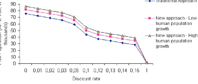
Using the Schaefer specification, we show graphically how the optimal fish population, x∞,
depends on the discount rate, δ, and the human population growth rate, n, (in formula (18)). We create graphs for fast growing (e.g., herrings) and slow growing (e.g., orange roughy) fish species, respectively, using the traditional and our new discounting approaches, more precise, we haved calculated the equilibrium population for a high growth fish specie with respect the discount rate for 3 cases: the traditional approach, our approach when the human population growths slowly, and our approach when it grows quickly.
We present in Figure 1 a graph showing how the optimal fish population changes for slow growing fish depending on the discounting approach used and the rate of growth of the human population. Figure 2 presents a similar graph for fast growing fish.
Some key observations from the figures are:
• Our new approach results in higher optimal fish populations for all discount rates; • The difference between the optimal fish population under traditional discounting and
hu-Figure 1: Optimal standing fish population for slow growing fish depending on the discounting approach used and the rate of growth of the human population.
Figure 2: Optimal standing fish population for fast growing fish depending on the discounting approach used and the rate of growth of the human population.
• Because human population growth hardly exceeded 5% (globally) recently, the effect of
our new approach declines as discount rates approach 5% in the case of slow growing fish and 15% in the case of fast growing fish.
4
Conclusion
We have shown that, in a very simple context where the human population grows at a constant rate n and all individuals have the same rate of time preference δ > 0, the main conclusion of the Schaefer model still holds, with δ, the individual rate of time preference, replaced by δ − n. This is a robust conclusion: indeed, it was reached by attaching a Pareto weight e−σt to the generation born at time t , and it turns out to be independent of σ. It
is also a reasonable one. When n = 0 for instance, so that the population is constant, each death being exactly balanced by one birth, so that whenever one individual disappears, an identical one arises in his/her place. It is then natural to consider this dynasty as a single individual living for ever, and having a rate of time preference equal to δ. Of course, one then forgets that transfers across time are really transfers across individuals. Our result shows that it is of no consequence for the equilibrium stock x∞.
Applying our new approach to slow and fast growing fish species under different assump-tions of human population growth rates, we demonstrate that our new approach means (i) higher optimal fish populations for all discount rates, for both slow and fast growing fish; and (ii) the difference between the optimal fish population under traditional discounting and our new discounting approach is largest for slow-growing fish, especially when the human population growth rate is high.
Our argument extends beyond the example of fisheries to the management of renewable resources in general. Take forestry for instance. The stock of trees is a public good, and if one considers the value of the harvest to be a proxy for the value of that public good, one is led to the same problem, where x now is the stock of trees instead of the stock of fish. More generally, when evaluating long-term projects, the consequences of which will be felt over several generations, we feel it is inappropriate to discount costs and benefits at the market rate ρ, which reflect the time preference of individuals. To take into account the impact of such projects on future generations, one should lower the interest rate, and the present paper suggests that it should be replaced by ρ − n, where n is the growth rate of the human
population.
Of course, this has been proved only in a special case, and there are other effects to take into account. Some of them also tend to lower the long-term interest rate; in that category, we find the various types of uncertainty (on the growth rate [20], on the model [21]) and the heterogeneity of the individual rates of time preference accross the population [11]. Others, such as the growth rate of consumption, go in the other direction: if we believe that our descendants will be wealthier than we are, then the discount rate we use for intertemporal welfare should be increased. In real-life situations, where there is likely to be an increase in consumption goods and a decrease in environmental goods, the balance will be hard to strike. The scope of this paper has been restricted to the impact of intergenerational equity, and there remains much work to be done.
References
[1] Barro, Robert and Sala-i-Martin, Xavier (1995) ”Economic growth”, Mc-Graw and Hill [2] Blanchard, Olivier and Fisher, Stanley (1994) ”Lectures on macroeconomics”, MIT Press [3] Clark, Colin (1973) ”Profit Maximisation and the Extinction of Animal Species”, Journal
of Political Economy 81, 950-61
[4] Clark, Colin and Lamberson, R. (1982) ”An Economic History and Analysis of Pelagic
Whaling. Marine Policy”, April 1982: 103-120.
[5] Clark, Colin (1990; second edition, 2005) ”Mathematical Bioeconomics”, Wiley
[6] Ekeland, Ivar and Lazrak, Ali (2006) ”Being serious about non-commitment: subgame
perfect equilibrium in continuous time” http://arxiv.org/abs/math/0604264
[7] Ekeland, Ivar and Lazrak, Ali (2008) ”Equilibrium policies when preferences are time
inconsistent”, http://arxiv.org/abs/0808.3790
[8] Harris, Christopher, and Laibson, David (2002) “Hyperbolic discounting and
consump-tion” eds. Mathias Dewatripont, Lars Peter Hansen, and Stephen Turnovsky, Advances in Economics and Econometrics: Theory and Applications, Eighth World Congress,
[9] Koopmans, Tjalling (1960) ”Stationary ordinal utility and impatience”. Econometrica 28, 287–309.
[10] Lind, Robert (1982) ”Discounting for time and risk in energy policy”, Resources for the Future, Washington, DC
[11] Nocetti, Diego, Jouini, Elyes and Napp, Clotilde (2008) ”Properties of the social discount rate in a Benthamite framework with heterogeneous degrees of impatience” Management Science 54 (10). 1822-1826
[12] Pauly, Daniel, Christensen, V., Guenette, S., Pitcher, T.J., Sumaila, U.R., Walters, C.J., Watson, R., Zeller, D. (2002) ”Towards sustainability in world fisheries”, Nature 418, 689–695.
[13] Portney, Paul and Weyant, John, editors (1999) ”Discounting and intergenerational
equity”, Resources for the Future, Washington D.C.
[14] Ramsey, Frank (1928) ”A mathematical theory of saving”, Economic Journal 38, p. 543-559
[15] Romer, David (1996), ”Advanced macroeconomics”, McGraw and Hill
[16] Schaefer, M.B. (1957) ”Some considerations of population dynamics and economics in
relation to the management of marine fisheries”, Journal of the Fisheries Research Board
of Canada 14, 669-681
[17] Stern, Nicholas (2007) ”The economics of climate change: the Stern review”. Cambridge University Press, 712p.
[18] Sumaila, U. Rashid (2004). ”Intergenerational cost benefit analysis and marine ecosystem
restoration”,. Fish and Fisheries, 5, 329-343.
[19] Sumaila, U. Rashid, and Walters, Carl (2005). ”Intergenerational discounting: a new
intuitive approach”, Ecological Economics 52, 135-142.
[20] Weitzman, Martin (2001) ”Gamma discounting”, American Economic Review 91 (1) p. 260-271
[21] Weitzman, Martin (2008) ”On modeling and interpreting the economics of catastrophic climate change”, American Economic Review 91 (1) p. 260-271
A
Appendix: Introduction
In the second part of this appendix, we prove Theorems 2 and 3. In the first part, we show how to associate with any threshold strategy h two functions v (x) and w (x), very similar to the value function in optimal control, and we study their differentiability properties. These functions will be helpful in characterizing equilibrium strategies and will be used to prove Theorems 2 and 3.
From now on, we will simplify the notations by writing the discount factor R (t) as follows:
R (t) = λe−δ0t+ (1 − λ) e−σ0t with: δ0:= (δ + ω) σ0:= (σ − n) λ := 1 − α α + δ − σ
B
Threshold strategies
Let h (t) be a threshold strategy (not necessarily an equilibrium strategy) converging to x∞.
Denoting, as above, by ξ(t, h, x) the stock at time t, when the fishing rate is h (t) and the initial stock is x, we introduce two functions which will play a crucial role:
v(x) := Z ∞ 0 λe−δ0t (p − c(ξ(t, h, x)))h(ξ(t, h, x))dt (21) w(x) := Z ∞ 0 (1 − λ)e−σ0t (p − c(ξ(t, h, x)))h(ξ(t, h, x))dt (22) so that the present value associated with a fishing rate h and the starting stock x, is V (h, x) =
v(x)+w(x). It is clear from the definition of a threshold strategy that v and w are continously
differentiable at every x 6= x∞. The case x = x∞ is important and will be handled directly.
B.1
The case x < x
∞We have h (x) = 0 and the fish stock is increasing. Let a small time τ > 0 elapse, so that the stock reaches the level x + ε < x∞, with ε = f (x)τ. We have, up to first order in ε:
v(x) = Z ∞ 0 λe−δ0t [p − c(ξ(t, h, x))]h(ξ(t, h, x))dt = Z τ 0 λe−δ0t [p − c(ξ(t))]h(ξ(t))dt + Z ∞ τ+ λe−δ0t [p − c(ξ(t))]h(ξ(t))dt = 0 + e−δ0τZ ∞ 0 λe−δ0t [p − c(ξ(t))]h(ξ(t))dt = e−δ0τv(x + ε) = µ 1 − δ0 ε f (x) ¶ (v (x) + εv0(x)) So v0(x) = δ 0 f (x)v (x) (23) and likewise: w0(x) = σ0 f (x)w (x) (24)
Adding up, we find that
(v0(x) + w0(x)) f (x) = δ0v(x) + σ0w(x) (25)
B.2
The case x > x
∞We have h (x) = hmaxand the fish stock is decreasing. Let a small time τ > 0 elapse, so that the stock reaches the level x − ε > x∞, with ε = (hmax− f (x)) τ. We have, up to first order in ε: v(x) = Z ∞ 0 λe−δ0t [p − c(ξ(t, h, x))]h(ξ(t, h, x))dt = Z τ 0 λe−δ0t [p − c(ξ(t))]hmaxdt + Z ∞ τ λe−δ0t [p − c(ξ(t))]h(ξ(t))dt = λ[p − c(x)]hmaxτ + e−δ0τv (x − ε) = λ[p − c(x)]hmaxτ + (1 − δ0τ ) (v (x) − εv0(x)) = v (x) + τ [λ (p − c(x)) hmax− δ0v (x) − (h max− f (x)) v0(x)] This leads to:
v0(x) = δ 0v(x) f (x) − hmax − λ p − c(x) f (x) − hmaxhmax (26) w0(x) = σ0w(x) f (x) − h − (1 − λ) p − c(x) f (x) − h hmax (27)
Adding up, we find that
(v0(x) + w0(x)) (f (x) − hmax) = δ0v(x) + σ0w(x) − hmax(p − c (x)) (28)
B.3
The case x = x
∞Start from a smaller stock x∞− ε, with ε > 0 small, and apply the strategy h. This means
that the fishing rate is h (t) = 0 until the level x∞ is reached again. This will happen after
a time τ = ε/f (x∞), and then the stock is stabilized at that level. This leads to:
v(x∞− ε) = Z ∞ 0 λe−δ0t (p − c(ξ(t, h, x∞− ε)))h(ξ(t, h, x∞− ε)))dt = Z ∞ τ λe−δ0t(p − c(x∞))f (x∞)dt = λ δ0e −δ0τ (p − c(x∞))f (x∞)
where we have taken into account that h(ξ(t, h, x∞− ε))) = 0 for 0 ≤ t ≤ τ . Hence the left
derivative:
v0−(x∞) = λ(p − c(x∞))
In the same way, we compute the right derivative. This time, we start with a larger stock
x∞+ ε, with ε > 0 small, and we apply the fishing level h (t) = hmax until the level x∞ is
reached again. This will happen after at time τ given by (hmax− f (x∞)) τ = ε. We have:
v(x∞+ ε) = Z τ 0 λe−δ0t (p − c(ξ(t, h, x∞+ ε)))hmaxdt + Z ∞ τ λe−δ0t (p − c(x∞))f (x∞)dt = λ(p − c(x∞))hmaxτ + e−δ 0τλ δ0(p − c(x∞))f (x∞) = v (x∞) + [λ(p − c(x∞))hmax− λ(p − c(x∞))f (x∞)] τ = v (x∞) + λ(p − c(x∞)) (hmax− f (x∞)) τ
and substituting the value for τ , we get v0
+(x∞) = λ(p − c(x∞)), which proves that the right
and left derivatives are equal, so that v is derivable at x∞, with v0(x∞) = λ(p − c(x∞)).
On the other hand, we also have:
v(x∞) =
Z ∞ 0
λe−δ0t(p − c(x∞))h(x∞))dt = λ
δ0h (x∞) (p − c (x∞))
(fishing rate maintains the stock at the level x∞), so that λ (p − c (x∞)) f (x∞) = δ0v (x∞).
equilibrium: v0(x∞) = λ(p − c(x∞)) (29) w0(x∞) = (1 − λ) (p − c(x∞)) (30) v (x∞) = λ δ0f (x∞) (p − c (x∞)) (31) w (x∞) = 1 − λ σ0 f (x∞) (p − c (x∞)) (32) Note that: v0(x∞) = δ 0 f (x∞)v (x∞) = δ0v(x ∞) f (x∞) − hmax − λ p − c(x∞) f (x∞) − hmaxhmax w0(x ∞) = σ 0 f (x∞)w (x∞) = σ0w(x ∞) f (x∞) − hmax − (1 − λ) p − c(x∞) f (x∞) − hmaxhmax
so that (23), (24), (26) and (27) all hold at x = x∞. As a consequence, so do (25) and (28)
C
Equilibrium strategies
C.1
Characterization
We now consider the (ε, t, a)-perturbation of h. Without loss of generality, we can assume that t = 0 (that is, we reset our watches if necessary), so that:
hε(s) = h(x(t)) ε < t a 0 ≤ t ≤ ε (33) Let us write vεand wεinstead of vhε and whε, so that v0= v and w0= w. Keeping only
first-order terms in ε, we have, at any point x 6= x∞:
vε(x) = Z ∞ 0 λe−δ0t [p − c(ξ(t, hε, x))]hε(ξ(t, hε, x))dt = Z ε 0 λe−δ0t [p − c(ξ)]hε(ξ)dt + Z ∞ ε λe−δ0t [p − c(ξ)]hε(ξ)dt = λ[p − c(x)]aε + Z ∞ 0 λe−δ0(t+ε)[p − c(ξ(t + ε))]h(ξ(t + ε))dt = λ[p − c(x)]aε + e−δ0ε Z ∞ 0 λe−δ0t[p − c(ξ(t + ε))]h(ξ(t + ε))dt = λ[p − c(x)]aε + (1 − δ0ε) v h(ξ (t + ε)) = vh(x) + ε [v0h(x) (f (x) − a) − δ0vh(c) + λ (p − c(x)) a]
The term (f (x) − a) comes from the fact that, if the fishing rate is a exerted during a period
ε when the stock is x, then the new stock at the end of the period will be x + (f (x) − a) ε,
up to first order. Similarly, we get:
wε(x) = w (x) + ε [w0(x) (f (x) − a) − σ0w (c) + (1 − λ) (p − c(x)) a]
We then introduce the Hamiltonian H (x, a):
H (x, a) := (v0(x) + w0(x)) (f (x) − a) − δ0v(x) − σ0w(x) + (p − c(x)) a (34)
= a [(p − c(x)) − (v0(x) + w0(x))] + (v0(x) + w0(x)) f (x) − δ0v(x) − σ0w(x) (35)
Condition (17) then reduces to the following:
max {H (x, a) | 0 ≤ a ≤ hmax} ≤ 0 (36)
By definition, h (x) is an equilibrium strategy if and only if it satisfies condition (36). It is reminescent of the classical Hamilton-Jacobi-Bellman equation in optimal control, so once again we emphasize that, in the present situation, with non-constant discounting, it will NOT give an optimal solution, but an equilibrium one.
In (36) we find ourselves maximizing a linear function of a, so the maximum must be attained at the boundary unless the slope is zero. There are two possible cases for x 6= x∞,
according to the value of the maximand h (x):
• if h (x) = 0, so that x < x∞, the slope must be negative or zero:
0 ≥ (p − c(x)) − (v0(x) + w0(x)) (37)
• if h (x) = hmax, so that x > x∞, the slope must be positive or zero:
0 ≤ (p − c(x)) − (v0(x) + w0(x)) (38)
C.2
Necessary condition: Theorem 2 .
We have proved that the function v and w are continuously differentiable everywhere. Con-ditions (37) and (38) mean that function ϕ (x) := v0(x) + w0(x) − p + c (x) goes from ≥ 0
to ≤ 0 when x increases through x∞. It is continous, and hence much vanish at x∞:
v0(x
We know that ϕ is differentiable all x 6= x∞, but we cannot assume that it is differentiable
at x∞. So we cannot claim that ϕ0(x∞) ≤ 0. However, there is a sequence xn −→ x∞from
the left (xn< x∞) and a sequence yn−→ x∞from the right (yn> x∞) such that ϕ0(xn) ≤ 0
and ϕ0(y n) ≤ 0:
v00(x
n) + w00(xn) ≤ −c0(xn) and v00(yn) + w00(yn) ≤ −c0(yn)
Let us work on the first equation. Differentiating (25) we have:
(v00(xn) + w00(xn))f (xn) + (v0(xn) + w0(xn))f0(xn) = δ0v0(xn) + σ0w0(xn)
Combining with the preceding inequation, we get: 1
f (xn)[δ 0v0(x
n) + σ0w0(xn) − (v0(xn) + w0(xn))f0(xn)] ≤ −c0(xn)
and taking the limit as n −→ ∞, we get: 1
f (x∞)
[δ0v0(x
∞) + σ0w0(x∞) − (v0(x∞) + w0(x∞))f0(x∞)] ≤ −c0(x∞) (39)
Now let us work on the yn. Differentiating (28) we have:
(v00(yn) + w00(yn)) (f (x) − hmax) + (v0(yn) + w0(yn))f0(yn) = δ0v0(yn) + σ0w0(yn) + hmaxc0(yn)
Combining with the inequality ϕ0(y
n) ≤ 0, and taking the limit as n −→ ∞, we get:
1 f (x) − hmax[δ 0v0(x ∞) + σ0w0(x∞) + hmaxc0(x∞) − (v0(x∞) + w0(x∞))f0(x∞)] ≤ −c0(x∞) (40) δ0v0(x∞) + σ0w0(x∞) − (v0(x∞) + w0(x∞))f0(x∞) ≥ −f (x∞) c0(x∞)
Combining (39) and (40), we find:
δ0v0(x
∞) + σ0w0(x∞) − (v0(x∞) + w0(x∞))f0(x∞) = −f (x∞) c0(x∞)
Plugging in the values for v0(x
∞) and w0(x∞) from (29) and (30), we find:
C.3
General growth and cost: Theorem 3
As in section 3.3, we define v and w by (21) and (22). Differentiate equations (23) and (24) from the left at x∞:
v00 −(x∞) = v0(x∞)δ 0− f0(x ∞) f (x∞) = λ(p − c(x∞))(δ0− f0(x∞)) f (x∞) w00 −(x∞) = w0(x∞)σ 0− f0(x ∞) f (x∞) = (1 − λ)(p − c(x∞))(σ0− f0(x∞)) f (x∞)
Set I(x) = f (x)(p − c(x)) and ψ(x) = v(x)δ0+ w(x)σ0− I(x). Note that, by (29), (30),
(31) and (32), we have:
ψ(x∞) = 0 = ψ0(x∞)
Now consider the (left) second derivative ψ00
−(x∞).After some computations, we find:
ψ−00(x∞) = µ δ0λ(p − c(x∞))(δ 0− f0(x ∞)) f (x∞) + σ 0(1 − λ)(p − c(x∞))(σ0− f0(x∞)) f (x∞) − I 00(x ∞) ¶ = (δ0A + σ0B − I00(x ∞))
with obvious notations. Note that A + B = −c0(c
∞) by (41). Since σ0 > 0 and f0(x∞) < 0
by hypothesis, follows that AB ≥ 0; moreover A + B ≥ 0 because c (x) has been assumed to be decreasing. It follows that A and B are positive, and hence:
ψ−00(x∞) ≥ − min(δ0, σ0)c0(x∞) − I00(x∞) > 0
So there exist some a < x∞ such that ψ(x) > 0 for all x in the open interval ]a, x∞[.
We redo the preceeding analysis but for x > x∞. We find:
v00 +(x∞) = λc 0(x ∞)hmax+ λ(p − c(x∞))(δ0− f0(x∞)) f (x∞) − hmax w+00(x∞) = (1 − λ)c0(x ∞)hmax+ (1 − λ)(p − c(x∞))(σ0− f0(x∞)) f (x∞) − hmax and hence: ψ00+(x∞) = −(p − c(x∞))λδ 0(δ0− f0(x ∞)) + (1 − λ)σ0(σ0− f0(x∞) ¯h − f(x∞) − µ (λδ0+ (1 − λ)σ0)c0(x ∞)¯h ¯h − f(x∞) + I 00(x) ¶ ≥ − (min(σ0, δ0)c0(x ∞) + I00(x∞)) > 0
As above, there exists b > x∞ such that ψ(x) > 0 for all x such that b > x > x∞. So,
this yields:
v0(x) + w0(x) =v(x)δ
0+ w(x)σ0
f (x) ≥ p − c(x) for a < x < x∞
while using (26) and (27), we get:
v0(x) + w0(x) = −[p − c(x)]hmax+ δ0v(x) + σ0w(x)
f (x) − hmax ≤ p − c(x) for x∞< x < b But these two inequalities are precisely (37) and (38). So the threshold strategy converging to x∞ is an equilibrium strategy, as announced.