Originate-to-Distribute and Screening Incentives

Originate-to-Distribute and Screening Incentives

Gilles Chemla

Imperial College Business School, DRM/CNRS, and CEPR.

Christopher A. Hennessy

London Business School, CEPR, and ECGI.

March 2011

Abstract

Conventional wisdom holds that lax screening during the subprime boom was the inevitable result of the originate-to-distribute (OTD) business model under which originators retain zero interest in complex tranched securities (CDOs). This has led to calls for originators to main-tain more skin-in-the-game (SITG) and curbs on CDOs. We examine these claims in a fully rational model where originators first choose screening effort and then use private information regarding value in deciding between signaling via retentions versus pooling at OTD cum opti-mally structured CDOs. Contrary to conventional wisdom, we show screening incentives can actually be stronger under OTD, but only if two conditions are met: orginators attach high value to immediate funding and informed trading drives prices sufficiently close to fundamentals. We argue that lax lending standards during the subprime boom can be understood as arising endogenously from insufficient informed trading in CDO markets. Limits on tranched CDOs are shown to be misguided. Tranching creates Arrow securities demanded by hedgers who serve as trading partners for informed speculators who drive prices closer to fundamentals. We also show that screening and no screening by originators can be self-fulfilling prophecies as changes in the probability distribution of CDO quality shift incentives for information acquisition. Finally, we show that bans on shorting alter speculator trading capital needs, decreasing (increasing) the informational efficiency of prices if the unconditional expected quality is high (low).

“We must look at the price system as such a mechanism for communicating informa-tion. . . ” F.A. Hayek, 1945.

“Sometimes markets err big time... Selectively shorting the most problematic mortgage-backed securities in history today amounts to just such an opportunity.” Michael Burry, letter to his investors, October 2005.

It is commonly argued that the decline in lending standards prior to the subprime crisis of 2007/8 was inevitable given the preceding shift from relationship banking to the originate-to-distribute (OTD) business model under which lenders packaged pools of RMBS into complex tranched securi-ties (CDOs). This narrative has gained traction with policymakers, leading to calls for mandating more skin-in-the-game (SITG) and/or bans on CDOs.

Existing theoretical models are consistent with the notion that lender laxity is a necessary consequence of OTD. For example, see Gorton and Pennacchi (1995), Parlour and Plantin (2008), Plantin (2010), and Rajan, Seru and Vig (2010). After all, so the argument goes, an originator has no incentive to screen if he is going to sell all claims on cash flow at a price reflecting unconditional expected quality—the so-called pooling price. And indeed, in these models prices are equal to the pooling price precisely because traders are assumed to be incapable of generating information about loan quality.

In reality, traders can generate useful information and securities prices can be informative. After all, some hedge fund managers did generate information—simply by reading CDO prospectuses. In so doing, they eventually moved prices and the subprime engine froze. This suggests lender laxity was not an inevitable by-product of OTD cum CDOs. Rather, it suggests lender laxity arose from the failure of securities markets to price claims in a way that rewarded diligent originators for screening. To borrow Hayek’s terminology, the core cause of lender laxity was the failure of the price system.

The above argument illustrates that understanding screening incentives requires understanding the determinants of the informational efficiency of CDO prices. To that end, we develop a fully rational model in which an originator can screen at a cost in order to increase the probability of

a high cash flow. In the next period, the originator privately observes the true asset value (type below),  or , and chooses between separating via retention of risk (SITG), or pooling at full securitization (OTD). Under either choice, optimal tranching is employed. The main difference between our model and those discussed above is that we allow for the possibility of informed trading in optimally tranched claims driving prices closer to fundamentals.

In the event of separation using SITG, all claims are priced at fundamentals and the originator underinvests. In the event of pooling at OTD, investors trade claims in competitive markets popu-lated by rational uninformed investors (UI below) and a speculator. UI buy claims in order to hedge endowment risks, scaling back their trades in light of exposure to adverse selection. The speculator exerts costly effort in order to increase the precision of her signal regarding asset type. She then hides her trades behind the UI in order to confound market-makers.

A number of novel findings emerge from the model. First, we show that the OTD business model actually generates stronger screening incentives than SITG iff: originators attach sufficiently high value to immediate liquidity and informed trading drives prices sufficiently close to fundamentals. This is consistent with the preceding informal argument that the fundamental cause of lender laxity during the subprime boom was uninformative pricing.

Our second important result is to show that tranching increases the informational efficiency of prices, implying that bans on tranched CDOs could actually weaken screening incentives. Third, we show the optimal tranching structure features a riskless senior tranche and a risky junior tranche paying zero if the realized asset value is low. Intuitively, the objective of tranching is to carve out the type of Arrow claims most preferred by the uninformed hedgers. This stimulates UI demand, allowing the speculator to trade more aggressively and make larger gains. Anticipating this, the speculator exerts more effort and price informativeness increases.

Fourth, we show that both good and bad equilibria can be self-fulfilling for specified parameter values. In the former, the speculator exerts high effort anticipating a high probability of high asset value. In turn, the originator screens given informative pricing. In the bad equilibrium,

the speculator exerts low effort anticipating mostly lemons. In turn, this justifies the originator’s decision to forego screening given noisy pricing. Arguably, the loan market was trapped in this bad equilibrium during the subprime boom.

Finally, we use the model to evaluate the effect of short-sales restrictions on informational efficiency. Interestingly, a short-selling ban has no effect on informational efficiency if the speculator has no binding constraint on her trading capital. However, if she faces a binding constraint, a short-selling ban can decrease or increase informational efficiency depending on the relative trading capital required for long and short positions. A short-selling ban decreases (increases) informational efficiency if the probability of high quality is high (low). Intuitively, shorting (buying) is the cheapest way to express a view when other investors have a high (low) prior.

We turn now to a discussion of closely related papers. Gorton and Pennacchi (1995) show fractional retentions and implicit guarantees can increase screening incentives. Plantin (2010) argues that increased loan sales, and lax screening, can be understood as a constrained-efficient response to banks having better investment opportunities. Rajan, Seru and Vig (2010) develop and test a model in which lenders exert less effort acquiring soft information if the exogenous probability of full securitization is higher. As mentioned above, our model differs from each of these models in that we allow informed speculation to drive prices away from the uninformed pooling price and analyze optimal tranching designed to increase speculator incentives.

Our model is perhaps closest to that of Parlour and Plantin (2008). However, we follow Plantin (2010) in assuming the bank has a known positive NPV project with probability one. In contrast, in the model of Parlour and Plantin the bank has a stochastic investment opportunity set. If no project emerges, the bank will hold the loan until maturity, providing some screening incentive. If a project does emerge, the bank sells only if the uninformed pooling price is sufficiently high. But in such cases, screening incentives are undermined by the loan sale since the price is uncorrelated with fundamentals. The key difference is that in our model informed speculation creates a correlation between price and fundamentals, with optimal tranching increasing that correlation. Thus, screening

incentives can be provided even with full securitization.

Boot and Thakor (1993) analyze security design in a pure hidden information setting with no screening. They show tranching can stimulate speculator effort, but focus on a different lever. In their model, tranching relaxes speculator wealth constraints as they trade against pure noise traders. Fulghieri and Lukin (2001) also analyze the role of security design in a similar setting.

In the model of Gorton and Pennacchi (1990), uninformed investors carve out safe tranches in order to furnish themselves with a safe storage technology. Hennessy and Chemla (2011) show that a privately informed bank would not issue a safe claim in such a setting, relying on uninformed trade in risky debt to promote informed trading. Both papers abstract from screening incentives. Further, the theory of security design derived in the present paper differs fundamentally in that here uninformed investors trade in the risky junior tranche in order to hedge endowments negatively correlated with asset value.

Dang, Gorton and Holmström (2010) and Hanson and Sunderam (2010) also analyze the link be-tween security design and information acquisition. In these models, debt claims have low informational-sensitivity during good times and speculators do not acquire information. In the former model, speculators acquire information in bad times, with adverse selection causing no-trade. In the latter model, the securitization market freezes in bad times since investors did not invest in slow-moving information systems during the boom. Both models abstract from screening incentives, the primary focus of our paper.

Shleifer and Vishny (2010) present a behavioral model in which securitization volume increases in response to an exogenous price exceeding fundamental value. Although their model is silent on screening incentives, it is worth pointing out that overoptimism in securities markets need not destroy screening incentives. For example, proportional overvaluation of all securities actually increases screening incentives by increasing the absolute wedge between high and low type payoffs.

The role of price informativeness in alleviating moral hazard has been analyzed in other con-texts. Holmström and Tirole (1993) present a model in which the equity float affects information

acquisition, price informativeness, and managerial risk premia. Maug (1998), Aghion, Bolton and Tirole (2004) and Faure-Grimaud and Gromb (2004) show that price informativeness stemming from speculator monitoring promotes insider effort. These papers are necessarily silent on the trade-offs of OTD versus SITG. Further, only Aghion, Bolton and Tirole analyze security design. And most fundamentally, each of these papers assumes pure noise trading, precluding the use of tranching to increase uninformed demand and the gains to informed speculation.

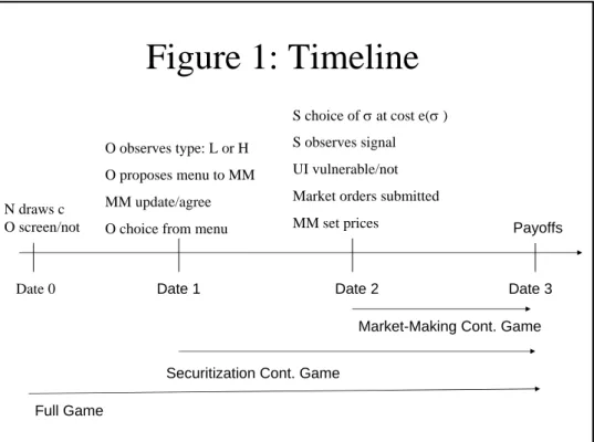
The remainder of the paper is as follows. Section I describes the full game and timing. Section II analyzes the final continuation game in which market-makers set prices. Section III analyzes the penultimate continuation game in which the privately informed originator chooses between signaling via retentions versus pooling at full securitization. Section IV compares screening incentives under SITG and OTD. Section V pins down the optimal tranching structure. Section VI describes the effect of short-selling on speculator incentives.

I. The Game

This section describes the structure of the Full Game, which itself features two proper continu-ation games. The equilibrium concept is perfect Bayesian equilibrium (PBE). A PBE demands: all agents have a belief at each information set; strategies must be sequentially rational given beliefs; and beliefs are determined using Bayes’ rule and the equilibrium strategies for all information sets on the equilibrium path.

A. Screening Technology and Agent Preferences

There are four periods, 0 1 2 and 3 with the Full Game starting at  = 0 In the last two periods, there is a single storable consumption good. Originator is time and risk-neutral, deriving utility from consumption equal to 2+ 3

At the start of period 0, Nature publicly draws a screening cost  from an atomless cumulative distribution  having strictly positive density  on the support [0 ∞) Originator then decides whether to pay the non-pecuniary effort cost  in order to screen prospective borrowers. Effort is

not publicly observable but is correctly inferred in equilibrium. Screening increases the quality of the underlying asset, e.g. a loan or pool of loans. If Originator screens, the underlying asset delivers  with probability  and  with probability 1_{− If he does not screen, the asset instead delivers } with probability  and  with probability 1_{−  The equilibrium value of  is denoted }_{ The cash}

flow generated by the underlying asset accrues at time 3 Throughout it is assumed that 0   1 and  ∈ (0 )

At the beginning of period 1, Nature draws the true payoff (type)  ∈ { } of the underlying asset from the appropriate -contingent distribution given the screening decision at date 0. Origi-nator privately observes  and is the only agent endowed with perfect knowledge of the asset type. The originator attaches a value   1 to each unit of funding he raises in securities markets at time 2. To fix ideas, throughout we treat the originator as having access to a new scalable investment with an expected payoff of  units at time 3 per unit invested at time 2. Alternatively, one can think of  as measuring the shadow value of liquidity for a bank facing capital adequacy tests. As in Parlour and Plantin (2008) and Plantin (2010),   1 encourages securitization.

Agents receive endowments and consume at dates 2 and 3 They can store their date 2 endowment in order to carry resources to date 3, or they can buy securities sold by the originator. In the baseline model, we follow Allen and Gale (1988) in assuming limitations on the verifiability of endowments leads to endogenously incomplete markets. In particular, the endowments of the various agents are not verifiable by courts. Consequently, other agents cannot issue securities, borrow or short-sell. Section VI analyzes the effect of short-selling.

In the baseline model, the only verifiable quantity is the cash flow generated by the underly-ing asset originally owned by Originator. In contrast, courts cannot verify the payoff on the new investment opportunity. This distinguishes our securitization model from a model of optimal fi-nancial structure for a corporation, since the latter features claims written on both assets in place and growth options. In our setting, the originator sells claims on the underlying asset in order to increase the scale of the new investment.

There is a continuum of uninformed investors (UI) having measure one. UI may have an insurance motive for purchasing securities delivering consumption at date 3. The UI are sufficiently wealthy in aggregate to buy the entire asset at date 2 since each has a date 2 endowment ₂ _{≥ }

UI face a common endowment shock, with their date 3 endowment 

3 being either  or −  0

Just prior to securities market trading in period 2 UI privately observe a signal regarding their date 3 endowment. In particular, with probability one-half they find that they are “invulnerable” to a negative shock and will have endowment ₃=  with probability one. With probability one-half they are “vulnerable” to a negative shock. The endowment shock is negatively correlated with the value of the underlying asset, creating a natural hedging demand. Conditional upon being vulnerable, if the underlying asset delivers  the date 3 endowment will be  −  and if the underlying delivers  the date 3 endowment will be 

In fact, this setup is a reduced-form representation of hedging clienteles in housing markets. To see this, consider agents who invest in assets at date 2 in order to buy a (necessity) house and a consumption good at date 3. For such agents, mass defaults in the final period are good news since such an outcome would allow them to buy houses cheaply. Conversely, low defaults are associated with higher house prices. One can then think of  as capturing the negative shock to non-housing consumption that hits prospective home buyers if defaults are low. Long positions in CDOs help such agents hedge.

UI are risk-neutral over date 2 consumption and risk-averse over date 3 consumption, with  being a critical threshold for final period consumption. They are indexed by the intensity of their risk-aversion as captured by a preference parameter . The utility of uninformed investor- takes the form:

 (2 3; ) ≡ 2+  min{3−  0} (1)

The preference parameters have compact support Θ ≡ [1 max] Throughout, max is assumed to be sufficiently high such that there is always strictly positive uninformed demand for at least one

security.1 The  parameters have density  with cumulative density  This distribution has no atoms, with  being strictly positive and continuously differentiable. This tractable specification of risk-aversion is also used by Dow (1998). Other smooth utility functions could be assumed at the cost of more complex aggregate demand functions. The essential assumption is that UI are risk averse over final period consumption, so they are potentially willing to buy claims issued by Originator despite facing adverse selection in securities markets.

There is a risk-neutral speculator  with utility 2+ 3. At date 2 she is endowed 2 ≥ 

units of the numeraire, so she can afford to buy the entire asset. Her final period endowment is normalized at zero in the baseline model. The speculator is unique in that she receives a noisy signal of asset type and can exert costly effort to increase signal precision. Letting  ∈ { }

denote the signal and  the true asset type,  chooses  ≡ Pr( = ) from the feasible set [12 1]

Her non-pecuniary effort cost function  is strictly positive, strictly increasing, strictly convex, twice continuously differentiable, and satisfies

lim ↓12 () = 0 lim ↓12 0() = 0 lim ↑1  0_{() = ∞}

If  exerts effort, the signal becomes informative since

  1 2 ⇒ Pr[ = | = ] = Pr[ =  ∩  = ] Pr[ = ] =   + (1 − )(1 − )   (2) The final set of agents in the economy is a continuum of deep-pocketed market-makers having measure one. They are risk-neutral and have utility equal to 2+ 2.

B. The Securitization Game

Since Originator is privately informed regarding the true value of the underlying asset at the start of period 1, his choice of retention and security design is a signaling game. Maskin and Tirole

1

(1992) and Tirole (2005) show the equilibrium set of such games can be narrowed and Pareto-improved (from the perspective of the privately informed party) by expanding the set of feasible initial actions. We adapt the game of Tirole (2005) to our setting.

The sequencing of events is as follows. The continuation game starting at date 1 is called the Securitization Game. It is a signaling game played between Originator and outside investors. This game begins with the privately informed Originator approaching market-makers (e.g. investment banks) and publicly proposing a menu of two securitization structures, say Σ ∈ {Σ Σ}, that he

would like the option to choose from subsequently, e.g. a shelf-registration. Each structure stipulates payoffs for claimants as a function of the verifiable asset payoff at date 3. The market-makers then agree to clear markets competitively for whatever structure the originator subsequently chooses from the menu. All agents must have a belief regarding the asset type in response to any menu offer, including those off the equilibrium path. Thus, the menu offered is itself a potentially informative signal.

Next, the originator selects a securitization structure Σ from the menu he just proposed, with the choice being incentive compatible. After observing Originator’s choice, all agents revise beliefs using Bayes’ rule where possible. It is worth stressing that both types can offer the same menu, but they do not necessarily select the same securitization structure. In a separating equilibrium, the initial menu is such that the securitization structure chosen by the originator reveals the true asset type. In a pooling equilibrium, both originator types propose the same trivial menu with Σ = Σ

In pooling equilibria, no information about the type can be inferred based upon the securitization structure chosen by the originator.

C. The Market-Making Game

At date 2, play passes to a second continuation game, labeled the Market-Making Game.2 In this game, prices of claims are set competitively by the market-makers facing the potentially-informed speculator. In a separating equilibrium, the true type has been revealed, so prices are set equal to

2

fundamental value, and the speculator does not exert effort.

Consider next a pooling equilibrium. In this case, the Market-Making Game is a signaling game played between the informed speculator and market-makers. Here, the market-makers and unin-formed investors enter the market-making game holding their prior belief that the asset has high payoff with probability  ∈ { } with  (and screening effort) being correctly inferred in equilib-rium. The market-making game starts with  choosing  at personal cost (). Her equilibrium choice  is not publicly observable, but is correctly inferred by other agents in equilibrium. Then  privately observes her signal  ∈ { } regarding the asset type.

Next, UI privately observe whether or not they are vulnerable to a negative endowment shock at date 3. Market orders are then submitted, with market-makers setting prices competitively. The market-making process is in the spirit of Kyle (1985) and Glosten and Milgrom (1985). The speculator and uninformed investors simultaneously submit non-negative market orders. Market-makers then set prices based upon observed aggregate demands in all markets, with no market segmentation. Market-makers clear all markets, buying all securities not purchased by UI or S.

Since Originator is the only agent capable of issuing claims delivering goods in period 3, market-makers cannot be called upon to take short positions. To this end, we impose the following technical assumption.

1 :  ≤  − ₂ 

The role of Assumption 1 is as follows. The aggregate demand of UI is weakly increasing in . To avoid the possibility of aggregate demand exceeding supply for any security, the endowment shock must be sufficiently small.

Figure 1 provides a time-line.

II. Equilibrium of Market-Making Game

We solve for the set of PBE of the Full Game via backward induction. Consider first the Market-Making Game. This game is trivial in a separating equilibrium since in that case all securities will

be priced at fundamental value given the revealed type. Therefore, we confine attention below to analyzing pricing in pooling equilibria—where both issuer types pool at the same trivial menu and structure. We initially abstract from optimal security design, considering first the case in which the originator packages and sells the entire asset in the form of a pass-through security. This allows us to isolate the role of tranching in Section V.

Since she cannot short-sell, the optimal strategy for Speculator is to place a buy order if and only if she receives a positive signal. She attempts hiding her buy orders behind those of the UI. The optimal size of her buy order is equal to the size of the aggregate buy order placed by UI when they are vulnerable to negative endowment shocks. This latter quantity is denoted  and is determined endogenously.

UI do not place any orders if invulnerable to negative shocks since the marginal utility of any increase in 3 is then zero. An individual UI may place a buy order if vulnerable since there is a

hedging motive. However, UI are rational, weighing adverse selection costs against hedging motives in determining optimal demand. Each UI conditions demand on his preference parameter .

Table 1 lists the possible aggregate demand () configurations confronting market-makers. Using Bayes’ rule, market-makers form the following beliefs

Pr[ _{= | = 2] =} 

1 −  −  + 2 (3)

Pr[ _{= | = ] = }

Pr[ _{= | = 0] =} (1 − )  +  − 2

Market-maker beliefs and equilibrium prices ( ) increase monotonically in aggregate demand with:

 () = _{ + ( − ) Pr[ = |] ∀ ∈ {0  2}} (4)

⇒  (2)   ()   (0)

To support the PBE conjectured in Table 1 it is sufficient to verify the speculator has no incentive to deviate regardless of the signal she receives. To that end, off the equilibrium path market-makers

form adverse beliefs from the perspective of the speculator, setting prices based upon: Pr[ = |] = 1 ∀  ∈ {0  2}

It is readily verified that the speculator has no incentive to change her signal-contingent trading strategy when confronted with such beliefs. While such beliefs off the equilibrium path are sufficient to support the conjectured PBE of the market-making game, it is worthwhile to briefly discuss their plausibility. Note that any  _{∈ {0  2} must be due to the speculator placing a strictly positive} order. The chosen specification of beliefs off the equilibrium path is predicated on the intuitive notion that market-makers should view any such (positive) order as being placed by  after having observed . After all, if a negative signal is received, the speculator stands to incur a loss from

buying securities unless the market-makers form the most favorable beliefs from her perspective, which would entail Pr[ = |] = 0. Conversely, if a positive signal is received, the speculator

stands to make a strictly positive trading gain provided Pr[ = |]  1

A. Expected Revenue of Originator

Using Table 1 we compute the expected revenue of the high type originator as:

[] =  + ( − ) ∙  Pr[ = | = 2] 2 + (1 − ) Pr[ = | = 0] 2 + Pr[ = | = ] 2 ¸  (5) Equation (5) can be rewritten as:

[] = ( ) + [1 − ( )] (6) ( ) ≡ 1₂ ∙ 2 1 −  −  + 2 + (1 − )2  +  − 2 +  ¸ 

The variable  plays a critical role, measuring the high type’s expectation of the market-makers’ updated belief. For example, if it were possible to achieve  = 1 then there would be no mispricing. From Bayes’ rule one can relate the expected revenue of the low type to that of the high type as follows

which implies [] = ( ) + [1 − ( )] (8) ( ) ≡ µ  1 −  ¶ [1 − ( )]

Lemma 1, proved in the appendix, shows the high type benefits from higher speculator signal precision, since higher precision drives prices closer to fundamental value.

Lemma 1 The expected revenue of the originator of a high value asset is increasing in the precision of the signal received by the speculator.

From Lemma 1 it follows that  is increasing in , with  µ 1 2 ¶ =  (9) (1) = 1 +  2 

It is worth noting that if Speculator fails to exert effort ( = 12), then  =  and the expected revenue of each type reverts to the unconditional expected payoff as in standard existing models. B. Incentive Compatible Information Acquisition

Consider next the incentives of Speculator. From Table 1 it follows that her expected gross trading gain is (  ) =  · ⎡ ⎢ ⎣ ¡ 2 ¢ [ −  (2)] +¡2 ¢ [ −  ()] + ³ (1−)(1−) 2 ´ [ −  (2)] + ³ (1−)(1−) 2 ´ [ −  ()] ⎤ ⎥ ⎦ (10) = (1 − )(2 − 1)( − ) 2

The incentive compatible signal precision, denoted , satisfies the first-order condition:

0() = (1 − )( − ) (11)

Since the incentive compatible signal precision plays a critical role, we summarize its properties, which follow directly from applying the implicit function theorem to the speculator’s first-order condition:

Lemma 2 The incentive compatible signal precision of the speculator is increasing in the aggregate demand of the uninformed investors when vulnerable (); increasing in the wedge between the value of the claim under high and low types; increasing in  for   12; and decreasing in  for   12

C. Uninformed Demand for the Pass-Through Security

The next step is to determine aggregate UI demand () for the pass-through security in response to their being vulnerable to a negative endowment shock, recalling that the UI have zero demand if invulnerable. Letting ∗_{() denote the optimal -contingent demand, aggregate uninformed demand}

is

 ≡ Z max

1

∗() () (12)

Each UI has measure zero and acts as a price-taker. Each vulnerable UI expects the security to be overpriced since he knows a subset of fellow vulnerable UI will be submitting positive demands, pushing prices higher as market-makers revise upward their assessment of the probability of the asset being of high value. Despite facing adverse selection, an individual UI is willing to submit a buy order if  is sufficiently high.

In order to characterize UI demand, it is useful to compute the expected price of the secu-rity conditional upon the UI being vulnerable to a negative endowment shock. This conditional expectation, computed by each UI, is:

 _{= [ + (1 − )(1 − )] (2) + [(1 − ) + (1 − )] ()} (13) =  + (1 − ) + (1 − )(2 − 1)( − )

Equation (13) is consistent with the intuition that UI face adverse selection when submitting buy orders, since the asset is overpriced relative to its unconditional expected value. Additionally, the equation reveals there is no adverse selection if the speculator does not exert effort ( = 12), with adverse selection increasing in her signal precision.

Consider now the optimal portfolio for an individual vulnerable UI. He will not invest his endow-ment in the safe storage technology since this is an inefficient means of insuring himself given that he

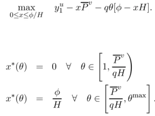
actually prefers an Arrow security paying off in the event that the realized payoff on the underlying asset is  We now let  denote the number of units of the pass-through security purchased, and confine attention to  ≤  since  in excess of that cutoff has zero marginal utility in the final period. The objective of each vulnerable UI is to solve:

max 0≤≤   1 −   − [ − ] (14) It follows that: ∗() = 0 _{∀  ∈} " 1   ! ∗() =   ∀  ∈ "    max # 

Lemma 3 summarizes the properties of aggregate uninformed demand.

Lemma 3 If types pool by selling the underlying asset in the form of a pass-through security, ag-gregate uninformed demand when vulnerable to a negative endowment shock is

() =   · ∙ 1 −  µ 1 + (1 − )(2 − 1) + µ 1 −   ¶ µ   ¶ (1 − (2 − 1)) ¶¸ 

Figure 2 sketches the proof for existence of a unique equilibrium in the Market-Making Game (although the Full Game starting a date 0 does not necessarily have a unique equilibrium). To under-stand the figure, recall the incentive compatible signal precision from Lemma 2 and the uninformed demand from Lemma 3. Aggregate uninformed demand is a downward sloping function of  since more precise speculator signals worsen the adverse selection problem as perceived by UI. Plotting aggregate demand, we know (12)  0 and that  is strictly decreasing in  on [12 1] Plotting the incentive compatible signal precision, we know is strictly increasing in  with −1 (12) = 0,

with the limit as_{b converges to one of }−1_ (_{b) = ∞ Thus, the two curves intersect once, and only} once, implying a unique equilibrium.

Proposition 1 In the Market-Making Game following pooling of originators, there exists a unique equilibrium pair ( ) satisfying

() = ∈ µ 1 2 1 ¶ () = _∈ µ 0   ¶ 

III. Equilibrium of the Securitization Game

Continuing with the backward induction, suppose play has reached the Securitization Game. At the start of this game, all players have correctly inferred _{ However, Originator is privately}

informed about the true asset payoff. This sets up a signaling game in which Originator can either separate (by keeping sufficient skin-in-the-game) or pool by selling all of the underlying asset (originate-to-distribute) in the form of a pass-through security.

Originator credibly signals positive private information by retaining sufficient rights. To this end, assume Originator designs a security  with value-contingent payoffs ( ) Originator

retains security  and sells the remaining cash flows to the market. Since all that matters in the case of separation is Originator’s risk exposure, we may assume without loss of generality that all such remaining cash flows are bundled into a single security, say security 

We begin by evaluating the least-cost separating equilibrium (LCSE). The LCSE minimizes the low type’s incentive to mimic by giving him his first-best allocation in which he sells the entire asset in the form of a pass-through security. The LCSE makes the high type as well off as possible subject

to the constraint that the low type does not want to mimic. The LCSE solves: max () +       :  ≥ +     

To determine the LCSE, we first ignore the monotonicity constraint and then verify it is slack. Clearly, in this relaxed program the optimal policy is to loosen the no-mimic constraint to the maximum extent by setting ∗_= 0 implying _∗ =  Further, the no-mimic constraint must bind at the optimum, implying _∗ =  and ∗_{ =  −  Since the neglected monotonicity constraint} is satisfied we have established the following proposition.

Proposition 2 In the least-cost separating equilibrium of the Securitization Game, a low type asset is sold in its entirety in the form of a pass-through security. The originator of a high type asset sells only a riskless senior (debt) claim with face value  retaining the residual (levered equity) claim.

The intuition behind Proposition 2 is simple. In the LCSE, the low type would always mimic if the high type were to sell any risky claim since he would then benefit from security overvaluation. Therefore, the best the high type can do is to get the maximum liquidity possible subject to zero informational-sensitivity. Debt with face value  achieves this objective.

In the LCSE, the high type experiences a loss relative to symmetric information equal to ( − 1)( − ) As in the model of Myers and Majluf (1984), in the LCSE asymmetric information results in the high type cutting back the scale of his investment and foregoing some positive NPV investments.

Lemma 4 The equilibrium set of the Securitization Game always includes the least-cost separating equilibrium. It also includes pooling equilibria with a single contract on the offered menu provided that contract weakly Pareto dominates the least-cost separating equilibrium (from the perspective of both owner types).

Proof. Consider first supporting the LCSE. If beliefs were set to Pr[ = ] = 0 in response to any deviating menu, then no such deviation is profitable. Suppose next there is a pooling contract weakly Pareto dominating the LCSE. If beliefs were set to Pr[ = ] = 0 in response to any deviating menu, the deviator would get weakly less than his LCSE payoff and the deviation is not profitable.

IV. Originate-to-Distribute versus Skin-in-the-Game

This section compares screening incentives under the separating equilibrium with a candidate pooling equilibrium in which the entire asset is packaged and sold off in the form of a pass-through security. The former represents skin-in-the-game and the latter represents originate-to-distribute. A. Is Originate-to-Distribute an Equilibrium Security Design?

We first determine conditions under which pooling at OTD can be supported as an equilibrium in the Securitization Game. Recall that Lemma (4) established that a pooling equilibrium can be supported provided that both types are weakly better off than under the LCSE. Clearly, the low type is better off under the posited pooling equilibrium since overpricing of his security ensures he will get strictly more than his LCSE payoff of  The high type is weakly better off in the pooling equilibrium than in the LCSE iff:

[] ≥  −  +  ⇔ [∗() ] ≥ −1 (15)

beliefs with the probability of the asset being of high value.

 _{≡ [}∗() ]  _{≡ [}∗() ]  _{≡ [}∗() ]

 _{≡ [}∗() ]

Using the above shorthand we have established the following lemma

Lemma 5 _{Iff  ≥ 1 there exists an equilibrium of the Securitization Game in which} originate-to-distribute occurs given the common belief that the originator screened. Iff _{≥ 1 there exists} an equilibrium of the Securitization Game in which originate-to-distribute occurs given the common belief that the originator did not screen.

The intuition for Lemma (5) is straightforward. The high type is willing to pool with the low type provided that two conditions are met. First, he must place sufficiently high value on raising funds. For example, in the limit as  converges to one, OTD will not occur in equilibrium. Second, high Speculator effort () must drive prices sufficiently close to fundamentals—an effect captured by 

B. Comparison of Screening Incentives

We are now in position to re-evaluate the conventional wisdom that the OTD business model necessarily weakens screening incentives relative to the SITG business model in which the originator keeps all risk on his own balance sheet. To simplify the discussion, this subsection adopts three working assumptions. First, for either business model, OTD or SITG, it will be assumed that screening occurs if there exists some respective equilibrium of the Full Game with screening. The next subsection considers the possibility of multiple equilibria and its implications. Second, it will be assumed that _{− ≥  − The next subsection considers the ≤ case. Finally, it will be assumed} that  ≥ 1 so that OTD can always be supported as an equilibrium of the Securitization Game.

Consider first the incentive of Originator to screen in the SITG equilibrium. Screening is incentive compatible if:

[( − ) + ] + (1 − ) −  ≥ [( − ) + ] + (1 − ) (16) m

 ≤ ( − )( − )

Essentially, under the SITG model, the originator captures the full benefit of his screening effort in terms of expected value, but this value can is not converted into project funding.

Consider next the incentive of Originator to screen in the OTD equilibrium. Screening is incentive compatible if:

[( + (1_{− )) + (1 − )( + (1 − ))] − } (17) ≥ [( + (1 − )) + (1 − )( + (1 − ))]

m

 ≤ ( − )( − )( − )

Condition (17) is central to our analysis. The product of the last two terms represents the pure gain to screening in terms of expected cash flow. Under OTD, this benefit is scaled up by the factor  which captures the value per unit of external funding. But the benefit is scaled down due to mispricing, as captured by the term  − .

Recall,  () gauges the high (low) type’s belief regarding market-maker beliefs, i.e. his belief regarding the weighting the market-makers will put on  when setting prices. Therefore, the difference  −  measures the pricing gain captured by a high type in equilibrium. And further, this difference is strictly increasing in  That is, the greater the incentive compatible effort of the speculator, the stronger will be screening incentives under the OTD business model.

From condition (16) it follows that the implied probability of screening under the SITG equi-librium is [(_{− )( − )] And from condition (17) it follows that the implied probability of} screening under the OTD equilibrium is [(_{− )( − )( − )] This leads immediately to one}

of our key propositions demonstrating that the OTD business model can actually lead to stronger screening incentives.

Proposition 3 The probability of screening is higher under originate-to-distribute than under skin-in-the-game if and only if the originator’s valuation of external funds and the informational efficiency of prices, as determined by speculator effort, are sufficiently high to satisfy:

[(∗_{() ) − (}∗_{() )] ≥ 1}

C. Existence and Uniqueness of Equilibrium in Full Game

We turn now to describing the equilibrium set of the Full Game starting at time 0 with Nature having made a public draw of the screening cost . The examination of the equilibrium set is not simply a technical exercise. Rather, this analysis allows us to examine two interesting questions. A first natural question that some financial economists have asked is whether the OTD business model could possibly be a rational equilibrium outcome—especially in those cases when market prices for CDOs were so such bad signals of value. Second, we will be interested in whether there can be self-fulfilling prophecies in securitization markets, with the expectation of (no) screening inducing (no) screening.

To begin with the characterization of the equilibrium set, recall from Lemma (4) that the LCSE is always a potential equilibrium of the Securitization Game commencing at date 1. Therefore it is always possible to predicate an equilibrium of the Full Game upon the LCSE. The following Proposition describes such equilibria and specifies conditions under which they are unique.

Proposition 4 There is always an equilibrium of the Full Game in which separation via skin-in-the-game occurs (in the Securitization Game). In this equilibrium, the originator screens if and only

if  ≤ ( − )( − ) This equilibrium is unique if either:

_{−  } 

( − )( − )   −  

1   max{ }

The intuition for potential uniqueness of the SITG equilibrium is straightforward. Under the first stated condition for uniqueness, OTD cannot be supported since there is no internally consistent conjecture regarding whether the originator will screen. If market pricing were to be predicated on the conjecture that the originator will screen ( = ) the originator would have an incentive to deviate and not screen. Conversely, if market pricing were to be predicated on the conjecture that the originator will not screen ( = ) the originator would have an incentive to deviate and screen. The second stated condition for uniqueness follows from the fact that OTD is not even an equilibrium of the Securitization Game if  is always less than one (Lemma 5).

Suppose next that one can support equilibria in which pooling at OTD takes place. The next proposition characterizes the equilibrium set in such cases.

Proposition 5 If the pooling equilibrium is played in the Securitization Game, then the originator screens if



( − )( − ) ≤  min{ −   − } and the originator does not screen if



( − )( − )   max{ −   − } and both screening and no screening are potential equilibrium actions if

(_{− ) ≥} 

( − )( − )  ( − )

The intuition for the Proposition 5 is as follows. If the product of liquidity value and the informational efficiency proxy ( − ) is very high, then the originator always finds it optimal to

screen in in the pooling equilibrium with OTD. Conversely, if the product of liquidity value and the informational efficiency term ( − ) is very low, then the originator never finds it optimal to screen in in the pooling equilibrium with OTD.

D. The Crisis Through the Lens of the Model

The model shows that there is no a priori reason why the OTD business model need cause lender laxity. In particular, Proposition 3 shows that screening is more likely in an OTD economy provided originators attach high value to liquidity and speculators put in the effort needed to drive prices closer to fundamentals. In fact, the model shows that the latter is a necessary condition for screening incentives. To see this, note that without speculator effort  −  = 0 and screening is not incentive compatible under the OTD business model.

However, the model also shows that the OTD business model can be supported as an equilibrium outcome even when there is no speculator effort and market prices are completely uninformative ( = 12 and =  = ). In such cases, OTD sans screening is still a possible equilibrium provided originators place very high value on immediate liquidity ( ≥ −1) This is the key argument made by Plantin (2010).

Proposition 5 reveals that screening and no screening can be self-fulfilling prophecies. To see this, consider the last condition stated in the proposition. Here we see that if the market expects originators to screen, then the informational efficiency of prices will be high and originators will indeed be justified in screening. Conversely, if the market does not expect lenders to screen, then the informational efficiency of prices will be low and originators will indeed by justified in not screening. Therefore, another interpretation of the apparent collapse in lending standards is that the market was simply “trapped in the bad equilibrium.”

The possibility for multiple equilibria and self-fulfilling prophecies extends beyond the condition stipulated in Proposition 5. For example, suppose that loan quality will be extremely poor without screening with =. And suppose further that

1  

This case is interesting for a number of reasons. First note that under these conditions, there is a separating equilibrium in which the originator sells the entire asset with probability 1 − . In this separating equilibrium, no screening occurs. There is also pooling equilibrium that looks very similar in terms of observables, with the originator selling the entire asset with probability 1. However, screening is incentive compatible in this pooling equilibrium. Thus, this special case illustrates that it can be difficult indeed to draw correct inferences about screening incentives simply by looking at the propensity to securitize.

Finally, conventional wisdom holds that the prevalence of loan sales as a business model caused the apparent general laxity in lending standards. However, the preceding example shows clearly that the causation can also run in the opposite direction. To see this, consider the separating equilibrium under the stated conditions. In this case, it is first the failure to screen that leads to a high probability of the asset being low quality. In turn, this leads to a high probability of the asset being sold.

V. Optimal Retentions and Tranching

To simplify the analysis, we have thus far confined attention to a specific pooling equilibrium, one in which the entire asset is sold in the form of a pass-through security. A natural question to ask is whether more informative prices, and hence stronger screening incentives, can be generated by a different structuring. For example, is tranching optimal? Further, one might also be interested in identifying the high type’s preferred retention policy in a pooling equilibrium. After all, pooling does result in underpricing for the high type, so he might prefer a less extreme policy than full asset sales.

To address these questions we break the analysis into two steps. First, we consider the optimal packaging, from the perspective of the high type, of an arbitrary payoff pair ( ), with  () measuring the total amount paid to investors if the final cash flow is  () Following Nachman and Noe (1994) and DeMarzo and Duffie (1999)), attention is confined to structurings such that  ≤ .

Monotonicity is assumed for two reasons. First, monotone securities are commonplace. Second, if    then the originator could benefit at the expense of outside investors by making a clandestine contribution of additional funds to the asset pool. As argued by DeMarzo and Duffie, only  ≤  will be observed if such hidden contributions are feasible, and demanding monotonicity is then without loss of generality.

Suppose the originator splits the rights to the payoff pair ( ) into two claims,  and , with respective cash flow-contingent payoffs ( ) and ( ) We conjecture, and then verify, that

all UI demand will be concentrated in one security, say security . In this case, there is zero UI demand for , and the speculator will refrain from trading in the market for  given the lack of any cover provided by UI. Therefore, Table 1 continues to be the relevant table depicting aggregate demand (for security ). Since there is no market segmentation, the aggregate demand for security  is also used by the market-makers in setting prices for security  That is, the market-makers will set prices as a function of aggregate demand for  as follows:

() = + (− ) Pr[ = |] ∀  ∈ {0  2} (18)

() = + (− ) Pr[ = |] ∀  ∈ {0  2}

Using Table 1 we arrive at the following expressions for the expected prices computed by UI when vulnerable to negative endowment shocks:

_{ = [ + (1 − )(1 − )]}(2) + [(1 − ) + (1 − )]() (19)

= + (1 − )+ (1 − )(2 − 1)(− )

and

_{ = [ + (1 − )(1 − )]}(2) + [(1 − ) + (1 − )]() (20)

= + (1 − )+ (1 − )(2 − 1)(− )

In order for security  to be the one desired by the UI it must be the case that it provides higher expected marginal utility per unit spent. Recalling that the UI only have positive marginal utility

if the realized cash flow is , they prefer security  to  iff: 

_ ≥ 

_ (21)

The objective of the high type issuer is to maximize his expected revenue (and hence ()) by maximizing the incentive compatible signal precision for the speculator, which here is the unique solution to:

0() = (1 − )(− ) (22)

Since the high type’s objective is to maximize , it follows from the convexity of  that his

objective is to maximize the right side of equation (22) taking as fixed the value of  entering into the UI demand function  (since the speculator treats their demand as invariant to his ). Making

the natural substitutions into the original demand curve to solve for , we have the following

program: max  (− )   ∙ 1 −  µ 1 + (1 − )(2 − 1) + µ 1 −   ¶ µ   ¶ (1 − (2 − 1)) ¶¸  ≤   ≤   21

To characterize the optimal structuring we solve a relaxed program ignoring the first and last constraints. Since the objective function is strictly decreasing in we know ∗= 0 With ∗= 0

any positive  will suffice, say ∗ =  −  This implies claim  is a safe claim with face value

 Substituting the optimal structuring back into the maximand we see that the value attained is actually invariant to ( ) That is, the same  and  value, call it ∗, are attained for all such

pairs.

Having characterized the optimal packaging of the payoff pair ( ), we turn next to the high type’s preferred retention policy in a pooling equilibrium. The optimal retention policy solves:

max

≤≤  −  + [

∗_{+ (1 − }∗_{)] (23)}

To characterize the optimal retention policy in a pooling equilibrium, we recall from Lemma (5) that a pooling equilibrium exists iff  ≥ 1 With this in mind, we have the following proposition.

Proposition 6 The optimal pooling contract for the high type is to retain zero interest in the un-derlying asset, with speculator incentives for information acquisition maximized via bifurcation of the cash flow into a senior claim to  and a junior equity tranche.

The preceding proposition shows that tranching is not a culprit in the crisis. Rather, tranching could actually help to bring about OTD cum screening when it would not be possible if the originator were restricted to selling only a pass-through security. In particular, the preceding proposition shows that tranching leads to strictly higher speculator effort () and informational efficiency ( − ) making it more likely that screening will be incentive compatible for the originator. The underlying causal mechanism is simple. Tranching creates Arrow securities demanded by uninformed hedgers. In turn, the increase in uninformed trading volume allows the speculator to place larger buy orders and make larger profits.

VI. Short Selling and Informational Efficiency

The preceding analysis assumed non-verifiability of endowments prevented the speculator from short-selling. We now move away from the baseline model assumptions in order to determine whether the option to short-sell influences speculator incentives and informational efficiency in pooling equilibria. This is an important question in terms of originator screening incentives, since the expectation of prices being close to fundamentals encourages screening. Further, the regulation of short-selling is of ongoing policy interest. See Duffie (2010) for example, who expresses concern that short-sale bans will decrease informational efficiency.

We now assume the speculator has a utility function of the form 2+ 3, with  ≥ 1 recalling

that the baseline model featured a time-neutral speculator with  = 1 The case of   1 captures in a reduced-form way a hedge fund with other positive NPV investment opportunities competing with CDO investments. Second, we now assume the speculator has ₂ _{≥  units of endowment} in period 2 and a stochastic endowment in period 3 equal to _{3 with probability  ∈ (0 1) and }₃ with probability 1 −  with the latter endowment being verifiable by a court.

In the interest of generality, we consider an arbitrary security  preferred by UI over security  That is, the speculator will trade only in the market for security  hiding behind the demands of UI. We assume ₃ ₃   with the second inequality ensuring the speculator has sufficient

endowment to cover period 3 liabilities associated with shorting of security 

Recall that if the speculator cannot short, her only masking strategy is to buy  units of security  when she receives a positive signal. If shorting is possible there is a continuum of masking strategies available. In particular, for all  ∈ [0 1] the speculator can short  units upon receiving a negative signal and buy (1 − ) units upon receiving a positive signal. As shown in Table 2, this still leaves the market-makers confounded in the same way and with the same probability as in the baseline model in Table 1. In particular, the market-makers are confounded iff they observe an aggregate demand equal to (1 − ) Such an aggregate demand could result from the conjunction of a positive speculator signal and zero uninformed demand or a negative speculator signal and uninformed demand of .3

Out objective is to characterize speculator incentives for the continuum of equilibria parame-terized by . To understand the benefits and costs to raising , it is helpful to compare the two extreme masking strategies of buy-only ( = 0) and short-only ( = 1) With the buy-only strategy, the speculator spends valuable capital buying the security when he receives a positive signal. He funds this investment, in part, by borrowing the maximal amount possible, which is ₃ With the short-only strategy, he never spends capital on the security. Instead, he actually receives capital whenever he receives a negative signal and shorts. However, he must collateralize his short position by reducing his borrowing to _{3 − } leaving him with  units in the final period with

probability one.

A bit of calculation allows us to write the expected utility of the speculator as:

[( )] = ₂ + [₃] +1

2(1 − )(− )(2 − 1) − () + ( − 1)[2( )] (24)

3

If the market-makers can observe trading volume in addition to net demand, the speculator may also need to place offsetting buy and sell orders to increase noise.

where

[2( )] = 2+ ₃ − (1 −  −  + 2)[ |] +

[+ (1 − )− ( +  − 2)]

From equation (24) it follows that for  = 1 the expected utility of the speculator and her incentive compatible effort are independent of . Intuitively, in order to mask her trades, the speculator must reduce the the size of her buy order unit for unit with any increase in the size of her short position. Consequently, her expected trading gain, as captured by the third term in equation (24) is independent of  Thus, if  = 1 a ban on short selling has no negative consequences for speculator effort and the informational efficiency of prices.

It follows that in our model any incentive effects arising from equilibria with more or less short selling must arise from differential trading capital requirements. To understand these potential incentive effects, note first that the speculator has the option to exert zero effort, abandon CDO trading altogether, and achieve a reservation utility equal to:

[_ ] = ₂+ [₃_{] + ( − 1)(}₂ + ₃) (25)

To evaluate which parameterized equilibrium eases satisfaction of the speculator’s participation constraint, consider that:

[( )]  = ( − 1) [2( )]  (26) = ( − 1)[+ (1 − )− ( +  − 2)] = ( − 1)[Pr()( |) + Pr()( |) − ( +  − 2)]

The intuition for equation (26) is simple. Since trading gains are independent of , the speculator prefers the trading strategy that conserves her scarce capital. The advantage of shorting is that she receives the expected price of the security when she observes  and avoids buying the security

when she observes  In expectation, this benefit is equal to the unconditional expected value of the

to borrow against the final period endowment. This explains the presence of the term  +  − 2 which is simply the probability of receiving a low signal.

A sufficient condition for the comparative static in equation (26) to be positive is  ≥ 12 And in such cases, the speculator achieves higher utility in the pure short-selling equilibrium ( = 1) then in any other equilibrium. That is, if  ≥ 12 there are  values for which the speculator would abandon the CDO market iff short sales are banned. Intuitively, if the asset has a high likelihood of being high quality, then shorting is the most capital efficient trading strategy since the expected price will be high and the probability of being forced to hold collateral will be low.

To get a more precise sense of the incentive implications of alternative trading equilibria, note that:

 

[( )]

 = ( − 1)(2 − 1) (27)

This comparative static leads immediately to the following proposition.

Proposition 7 If the speculator attaches value to conserving trading capital (  1), her incentive compatible effort level is highest in the short-only (buy-only) equilibrium of the market-making game iff  ≥ 12 (  12) If  = 1 her incentive compatible effort level is the same for all masking strategies.

The preceding proposition reveals a novel channel through which bans on short-selling can ei-ther increase or decrease the informational efficiency of prices, and hence encourage or discourage screening by lenders. When the unconditional expected quality is high, a ban on short-selling will reduce the informational efficiency of prices since speculators will then only be able to take a pos-itive view on the underlying value (via purchases), and this will tie up large amounts of capital. Conversely, when the unconditional expected quality is low, a ban on short-selling actually increases informational efficiency since shorting becomes capital-intensive.

Based on this analysis, it could be concluded that a ban on short-selling reduces the informational efficiency of markets during good times, since informed traders could then only express a positive view, and that would tie up large amounts of capital given high equilibrium prices. Conversely,

during bad times, a ban on short-selling would increase the informational efficiency of markets, since expressing a negative view, via shorting, becomes costly relative to expressing a positive view via buying.

Given the stylized nature of the model, this analysis is only suggestive of policy implications. Strictly speaking, the only role of short-selling bans in the model is to select from the continuum of trading equilibria depicted in Table 2. And in some cases a short-selling ban could move the market away from less efficient equilibria. However, laissez-faire economists would perhaps argue that traders and markets will find their way to the most capital-efficient trading equilibria sans government intervention. A rigorous justification for such arguments would require invocation of equilibrium refinements beyond PBE.

Conclusion

The list of culprits in the subprime crisis is long and varied. Many have pointed to the shift from relationship banking to the originate-to-distribute business model as play a critical part. And indeed, we would agree that there was a strong statistical and causal connection between the lender laxity and securitization during the subprime boom. But blaming the OTD model is misplaced. One must look deeper for the root cause. As our model shows, OTD can actually generate stronger screening incentives than SITG, provided lenders value liquidity and provided that market prices exhibit a reasonable degree of informational efficiency. Further, the tranched structure of CDOs are not to blame, since they can stimulate uninformed hedging demand and promote informed speculation.

Viewed from the perspective of our model, the problem of lender laxity must be understood as a failure of the price system. In turn, the failure of the price system to achieve a modicum of informational efficiency in the CDO market must be understood as arising from the failure of the vast majority of hedge fund managers, proprietary trading desks, etc. to perform due diligence on structured products. The now historical record casts doubt on the commonly-heard social rationale

for huge compensation packages during the boom: “Traders and hedge fund managers are generating valuable information that helps society allocate resources efficiently.” By any sensible metric, the vast majority of traders and hedge funds failed miserably at the task of information gathering. Models that assume speculators are powerless to acquire information ignore the reality that a few hedge fund managers did acquire and trade on socially useful information, and have the effect of giving the remaining passive investors an inappropriate free pass.

Appendix: Proofs

Lemma 1

Substituting beliefs from equation (3) into the expected revenue (5), we obtain:

[] =  + µ ( − ) 2 ¶ ∙ 2 1 −  −  + 2 +  + (1 − )2  +  − 2 ¸  (28)

We need only verify the square bracketed term is increasing. Let

() ≡  +  − 2 Ω() ≡ 1 +  2 (1 − )+ (1 − )2  

We need only verify Ω is increasing. Differentiating we obtain:

Ω0() = 2 (1 − )  + (1 − 2) 2 (1 − )2 − 2(1 − ) + (1 − 2)(1 − )2 2 (29) = [2 (1 − ) + (1 − 2)]  2 − (1 − )2(1 − ) [2 + (1 − 2)(1 − )] (1 − )22

This is strictly positive if and only if.

[2 (1 − ) + (1 − 2)] 2  (1 − )2(1 − ) [2 + (1 − 2) − (1 − 2)] m [(1 − ) + (1 − )] 2  (1 − )2(1 − ) [ + (1 − )] m (1 − )2  (1 − )£(1 − )(1 − ) + (1 − )(1 − )(1 − ) − 2¤ m (1 − )2  (1 − ) [(1 − ) −  + (1 − )(1 − )(1 − )] m [(1 − ) + 1 − ]   (1 − )2[ + (1 − )(1 − )] m

[1 − ]   (1 − )2(1 − ) m  − 2  (1 − )2− (1 − )2 m £_{(1 − )}2_{− }2¤_{+   (1 − )}2 m  + (1 − 2)  (1 − )2 m 2_{+ ( − )  (1 − )}2 m 2_{(2 − 1) + 2 [ − (2 − 1)]  1} m ( − 1)2(2 − 1) − (2 − 1) + 2  1 m ( − 1)2(2 − 1)  0.¥

References

[1] Aghion, P., P. Bolton and J. Tirole, 2004, Exit Options in Corporate Finance: Liquidity versus Incentives, Review of Finance 8, 327-353.

[2] Allen, F., and D. Gale, 1988, "Optimal Security Design", Review of Financial Studies, 89, 1, 229-63.

[3] Boot, A., and A. Thakor, 1993, "Security Design", Journal of Finance, 48 , 1349-78.

[4] Dang,T.V., Gorton, G., and B. Holmström, 2010, "Opacity and the Optimality of Debt in Liquidity Provision”, working paper, MIT.

[5] DeMarzo, P., and D. Duffie, 1999, "A Liquidity-Based Model of Security Design", Econometrica 67, 65-99.

[6] Dow, J., 1998, "Arbitrage, Hedging, and Financial Innovation", Review of Financial Studies, 11, 739-755.

[7] Duffie, D. 2010, "Is There a Case for Banning Short Speculation in Sovereign Bond Markets?", Financial Stability Review, Banque de France.

[8] Faure-Grimaud, A. and D. Gromb, 2004, Public Trading and Private Incentives, Review of Financial Studies 17, 985-1014.

[9] Fulghieri, P., and D. Lukin, 2001, "Information production, dilution costs, and optimal security design", Journal of Financial Economics, 61, 3-42.

[10] Glosten, L., and P. Milgrom, 1985, "Bid, Ask and Transactions Prices in a Specialist Market with Heterogeneously Informed Traders", Journal of Financial Economics, 14, 71-100.

[11] Gorton, G., and G. Pennacchi, 1990, "Financial Intermediaries and Liquidity Creation", Journal of Finance, 45, 49-71.

[12] Gorton, G. and G. Pennacchi, 1995, "Banks and Loan Sales: Marketing Nonmarketable Assets," Journal of Monetary Economics, 389-411.

[13] Hanson, S.G. and A. Sunderam, "Are There Too Many Safe Securities? Securitization and Incentives for Information Production," working paper, Harvard Business School.

[14] Hayek, F.A., 1945, The Use of Knowledge in Society, American Economic Review, 113-133. [15] Holmström, B. and J. Tirole, 1993, "Market Liquidity and Performance Monitoring," Journal

of Political Economy, 678-709.

[16] Kyle, A. S., 1985, "Continuous Auctions with Insider Trading", Econometrica, 1315-1335. [17] Maskin, E., and J. Tirole, 1992, "The Principal-Agent Relationship with an Informed Principal,

II: Common Values", Econometrica, 60, 1-42.

[18] Maug, E., 1998, Large Shareholders as Monitors: Is There a Trade-off Between Liquidity and Control?, Journal of Finance 53, 65-98.

[19] Myers, S., and N. Majluf, 1984, "Corporate Financing and Investment When Firms Have Information Shareholders Do Not Have," Journal of Financial Economics, 13, 187-221. [20] Nachman, D., and T. Noe, 1994, "Optimal Design of Securities Under Asymmetric

Informa-tion", Review of Financial Studies 7, 1-44.

[21] Parlour, C.A. and G. Plantin, 2008, "Loan Sales and Relationship Banking," Journal of Fi-nance, 1291-1314.

[22] Plantin, G., 2010, "Good Securitization, Bad Securitization", forthcoming in Journal of Finan-cial Economics.

[23] Rajan, U., A. Seru, and V. Vig, 2010, "The Failure of Models that Predict Failure," working paper, Chicago-Booth GSB.

[24] Shleifer, A. and R.W. Vishny, 2010, "Unstable Banking," Journal of Financial Economics, 306-318.

Table 1: Aggregate Demand Outcomes in Baseline Model Type Signal Vulnerable Informed

Demand Hedge Demand Aggregate Demand Probability      2 ₂     0  ₂    0   (1−)₂    0 0 0 (1−)₂    0   (1−)₂    0 0 0 (1−)₂      2 (1−)(1−)₂     0  (1−)(1−)₂

Table 2: Aggregate Demand Outcomes with Short Selling Type Signal Vulnerable Informed

Demand Hedge Demand Aggregate Demand Probability    (1 − )  (2 − ) ₂    (1 − ) 0 (1 − ) ₂    −  (1 − ) (1−)₂    − 0 − (1−)₂    −  (1 − ) (1−)₂    − 0 − (1−)₂    (1 − )  (1 − ) (1−)(1−)₂    (1 − ) 0 (1 − ) (1−)(1−)₂