The Dispersion of Age Differences between
Partners and the Asymptotic Dynamics of
the HIV Epidemic
Hippolyte d’ALBIS
1Toulouse School of Economics (LERNA)
Emmanuelle AUGERAUD-VÉRON
2University of La Rochelle (MIA)
Elodie DJEMAI
3Toulouse School of Economics (ARQADE)
Arnaud DUCROT
4UMR CNRS 5251 & INRIA Bordeaux Sud-Ouest
Université de Bordeaux
July 16, 2011
1Université Toulouse I, 21 allée de Brienne, 31000 Toulouse, France. Phone:
33-5-6112-8876, fax: 33-5-6112-8520. E-mail: [email protected]
2Université de La Rochelle, Avenue Michel Crépeau, 17042 La Rochelle, France.
Phone: 33-5-4645-8302, fax: 33-5-4645-8240. E-mail: [email protected]
3Université Toulouse I, 21 allée de Brienne, 31000 Toulouse, France. E-mail:
4UMR CNRS 5251 and INRIA Bordeaux Sud-Ouest EPI ANUBIS,
Univer-sité de Bordeaux, 3 ter, Place de la Victoire, 33000 Bordeaux, France. E-mail:[email protected]
Abstract
In this article, the effect of a change in the distribution of age differences between sexual partners on the dynamics of the HIV epidemic is studied. In a gender and age structured compartmental model, it is shown that if the variance of the distribution is small enough, an increase in this variance strongly increases the basic reproduction number. Moreover, if the variance is large enough, the mean age difference barely affects the basic reproduction number. We therefore conclude that the local stability of the disease-free equilibrium relies more on the variance than on the mean.
1
Introduction
30 years after the discovery of the first confirmed clinical cases, the HIV epidemic is still not under control. Worldwide, UNAIDS (2010) estimates at 2.6 million the number of adults and children newly infected with HIV in 2009. These cases affect Africa disproportionately, and especially Sub-Saharan Africa that accounts for 69% of the new infections (1.8 million in 2009, according to UNAIDS, 2010). This article is concerned with a demo-graphic explanation of the differences in the evolution of the epidemic that have been observed across regions. More precisely, we study the effect of the distribution of age differences between sexual partners on the long-run dynamics of the epidemic and on its endemic nature.
The age mixing, or age differences, among marital partners is particularly widespread in Africa compared to other parts of the world. Spijker (2011) illustrates this pattern by providing some statistics on the distribution of mar-ried couples by age differences using the most recent census data from the Integrated Public Use Microdata Series. In Africa, the proportion of couples having more than 8 years of difference ranges from 22.5 (South Africa, 1996) to 80.3% (Guinea, 1996) while the same proportion ranges from 6 (China, 1990) to 26.2% (Malaysia, 1980) in Asia, and from 17.5 (Chile, 1992) to 28% (Panama, 1990) in Latin America. A large literature documents the particular frequency of age mixing in Sub-Saharan Africa. Historically, age mixing has been commonplace in Africa (Casterline et al., 1986) as a result of practices such as polygamy, the remarrying of widows and the premature marrying of young girls. Studies have shown that age differences persist nowadays throughout Africa1 both within marital and non marital
partner-ships, and both within casual and regular relationships (Auvert et al., 2001, Gregson et al., 2002). It has been found that about 40% of young girls are
1See Luke (2003) for a literature review on age mixing and possible reasons why it is
involved in partnerships with a partner who is five to nine years older (Greg-son et al., 2002, Kelly et al., 2003) and they were up to 50% in Konde-Lule et al. (1997). Greater age differences are also common as between 16 to 27% of the young girls’ partnerships involve an age difference of ten years or more (Konde-Lule et al., 1997; Gregson et al., 2002; Kelly et al., 2003). This age mixing persists for older women as the majority of the married women of age 15 to 44 years old, studied in Boerma et al. (2003), have an husband who is at least six years older. Studying male non marital unions, Luke (2005) finds that 70% of the sampled men are five or more years older than at least one of their recent partners and 20% are ten years or more older.
Grounded on the empirical evidence that the HIV prevalence rate is much greater among young women than among young men (e.g. Buvé et al., 2001, Glynn et al., 2001, Gouws et al., 2008), a growing body of research examines age differences between partners as a potential risk factor of HIV-infection. Some articles document the association between age difference between sex-ual partners and the increased risk of HIV-infection (Gregson et al., 2002, Kelly et al., 2003). The increase in risk is significant as documented by Kelly et al. (2003), who find that the 15-29 years old women engaged in partner-ship with a partner 5 to 9 years older or 10 years and more have a respective risk of infection of 1.1 and 1.28 times higher than that of their counterparts having partners 0 to 4 years older. Related papers have shown that part-nerships involving large age differences are less likely to adopt safe practices than their counterparts, as women in long-term partnerships involving age difference of more than 5 years (Blanc and Wolff, 2001) and men engaged in non marital partnerships involving age difference of 10 years or more (Luke, 2005) are less likely to use condom than their counterparts.
The importance of age differences between partners on the diffusion and persistence of the epidemic was first brought up by Anderson et al. (1992). Through numerical simulations, the authors showed that the epidemic spreads more rapidly when there are infectious contacts between generations. An
in-tuition has been proposed by Brouard (1994) who stressed the importance of the variance of the distribution. The latter could be one of the explana-tory causes of a markedly higher prevalence of HIV in Africa. Whatever the mean, if the variance is very low, one can imagine that there would only be minimal transmission of the virus from the first cohorts of a given gender to be affected by the epidemic to the younger cohorts of the same sex. Thus, the dynamics of HIV infection would be epidemic in nature. On the other hand, if there is significant variance, transmission of the disease to younger cohorts is potentially significant and so the dynamics are likely to be endemic.
The objective of our article is to propose a formal framework to evaluate the impact of the distribution of age differences between partners on the dynamics of the epidemics. We will proceed in three steps. First of all, we seek to show that the distribution of age differences between sexual partners has not been modified by the emergence of HIV. This analysis is performed on a sample of African countries given data constraint. However one could argue that if such a scenario prevails, that is if people have changed their matching preferences as a protective behavior against HIV, it is much more likely to have occurred in the region that exhibits the highest levels of prevalence in the world. Using the distribution of age differences for married couples, we show that its mean and variance have not undergone significant variation over time.
Secondly, this preliminary evidence is used to establish a theoretical model in which the distribution of age differences between partners is exogenous to the path of the epidemic. Our model, which is both age- and gender-structured, is an extension of Feng et al. (2005)’s framework, which allows us to take into account the unique nature of epidemics involving sexually trans-mitted diseases. We study the stability of the disease-free equilibrium. One important element of our model is the contact function that incorporates the distribution of age differences between partners. Unlike most models in the literature, our function is necessarily non-separable, which makes it
impossi-ble to calculate the basic reproduction number, R0, explicitly. Nevertheless,
by using the operators theory, we are able to establish the local properties as well as some global properties of R0.
Finally, we assume that the distribution of age differences between part-ners is characterized by a given distribution and we analyze the effect of both the mean and the variance on R0. Numerical computations show that
variance plays a crucial role as R0 strongly increases with the variance if it
is sufficiently low. Moreover, if the variance is large enough, the mean age difference barely affects R0. We conclude that, whatever the mean age
differ-ence, the disease-free equilibrium would thus have a greater chance of being stable if the variance is small.
This paper is organized as follows. Section 2 presents our empirical evi-dence. Section 3 describes the dynamic model and presents our theoretical results. Our numerical results are developed and commented in section 4. Section 5 concludes.
2
Empirical evidence
This section examines the distribution of age-difference between spouses, especially the evolution of its mean and variance over time. In industrialized countries like Sweden, the average age-difference has been found to be stable among the cohorts born between 1883 and 1942, despite a decrease in the age at marriage (Bergstrom and Lam, 1994). In Sub-Saharan Africa where the epidemic has reached tremendously high levels and where the age-difference has been pointed out as a risk-factor of HIV-infection, one might wonder whether individuals have adjusted their behavior toward a reduction in the age difference since the onset of the epidemic, as a self-protective device. Data from the Demographic and Health Surveys2 conducted in Sub-Saharan
Africa suggest that this scenario is very unlikely.
In order to find out whether the AIDS epidemic has changed matching behaviors and shifted individuals’ preferences toward fewer age mixing, we use the distribution of age differences for married couples. As time series of spousal age differences are not available, we obtained data from the self-reported age differences in the most recent Demographic and Health Surveys conducted in Sub-Saharan Africa. In these surveys, women respondents who are currently married are asked to report their current age, the current age of their partner and the year in which they got married. Given the spousal age difference and the marriage year, we are able to establish the empirical dis-tribution of spousal age differences for each marriage year. The year in which the marriage was celebrated is an indicator of the time period in which the individual made her decision about partner selection. Consequently, it pro-vides more accurate information about individual behaviors than any cross sectional analysis.
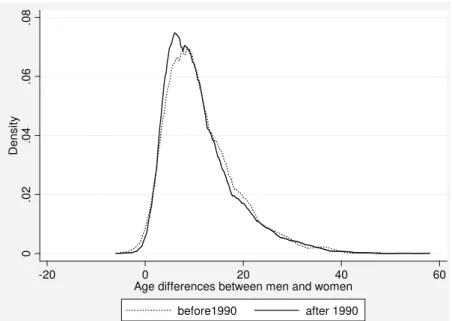
We restrict the sample to women who married when aged between 15 and 25 years old for two reasons. Firstly, most women get married in this age interval. In Lesotho, for instance, this sub-sample accounts for 90% of the total sample. Secondly, and more importantly, this sample restriction allows us to rule out heterogeneities in the marital pattern from our analysis. Indeed women who get married after reaching 25 years old might have been previously married to someone else, or might have different preferences in terms of partner selection compared to women who get married at younger age.
To obtain a first indicator as to whether the spread of AIDS in Africa has induced changes in the choice of partner, we draw the distribution of spousal age differences for a low-prevalence and a high-prevalence country and for two distinct samples: women who married before 1990 and those who married after 1990. Figure 1 charts the empirical distributions for Lesotho which is one of most affected countries in Sub-Saharan Africa since 23.6% of its adult population was HIV-infected in 2009 (UNAIDS, 2010). Similarly, Figure
2 charts the distributions for Niger, a country which has one of the lowest infection rates on the continent as its adult HIV prevalence rate reached 0.8% in 2009 (UNAIDS, 2010).
Figure 1, about here. Figure 2, about here.
Taking 1990 as a benchmark year, the two distributions are very similar, sug-gesting that there was no adjustment in behavior after populations became informed about the HIV/AIDS epidemic and its ways of transmission.
The Demographic and Health Surveys are standardized nationally rep-resentative household surveys that collect data in various African countries based on a standardized questionnaire. We are, thus, able to generalize our analysis by using a large set of countries3 in order to test whether the
distri-bution of the spousal age differences is constant over time.
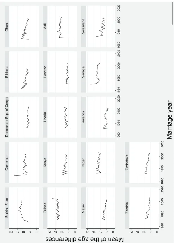
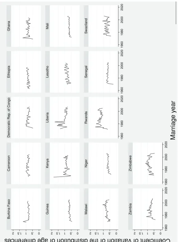
We use the survey to compute the mean and the coefficient of variation of the distribution of the spousal age differences by country and by marriage year. Figures 3 and 4 provide the dynamics of the mean and the coefficient of variation4, respectively, for each country of the sample.
Figure 3, about here. Figure 4, about here.
There is no clear pattern suggesting a change in the distribution of the age differences over time, except for Ghana and Malawi, where one could notice a downward trend in the mean from the mid-1980s onwards. The mean of age differences decreases from 1985 in Ghana and from 1986 in Malawi,
3The countries, with the date of the DHS survey, are the following: Burkina Faso
(2003), Cameroon (2004), Democratic Republic of Congo (2007), Ethiopia (2005), Ghana (2003), Guinea (2005), Kenya (2003), Lesotho (2004), Liberia (2007), Mali (2006), Malawi (2004), Niger (2006), Rwanda (2005), Senegal (2005), Swaziland (2006/07), Zambia (2007) and Zimbabwe (2005/06).
but these decreases are not statistically significant. If we go back to the individual data, and implement a T-test to test for the difference between the population mean of age differences in these years and at the end of the period, we find that in both cases, we cannot reject the null hypothesis that the population mean is equal in 1985 and in 2003 in Ghana (and in 1986 and in 2005 for Malawi).
To test the stability of the distribution of spousal age differences over time, we use a linear fixed effects model to successively estimate the mean and the coefficient of variation of the spousal age differences at the country-year level using as independent variables the marriage country-year and a dummy variable that takes value one if the marriage was celebrated before 1990 and zero otherwise. Empirical results presented in Table 1 suggest that the marriage year and the act of getting married before the spread of the AIDS epidemic have no statistically significant effect on the dependent variables, i.e. the mean (column 1) and the coefficient of variation (column 2).
Dependent variable mean coefficient of variation Marriage year −0.0311 (0.021) 0.0021 (0.002) 1 if marriage before 1990 0.0234 (0.244) 0.0467 (0.027) Constant 70.6746 (41.161) −3.315 (3.198)
Country effects Yes Yes
Number of observations 604 600
Number of countries 17 17 Table 1
Linear fixed effects estimates
(in parentheses: robust standard errors, clustered at the country level)
These stylized facts suggest that controlling for country-specific effects, distributions of spousal age differences are stable over time and that the onset of the epidemic disease does not imply any adjustment in preferences regard-ing the age difference between spouses. Therefore, grounded on this empirical
evidence, the next section will consider the dispersion of age differences as an exogenous parameter of the model.
3
Model
3.1
Basic setting
Our model can be seen as an extension of the model developed by Feng et al. (2005), which describes the spread of an epidemic disease in a multi-group model. Multi-multi-group modeling, comes for us, in the gender specific variables we use. Our main departure from the work of these authors lies in the definition of the boundary conditions that characterize the birth process. Indeed, we assume that the latter depends on sexual behaviors and that, as a consequence, it is intrinsically linked to the spread of the epidemic disease. Let Sg(t, a)and Ig(t, a)denote, respectively, the density at time t ∈ R+of
susceptible and infective individuals of age a ∈ [0, ω] and gender g ∈ {f, m} , where ω > 0 is the maximal length of life, and where f corresponds to the population of women and m to the population of men. Their dynamics are given by the following system of equations:
∂Sg(t, a)
∂t +
∂Sg(t, a)
∂a = −Sg(t, a) [μ (a) + λg(t, a)] , (1) ∂Ig(t, a)
∂t +
∂Ig(t, a)
∂a = −Ig(t, a) [μ (a) + μ1(a)] + Sg(t, a) λg(t, a) ,(2) where μ (a) and μ1(a) are, respectively, the mortality rate of individuals at age a and the over-mortality rate of infected individuals at age a. The probability of an individual of gender g and age a being infected at time t, the so-called force of infection denoted by λg(t, a), will be characterized
below.
Let Ng(t, a) = Sg(t, a) + Ig(t, a) denote the density of individuals of
gender g and age a at time t. Using (1) and (2), we obtain: ∂Ng(t, a)
∂t +
∂Ng(t, a)
The per head variables are defined as: sg(t, a) = Sg(t, a) Ng(t, a) and ig(t, a) = Ig(t, a) Ng(t, a) .
One important feature of our model is that the probability of being in-fected depends on the age of the partner, denoted a0. The minimum age at
which individuals become sexually active is denoted a0 ∈ [0, ω). We suppose
that the force of infection is given by: λg(t, a) =
Z ω a0
βg(a, a0) ρg(a, a0) i−g(t, a0) da0. (4) Note that the probability of being infected has three components. The com-ponent that will be crucial for our analysis is denoted by ρg(a, a0) and
rep-resents the average number of partners of age a0 and of opposite gender −g
per individual of age a and gender g (see Iannelli, 1995; Yang and Milner, 2009). We will below specify this function as a product of three factors and make its various components explicit. Two notable features are to be high-lighted here. On one hand, unlike Anderson et al. (1992), we assume that function ρg(a, a0) is time-independent. The assumption is crucial to derive
the theoretical results we present in this section. Our numerical simulations, presented in Section 4, suggest that allowing for time dependence barely af-fects the quantitative results. On the other hand, homosexual relationships are not considered in our model. The function βg(a, a0) is the
infectious-ness of the disease, i.e. the probability of being infected when having an infected partner of age a0. For most of the results that will be derived below,
we will keep this function general and dependent on the ages of both part-ners. Lastly, the force of infection depends on i−g(t, a0), the proportion of infectious individuals among those of age a0 and gender −g.
Let us now describe the boundary conditions that characterize the birth process. Let b (a) be the probability at age a of susceptible and infected women who have a sexual partner giving birth to a child. Furthermore, in order to simplify the model, assume that there is no vertical transmission of
the disease (i.e. all children are born susceptible). The boundary conditions are: ⎧ ⎨ ⎩ Sg(t, 0) = σg Rω 0 b (a) Nf(t, a) Rω a0ρf(a, a 0) da0da, Ig(t, 0) = 0,
where σg is the secondary sex ratio that satisfies σg[Nf(t, 0) + Nm(t, 0)] =
Ng(t, 0). Unlike Feng et al. (2005), we thus assume that birth depends on
contact behavior, which is the same as the one involved in the transmission of the disease, and that there is no vertical transmission. The initial conditions
are: ⎧ ⎨ ⎩ Sg(0, a) = Sg0(a) , Ig(0, a) = Ig0(a) , with S0
g(a) , Ig0(a) ∈ L1(0, ω) and Sg0(a) , Ig0(a) ≥ 0 a.e. in [0, ω]. In
summary, the system that is studied reduces to: ⎧ ⎪ ⎪ ⎪ ⎪ ⎨ ⎪ ⎪ ⎪ ⎪ ⎩ ∂ig(t,a) ∂t + ∂ig(t,a)
∂a = (1− ig(t, a)) [λg(t, a)− μ1(a)ig(t, a)] t > 0, a∈ (0, ω)
ig(t, 0) = 0 g ∈ {m, f},
ig(0, .) = i0g(.)∈ L1(0, ω; R+) g ∈ {m, f}.
(5) Because of the biological definition of ig, we introduce the following state
Banach lattice spaces X = L1
(0, ω; R) × L1
(0, ω; R) endowed together with the usual product norm. We also consider
C = ½µ if im ¶ ∈ X : 0 ≤ ig ≤ 1 a.e. g ∈ {f, m} ¾ . (6)
Finally, let us assume:
Assumption 1 Assume that μ1 ∈ L∞+ (0, ω; R+) and, for each g ∈ {f, m},
System (5) can hence be re-written as follows: ⎧ ⎪ ⎪ ⎪ ⎪ ⎪ ⎪ ⎪ ⎨ ⎪ ⎪ ⎪ ⎪ ⎪ ⎪ ⎪ ⎩ ∂ig(t,a) ∂t + ∂ig(t,a)
∂a = (1− ig(t, a)) [Λg[i−g(t, .)](a)− μ1(a)ig(t, a)] ,
ig(t, 0) = 0, ∀g ∈ {m, f}, Ã if(0, .) im(0, .) ! = Ã i0f (.) i0m(.) ! ∈ C, (7)
wherein we have set for each g ∈ {f, m}, the bounded linear operator Λg :
L1 (0, ω; R) → L∞(0, ω; R) defined as follows Λg[ϕ](.) = Z ω 0 γg(., a0)ϕ(a0)da0, ∀ϕ ∈ L1(0, ω; R),
where functions γg ≡ γg(a, a0) stand for the so-called rate of infection from
contacts between an infective individual of age a0 and a susceptible individual of age a (see Li and Brauer, 2008) such that
γg(a, a0) = βg(a, a0) ρg(a, a0) .
3.2
Local properties of the disease-free equilibrium
This section aims at deriving some basic mathematical properties of (7). The local dynamics are studied by analyzing the spectral radius of a linear operator of a related system. The difficulty comes from the fact that in contrast to most papers in the literature, we do not assume the separability of function γg(a, a0). It is therefore not possible to derive an explicit expressionfor the spectral radius. Spectral theory provides however well-known tools to obtain properties for the spectral radius. We establish some of its properties that will allow us, in the last part, to obtain some properties about the dynamics for specified contact rate functions.
The functional framework is defined as follows. Let us recall first that X = L1
(0, ω; R) × L1
(0, ω; R) is a Banach Lattice partially ordered with its positive cone X+ defined by
Moreover following the standard notion, for each (ϕ, ψ) ∈ X, the symbol ϕ≤ ψ means that ψ − ϕ ∈ X+.
Our first Lemma establishes the existence of a weak solution of system (7). Let α > 0 be given such that
α > μ1(a) + Λg[1](a), g∈ {f, m}, a.e. a ∈ (0, ω). (8)
Then, consider the linear operator A : D(A) ⊂ X → X defined by D(A) = ⎧ ⎨ ⎩ϕ = ⎛ ⎝ϕf ϕm ⎞ ⎠ ∈ W1,1 (0, ω; R)2 : ϕ (0) = (0, 0) ⎫ ⎬ ⎭, and A ⎛ ⎝ϕf ϕm ⎞ ⎠ = ⎛ ⎝−ϕ 0 f −ϕ0 m ⎞ ⎠ , and the nonlinear operator F : C → X defined by
F ⎛ ⎝ϕf ϕm ⎞ ⎠ = ⎛ ⎝ ¡ 1− ϕf¢ ¡Λf[ϕm]− μ1(a)ϕf ¢ (1− ϕm)¡Λm[ϕf]− ϕm ¢ ⎞ ⎠ .
Then, using u(t) = (if(t, .), im(t, .)), the system (7) can be rewritten as the
following abstract Cauchy problem: ⎧ ⎨ ⎩ du(t) dt = Au (t) + F (u (t)) , t > 0 u (0) = ϕ∈ C. (9)
Note that given the choice of α, for each (ϕ, ψ) ∈ C2
such that ϕ ≤ ψ, one obtains that:
F (ϕ) + αϕ≤ F (ψ) + αψ. Consequently, system (9) is equivalent to
⎧ ⎨ ⎩ du(t) dt = (A− α) u (t) + (F + α) (u (t)) , t > 0 u (0) = ϕ∈ C. (10)
Lemma 1. Let Assumption 1 be satisfied. Then, the operator (A, D(A)) is the infinitesimal generator of a C0−positive semigroup {TA(t)}t≥0 on X.
There exists a unique strongly continuous semiflow {U(t; . ) : C → C}t≥0
such that for each ϕ ∈ C, the map t → U(t; ϕ) is a mild solution of system (9), that is
U (t; ϕ) = TA(t)ϕ +
Z t 0
TA(t− s)F (U(s; ϕ) ds, ∀t ≥ 0.
Moreover for each (ϕ, ψ) ∈ C2 one has
ϕ≤ ψ, ⇒ U (t; ϕ) ≤ U (t; ψ) , ∀t ≥ 0.
Proof. The proofs of similar results can be found in Webb (1985), Busenberg et al. (1991) and Feng et al. (2005). A key ingredient is given by the positivity of the semigroup generated by A, namely
TA(t)ϕ(a) = ⎧ ⎨ ⎩ ϕ(a− t) if t < a 0 if t > a , ∀ϕ ∈ X. ¤
Let us now study the local dynamics in the neighborhood of the so-called disease free equilibrium (DFE, hereafter) that corresponds to the station-ary solution: IDF E = ¡iDF E
f , iDF Em
¢
= (0, 0) of (7). The DFE satisfies Ig(t, a) ≡ 0, implying that Sg(t, a) = Ng(t, a) , where Ng(t, a) solves the
classical Lotka-McKendrick equation given by: ⎧ ⎪ ⎪ ⎪ ⎪ ⎨ ⎪ ⎪ ⎪ ⎪ ⎩ ∂Ng(t,a) ∂t + ∂Ng(t,a) ∂a =−μ (a) Ng(t, a) , Ng(t, 0) = σg Rω 0 b (a) Nf(t, a) Rω a0ρf(a, a 0) da0da, Ng(0, a) = Ng0(a) g ∈ {m, f}. (11)
Remark 1. Textbooks like Webb (1984) and Iannelli (1995) can be used to prove the existence of a DFE with intrinsic growth rate λ characterized by:
1 = σf Z ω 0 b (a) e−U0a(μ(z)+λ)dz Z ω a0 ρf(a, a0) da0da,
with densities for men and women given by: Ng∗(t, a) = e λt Ng0e− Ua 0(μ(z)+λ)dz,
where the Ng0 can be computed easily.
We now aim at proving that the linear stability of the DFE is related to the so-called basic reproduction number. The corresponding linearized equation around the DFE is given by:
∂uf(t, a)
∂t +
∂uf(t, a)
∂a =−μ1(a) uf + Λf[um(t, .)](a), ∂um(t, a)
∂t +
∂um(t, a)
∂a =−μ1(a) um+ Λm[uf(t, .)](a),
(12) and uf(t, 0) = um(t, 0) = 0, (uf, um) (0, .) = ¡ u0f, u0m ¢ ∈ X. (13)
In order to study this linear equation, we consider linear operator bA : D³Ab´⊂ X → X and bounded linear operator B : X ⊂ X → X defined by
D³Ab´= D(A), A =b µ −dad − μ1(a) 0 0 −dad − μ1(a) ¶ , and B = µ 0 Λf Λm 0 ¶ .
Then, by setting u(t) = (uf(t, .), um(t, .)), system (12)-(13) can be written as
follows: du(t) dt = ³ b A + B´u(t), t > 0, u(0) = u0 = µ u0 f u0 m ¶ ∈ X.
In order to study some properties of the above linear problem, let us first establish the following result:
Theorem 1. Linear operator bA + B : D(A)⊂ X → X is the infinitesimal generator of positive C0−semigroups {TA+Be (t)}t≥0 on X. We also have the
fixed-point formulation: T( eA+B)(t) = TAe(t) + Z t 0 BTA+Be (s)ds, ∀t ≥ 0, and ωess( bA + B) =−∞, ω0( bA + B) = s( bA + B)∈ σ ³ b A + B ´ . (14) Here, ωess( bA + B) denotes the essential growth rate of {T( eA+B)(t)}t≥0, while
ω0( bA + B) and s( bA + B) respectively denote the growth rate of TA+Be (t) and
the spectral bound of ( bA + B). Proof. It is easy to see that
TAe(t)ϕ = ⎧ ⎨ ⎩ 0 if t > a e−Uaa−tμ1(s)dsϕ(a− t) if a > t.
This proves that TAe(t)is a nilpotent semigroup and therefore, we obtain that ωess
³ b A ´
=−∞. To prove the other part of (14), we need to prove that for each t > 0, the operator BTAe(t)B is weakly compact in X. Recalling that TAe(t) = 0 for all t ≥ ω, it is sufficient to consider the case t ∈ (0, ω). Let t ∈ (0, ω) be given. Then, we have:
BTAe(t)B = µ C1 0 0 C2 ¶ , wherein we have set
C1ϕf = Z ω 0 daγ(a, .)1(t,ω)(a)e− Ua a−tμ(s)ds Z ω 0 γm(a− t, a0)ϕf(a0)da0 C2ϕm = Z ω 0
daγm(a, .)1(t,ω)(a)e− Ua
a−tμ(s)ds
Z ω 0
γf(a− t, a0) ϕm(a0) da0. Note that operators C1 and C2 both act on L1(0, ω) and are bounded linear
operators. Moreover, they satisfy 0≤ Ciϕ≤ M
Z ω 0
ϕ(s)ds, ∀ϕ ∈ L1+(0, ω),
for some constant M > 0 independent of ϕ. We conclude that C1 and C2 are
both weakly compact operators, and thus BTA(t)B is also weakly compact.
Before establishing the local stability of the DFE, let us propose a formal definition of the basic reproduction number and make a remark.
Definition 1 (Basic reproduction number). Consider the bounded linear operator T0 ∈ L(X) defined by T0 =
³
− bA´−1B and define the following quantity
R0 = r (T0) .
Remark 2. One has the following explicit expression for operator T T0ϕ =
Z ω 0
G0(., u)ϕ(u)du, ∀ϕ ∈ X,
wherein we have set: G0(a, u) = Z a 0 e−Ua0aμ1(s)ds µ 0 γf(a0, u) γm(a0, u) 0 ¶ da0.
The next Theorem establishes the local stability of the DFE.
Theorem 2. Let Assumption 1 be satisfied. The disease free equilibrium is locally asymptotically stable if R0 < 1, and is unstable if R0 > 1.
To prove Theorem 2, we demonstrate two Lemma. We first notice that due to Theorem 1, the local stability of the DFE is related to the location of the real value s³A + Bb ´ with respect to zero. Consider for each λ ∈ R the bounded linear operator Tλ : X → X defined by:
Tλ µ ϕf(a) ϕm(a) ¶ = Z ω 0 Gλ(a, u) µ ϕf(u) ϕm(u) ¶ du, where Gλ(a, u) = Z a 0 e−(a−a0)λ−Ua0aμ1(s)ds µ 0 γf(a0, u) γm(a0, u) 0 ¶ da0. Then, one has the following Lemma.
Lemma 2. For each λ ∈ R, the operator Tλ is positive and compact.
More-over, for each λ ≤ λ0, one has:
Tλ0ϕ≤ Tλϕ, ∀ϕ ∈ X+.
Proof. The positiveness is obvious as well as the decreasing property with respect to λ. The compactness follows by noticing that for each λ ∈ R, operator Tλ is regularizing in the sense that it maps the unit ball of X into
a bounded set of W1,∞(0, ω; R2). ¤
Next, consider the map R : R → [0, ∞) defined by R(λ) = r (Tλ) , ∀λ ∈ R,
wherein for each L ∈ L(X), the quantity r (L) denotes the spectral radius of L. Then, we obtain the following result.
Lemma 3. Let Assumption 1 be satisfied. Then, the map λ 7→ R(λ) is continuous, decreasing and satisfies
lim
λ→∞R(λ) = 0,
R(0) = R0 (see Definition 1) and R(s) = 1 where s := s
³ b A + B
´
denotes the spectral bound of operator bA + B.
Proof. Let us first notice that the map λ 7→ Tλ is continuous from R to
L(X). Since Tλ is compact for each λ ∈ R, we conclude that λ 7→ R(λ)
is continuous. As a consequence, due to Lemma 2, the map λ 7→ R(λ) is decreasing. Then, it is easy to check that
lim
λ→∞kTλkL(X) = 0,
which implies that R(λ) → 0 when λ → ∞. It is also easy to check that λ ∈ R ∩ σp
³ b
wherein σp denotes the point spectrum. From this and the positivity, it
follows that R(s) = 1. ¤
A direct consequence of Lemma 3, is that if R0 < 1,then s = s
³ b
A + B´< 0 and if R0 > 1, then s > 0. This completes the proof of Theorem 2.
Theorem 3. Let Assumption 1 be satisfied. If R0 > 1, then system (7) has
at least one endemic stationary state, i.e. there exist (ief, iem)∈ C∩D(A)\{0}
such that: ⎧ ⎨ ⎩ die g(a) da = ¡ 1− ie g(a) ¢ £
Λg[ie−g](a)− μ1(a)ieg(a)
¤ , ie
g(0) = 0, ∀g ∈ {m, f}.
Proof. Let us recall that as R0 > 1, there exists λ > 0 such that R(λ) = 1.
Let ϕ = µ
ϕf ϕm
∈ X+ be given such that T
λϕ = ϕ.Consider now the
follow-ing fixed point problem: find u ∈ C\{0} such that u = ³− bA− α´−1(F + α) u. Since the operator ³− bA− α´−1 is positive and F is increasing, one obtains by setting e = (1, 1) that
³
− bA− α´−1(F + α) e≤³− bA− α´−1αe≤ e. On the other hand, for each ε > 0 one has
³ − bA− α´−1(F + α) [εϕ](a) = ε Z a 0 eα(t−a) µ¡ 1− εϕf(t) ¢ ¡ Λf[ϕm]− μ1(a)ϕf ¢ + αϕf (1− εϕm) ¡ Λm[ϕf]− μ1(t)ϕm ¢ + αϕm. ¶ dt = ε Z a 0 eα(t−a) µ Λf[ϕm]− μ1(a)ϕf + αϕf − εϕf ¡ Λf[ϕm]− μ1(a)ϕf ¢ Λm[ϕf]− μ1(t)ϕm+ αϕm− εϕf(t) ¡ Λf[ϕm]− μ1(a)ϕf ¢ ¶ dt This implies that:
³ − bA− α ´−1 (F + α) [εϕ](a) = εϕ(a) + ε Z a 0 eα(t−a) µ ϕf(t)¡λ− ε¡Λf[ϕm]− μ1(a)ϕf ¢¢ ϕm¡λ− ε¡Λf[ϕf]− μ1(a)ϕm ¢¢ ¶dt.
As a consequence, if ε > 0 is chosen small enough so that εϕ≤ e and ε µ Λf[ϕm]− μ1(a)ϕf Λf[ϕf]− μ1(a)ϕm ¶ ≤ λe, one obtains that
³
− bA− α´−1(F + α) [εϕ]≥ εϕ.
The above inequality allows us to start a monotone iterative procedure to get complete the proof of the result. ¤
Theorem 4. Assume that no nontrivial equilibrium exists. Then the fol-lowing holds true for each ϕ ∈ C:
U (t; ϕ)→ 0 as t → ∞.
Proof. Let ϕ ∈ C be given and set e = (1, 1)T ∈ C. Let us first notice that the map t 7→ U(t; e) is decreasing. Indeed for each t ≥ 0 one has U(t; e) ∈ C so that
U (t; e)≤ e.
Then since U is monotone, for each s ≥ 0, one gets that U (t + s; e)≤ U(s; e),
and the result follows. Therefore U (t; e) converges to some equilibrium point when t → ∞. Due to the assumption, this leads us to
U (t; e)→ 0 as t → ∞.
Finally since ϕ ≤ e, due to the monotony, one gets that U (t; ϕ)≤ U(t; e), ∀t ≥ 0. ¤
3.3
Global properties of the disease-free equilibrium
Theorem 2 provided some local conditions about the stability of the DFE. We now aim at exhibiting a condition such that the DFE is unique, which allows for assessing its global stability. First of all, Lemma 4 provides a re-formulation of the equilibrium system of equations.Lemma 4. Let Assumption 1 be satisfied. Let u = (uf, um) be a non trivial
equilibrium of (7). Then, u satisfies
ug =F (Λg[u−g]) , g∈ {f, m}, where F is defined by F (ϕ) (a) = Ra 0 e Ut 0μ1(s)dsϕ(t)e− Ut 0ϕ(s)dsdt eU0aμ1(s)dse− Ua 0 ϕ(s)ds+Ra 0 e Ut 0μ1(s)dsϕ(t)e− Ut 0ϕ(s)dsdt .
Proof. The proof of this lemma is related to the well known quadrature for-mula for the logistic equation. If one considers the non-autonomous logistic equation:
u0(t) = u(t) (a(t)− b(t)u(t)) , u(0) = x0 > 0,
then the solution is given by
u(t) = exp³R0ta(τ )dτ´ 1 x0 + Rt 0 b(τ ) exp ¡Rτ 0 a(ξ)dξ ¢. The re-formulation follows after some algebra. ¤
From this re-formulation, one can obtain the following result.
Theorem 5. Consider the linear bounded and positive operator bT : X → X defined by b T ϕ(a) = Z ω 0 b G(a, u)ϕ(u)du,
wherein we have set b G(a, u) = Z a 0 e−Utaμ1(s)ds µ 0 eUtaΛf[1](s)dsγ f(t, u)dt eUtaΛm[1](s)dsγ m(t, u) 0 ¶ dt.
If r³Tb´< 1, the only equilibrium of system (7) is the DFE.
Proof. Let u = (uf, um) be a nontrivial equilibrium of (7). If we set
ξ−g = Λg[u−g] then we obtain ug(a)≤ Z a 0 e−Utaμ1(s)dsξ −g(t)e Ua t ξ−g(s)dsdt. Thus ug(a)≤ Z a 0 e−Uta(μ1(s)−Λg(s))dsΛ g[u−g](t)dt.
As a consequence, one obtains that u ≤ bT u. This implies that r³Tb´ ≥ 1 and the result follows. ¤
Note that T0 ≤ bT so that R0 ≤ r
³ b
T´. As a consequence of the two results presented above, we obtain that when r³Tb´ < 1 then the disease free equilibrium is globally asymptotically stable. These results could be completed by a global analysis of endemic equilibrium. This task, however, is beyond the scope of this paper.
4
The impact of the dispersion of age
differ-ences between partners
In this section, we compute numerically the value of the epidemic threshold, R0, as a function of the mean and the variance of the distribution of age
differences between partners.
4.1
Parameters and functions of the model
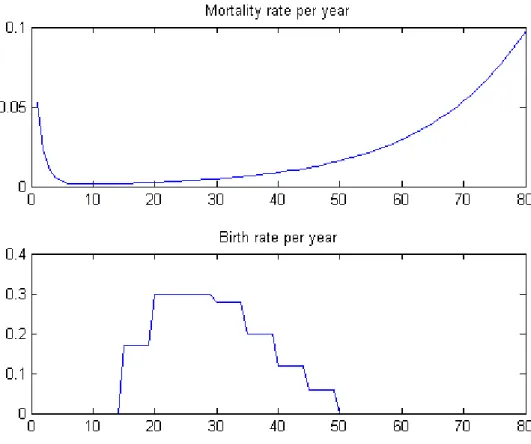
The model is simulated using parameters that are similar to those used in Anderson et al. (1992), including the age-specific mortality and fertility rates
displayed in Figure 5.
Figure 5, about here.
For mortality, which is supposed to be similar for men and women, we use the Siler approximation, and obtain that life expectancy at birth is 55.069 years. Concerning fertility, we obtain a Total Fertility Rate of 7.15. The demographic growth rate of the disease-free population can be computed using the formula given in Remark 1, and is equal to λ = 0.076. Concerning the epidemiological parameters, we suppose that the infectiousness of the disease is age-independent, βg(a, a0) = β
g and that a susceptible woman has
a risk of infection when having a sexual contact with an infected man which is three times higher than those involving a susceptible man and an infected woman. The over-mortality rate of infected individuals is also supposed to be age independent, μ1(a) = μ1, and has been set such that the life expectancy
(ignoring other causes of death) is 5 years. Parameters are given in Table 2.
Sex ratio at birth,σg 0.5
Maximal age at death,ω 80
Minimal age of sexual activity,a0 15
Lower and upper limits ages for fertility,a1 and a2 15and 50
Over-mortality rate,μ1 0.2
Infectiousness of the disease, βf and βm 0.3and 0.1 Table 2
Parameters of the simulated model
The main difficulty when simulating our model concerns the function describing the average number of partners. In Section 3, the average number of partners of age a0 and gender −g per individual of age a and gender g was characterized by a general time-independent function, ρg(a, a0). Time
independence was a necessary assumption in order to develop the theoretical analysis. In the present section, we relax this assumption and extend the analysis. Following Anderson et al. (1992), we allow for time-dependence for one gender and propose to decompose the function. Suppose that the average
number of partners can be represented by the product of two functions: cg(a, t), the rate of partner change for an individual of age a and gender
g at time t, and Jg(a, a0, t), a mixing function indicating, at time t, the
probability that an individual of age a and gender g chooses a partner of age a0. It satisfiesRa2
a1 Jg(a, a
0, t) da0 = 1. We hence have:
ρg(a, a0, t) = cg(a, t) Jg(a, a0, t) .
Functions cg(a, t) and Jg(a, a0, t) are linked to each other through the
fol-lowing constraint:
cf (a) Jf(a, a0) Nf(a, t) = cm(a0, t) Jm(a0, a, t) Nm(a0, t) (15)
Then, assume that, for women, the mixing function is given by:
Jf(a, a0) = ⎧ ⎪ ⎪ ⎪ ⎨ ⎪ ⎪ ⎪ ⎩ e− (a−a0+ν)2 2σ2 Ua2 a1 e −(a−α+ν)2 2σ2 dα for a, a0 ∈ [a1, a2] , 0 otherwise.
where ν > 0 stands for the mean age difference between men and women and σ > 0 for the standard deviation that measures the dispersion of age differences within couples. The function describing the mean rate of partner change comes from Anderson et al. (1992), so that:
cf(a) = ⎧ ⎨ ⎩ η for a ∈ [a1, a2] , 0otherwise.
The mean rate of partner change for men is given by: cm(a0, t) = Ra2 a1 cf(a) Jf(a, a 0) N f(a, t) da Nm(a0, t) ,
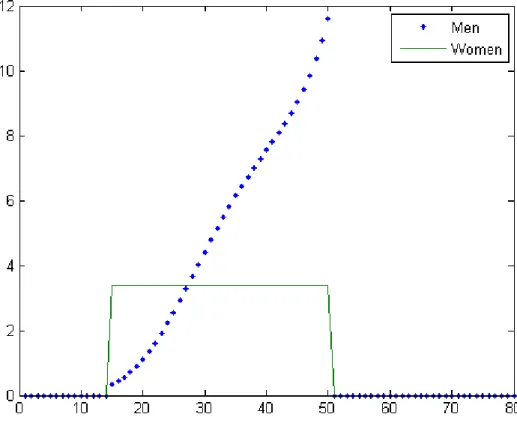
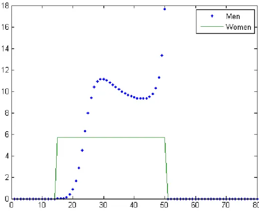
while the mixing function is computed according to (15). For instance, in the following figures, the mean rates of partner change per year as functions of age are pictured at the endemic equilibrium. We use the mean values of ν
and σ computed among our sample of African countries, namely ν = 8.78 and σ = 2.62. Concerning the parameter of function cf (a), we follow Anderson
et al. (1992) by using η = 3.4 and η = 5.7, as depicted in Figure 6 and Figure 7, respectively.
Figure 6, about here. Figure 7, about here.
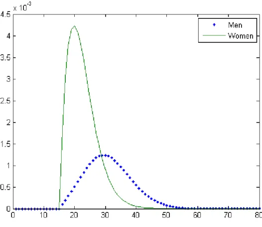
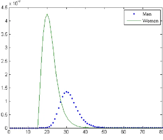
Similarly, we compute the average prevalence at the endemic equilibrium as well as the prevalence per age for men and women. Using η = 3.4 (Figure 8) and η = 5.7 (Figure 9), we obtain that the prevalence is equal to 1.5% and 5%, respectively.
Figure 8, about here. Figure 9, about here.
Two notable features of these figures are that (i) women are proportionally more infected than men and (ii) the mean age of the infected population is lower for women than for men. Both conclusions are consistent with empirical evidence found in previous studies (e.g. Buvé et al.; 2001, Glynn et al., 2001; Gouws et al., 2008; UNAIDS, 2010, chapter 2).
4.2
Numerical results
The aim of the numerical simulations is twofold. Firstly the numerical sim-ulations aim at evaluating the effect of both the mean and the variance of the age differences on the basic reproduction number. Secondly, it allows us to analyze the quantitative implication of assuming the time-independence of function ρ (a, a0), as we made in the previous section.
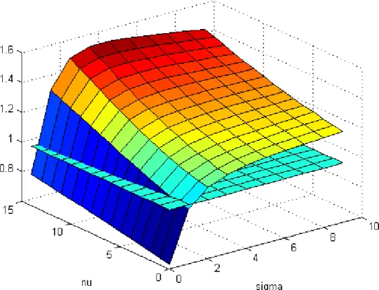
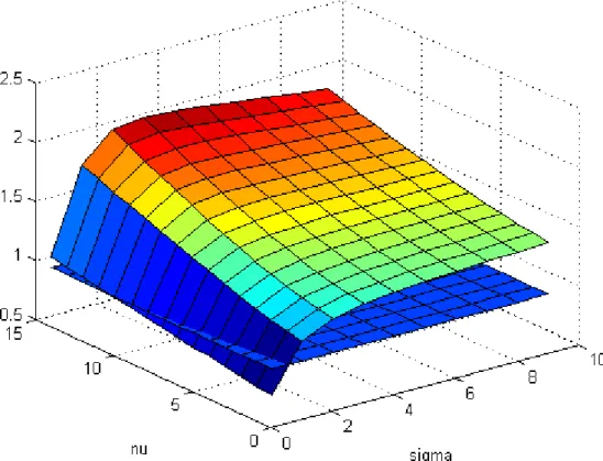
We compute the basic reproduction number as a function of the mean age difference, ν, and the standard deviation, σ using two different values of the parameter of function cf (a) used in Anderson et al. (1992): η = 3.4
figures clearly show that the epidemic threshold, R0, is an increasing function
of ν and an increasing and concave function of σ. The latter relationship becomes almost flat for values of σ greater than 3. Figure 10 shows that if the women’s rate of partner change is not too large, the standard deviation of age differences is a key parameter. Indeed, we find that if the standard deviation is small enough, the basic reproduction number remains below one whatever the value of the mean age difference. Conversely, if the standard deviation is large enough, the basic reproduction number is always greater than 1 even for very low mean age difference.
Figure 10, about here. Figure 11, about here.
In order to evaluate the impact of the assumption of time-independence of function ρ (a, a0), we compare the R0 computed by our model and those
computed by another model, for which the only difference lies in the way the function ρ (a, a0) is defined. Precisely, we consider an approximation of the
rate of partner change for men by assuming that μ1 is small and by using the stationary values of Nf(a, t) and Nm(a0, t) . With this approximation,
we obtain the following time independent functions: cm(a0) = Z a2 a1 cf (a) Jf(a, a0) e− Ua a0μ(u)+λduda, and Jm(a0, a) = cf(a) Jf (a, a0) e− Ua 0 μ(u)+λdu Ra2 a1 cf(α) Jf(α, a 0) e−U0αμ(u)+λdudα .
As a consequence, the kernel of λg is time independent. Figure 12 represents
the R0 as a function of σ for ν = 8.78 and η = 3.4 for both the initial model
and the approximated model.
We conclude that the approximation of the function ρ (a, a0, t) with a time
independent counterpart does not yield to notable quantitative differences, except that the approximation overestimates the R0.
5
Conclusion
In this paper, we have analyzed the effect of a change in the dispersion of age differences between sexual partners on the endemic nature of the HIV epidemic. Once we established empirically that the distribution of age dif-ferences in Sub-Saharan Africa had not been modified since the onset of the epidemic, we went on to create an age- and gender-structured dynamic model. We characterized the stability of the epidemic equilibrium and showed that variance plays a crucial role in the determination of the stability properties of this equilibrium. Moreover, the mean age difference has barely no impact on the stability of the disease-free equilibrium if the variance is sufficiently high.
Importantly, our model constitutes a tool in order to evaluate the impact of the two first moments of the age differences distribution on the asymptotic dynamics of the HIV epidemics. We show that a larger variance increases the likeliness that the disease-free equilibrium is unstable, and consequently that the epidemic is endemic. This is an asymptotic result that is not necessarily connected to the prevalence rate at a given point in time. It cannot be tested using past prevalence rates, be used to forecast the dynamics of HIV in the next few years in African countries and is not able to evaluate the various policies that have been launched in the countries of our sample. It rather argues that, everything equal, countries that have a large variance of age difference between partners should be particularly active in the fight against the spread of HIV within the population.
Moreover, in order to focus on the age differences, we have not considered other factors that may influence the dynamics of the epidemics. Our model
builds a framework suitable for incorporating other contextual features that could allow for more realism. Especially, our model may be extended by describing precisely the different variables that influence the contact function between generations. We have, indeed, concentrated on the probabilities of having some infectious contacts for an exogenous number of contacts per age. Since this number appears to be important, we must seek to understand the underlying behaviors, which would be a promising avenue of research.
References
[1] Anderson, R. M., May, R. M., Ng, T. W., and Rowley, J. T. (1992). Age-dependent choice of sexual partner and the transmission dynamics of HIV in Sub-Saharan Africa. Philosophical Transactions of the Royal Society B, 336: 135-185.
[2] Auvert B., Buvé A., Ferry B., Caraël M., Morison L., Lagarde E., Robin-son N.J., Kahindo M., Chege J., Rutenberg N., MuRobin-sonda R., Laourou M., Akam E. and Study Group on the Heterogeneity of HIV Epidemics in African Cities (2001). Ecological and individual level analysis of risk factors for HIV infection in four urban populations in sub-Saharan Africa with different levels of HIV infection. AIDS, 15 (supp 4): S15-S30. [3] Bergstrom, T. and Lam, D. (1994). The Effects of Cohort Size on
Marriage-Markets in Twentieth-Century Sweden. In J. Ermisch and N. Ogawa (Eds): The Family, the Market, and the State in Ageing Soci-eties. Oxford, UK: Clarendon Press. Reprint No. 454.
[4] Blanc, A.K., and Wolff, B. (2001). Gender and decision-making over condom use in two districts in Uganda. African Journal of Reproductive Health, 5 (3): 15-28.
[5] Boerma, J. T., Gregson, S., Nyamukapa, C., Urassa, M. (2003). Under-standing the uneven spread of HIV within Africa: Comparative study of biologic, behavioral, and contextual factors in rural populations in Tan-zania and Zimbabwe. Sexually Transmitted Diseases 30 (10): 779-787. [6] Brouard, N. (1994). Aspects démographiques et conséquences de
l’épidémie de sida. In J. Vallin (Ed.), Population Africaines et Sida. Paris: La Découverte, 119-178.
[7] Busenberg, S. N., Iannelli, M., and Thieme, H. R. (1991). Global be-havior of an age-structured epidemic model. SIAM J. on Mathematical Analysis, 22 (4): 1065-1080.
[8] Buvé A., Caraël M., Hayes R.J., Auvert B., Ferry B., Robinson N.J., Anagonou S., Kanhonou L., Laourou M., Abega S., Akam E., Zekeng L., Chege J., Kahindo M., Rutenberg N., Kaona F., Musonda R., Sukwa T., Morison L., Weiss H.A., Laga M. and Study Group on Heterogeneity of HIV Epidemics in African Cities (2001). Multicentre study on factors determining differences in rate of spread of HIV in sub-Saharan Africa: methods and prevalence of HIV infection. AIDS, 15 (supp 4), S5-S14.
[9] Casterline, J., Williams, L., and McDonald, P., (1986). The age differ-ence between spouses: Variations among developing countries. Popula-tion Studies, 40 (3): 353-374.
[10] Clément, Ph., Heimans, H. J. A. M., Angenent, S., van Duijn, C. J., and de Pagter, B. (1987). One-Parameter Semigroups, CWI Monographs 5, Amsterdam: North-Holland.
[11] Feng, Z., Huang, W., and Castillo-Chavez, C. (2005). Global behav-ior of a multi-group SIS epidemic model with age structure. Journal of Differential Equations, 218(2): 292-324.
[12] Glynn, J. R., M. Carael, B. Auvert, M. Kahindo, J. Chege, R. Musonda, F. Kaona, and Buve, A. (2001). Why do young women have a much higher prevalence of HIV than young men? A study in Kisumu, Kenya and Ndola, Zambia. AIDS, 15(S4): S51—S60.
[13] Gregson, S., Nyamukapa, C., Garnett, G., Mason, P., Zhuwau, T., Caraël, M., Chandiwana, S., and Anderson, R. (2002). Sexual mixing patterns and sex-differentials in teenage exposure to HIV infection in rural Zimbabwe. Lancet, 359: 1896—1903.
[14] Grobler, J. J. (1987). A note on the theorems of Jentzsch-Perron and Frobenius. Indagationes Mathematicae (Proceedings), 90 (4): 381—391. [15] Grobler, J. J. (1995). Spectral Theory in Banach Lattice. In C.B.
Hui-jsmans, M.A. Kaashoek, W.A.J. Luxemburg, and B. de Pagter (Eds.): Operator Theory in Function Spaces and Banach Lattice (Operator The-ory, Advances and Applications 75). Bassel: Birkhauser, 133-172. [16] Gouws, E. Stanecki, K., Lyerla, R., and Ghys, P. (2008). The
epidemiol-ogy of HIV infection among young people aged 15—24 years in southern Africa. AIDS, 22 (suppl 4), S5—S16.
[17] Iannelli, M. (1995). Mathematical theory of age-structured population dynamics, Applied Mathematics Monographs 7. Pisa: Giardini editori e stampatori.
[18] Kelly, R.J., Gray, R.H., Sewankambo, N., Serwadda, D., Wabwire-Mangen, F., Lutalo, T., and Wawer, M.J., (2003). Age Differences in Sexual Partners and Risk of HIV-1 Infection in Rural Uganda. Journal of Acquired Immune Deficiency Syndromes, 32 (4): 446-451.
[19] Konde-Lule, JK., Sewankambob, N., and Morris, M., (1997). Adoles-cent sexual networking and HIV transmission in rural Uganda. Health Transition Review, 7 (supplement): 89-100.
[20] Li, J., and Brauer, F. (2008). Continuous-time age-structured models in population dynamics and epidemiology. In F. Brauer, P. van den Driessche, and J. Wu (Eds.): Mathematical Epidemiology, Lecture Notes in Mathematics 1945. Berlin: Springer, 205-227.
[21] Luke, N. (2003). Age and economic asymmetries in the sexual relation-ships of adolescent girls in Sub-Saharan Africa. Studies in Family Plan-ning, 34 (2): 67-86.
[22] Luke, N. (2005). Confronting the ‘Sugar Daddy’ stereotype: Age and economic asymmetries and risky sexual behavior in urban Kenya. Inter-national Family Planning Perspectives, 31 (1): 6-14.
[23] Marek, I. (1970). Frobenius theory of positve operators: Comparison theorems and applications, SIAM Journal on Applied Mathematics, 19 (3): 607-628.
[24] Meyer-Nieberg, P. (1991). Banach Lattices. Berlin: Springer-Verlag. [25] Schaefer, H. (1974). Banach Lattices and Positive Operators. New-York:
Springer-Verlag.
[26] Spijker, J.J.A. (2011). Worldwide household patterns of young couples in multilevel perspective. Brown Bag Seminar presentation to the Survey Research Center and Population Studies Center, University of Michigan, Ann Arbor, 03/29/2011.
[27] UNAIDS (2010). Global report: UNAIDS report on the global AIDS epidemic 2010, UNAIDS/WHO.
[28] Webb, G. F. (1984). A semigroup proof of the Sharpe Lotka theorem. Lecture Notes in Mathematics 1076. Berlin: Springer, 254-268.
[29] Webb, G. F. (1985). Theory of Nonlinear Age-Dependent Population Dynamics. New York: Marcel Dekker.
[30] Yang, K. and Milner, F. (2009). The logistic, two-sex, age-structured population model. Journal of Biological Dynamics, 3 (2-3): 252-270. [31] Zerner, M. (1987). Quelques propriétés spectrales des opérateurs positifs.
0 .0 5 .1 .1 5 D e n s it y -20 0 20 40 60
Age differences between men and women
before1990 after 1990
Figure 1: Distribution of age differences between men and women at marriage for Lesotho 0 .0 2 .0 4 .0 6 .0 8 D e n s it y -20 0 20 40 60
Age differences between men and women
before1990 after 1990
Figure 2: Distribution of age differences between men and women at marriage for Niger
0 5 10 15 20 20 15 10 5 0 20 15 10 5 0 20 15 10 5 0 1 9 6 0 1 9 8 0 2 0 0 0 2 0 2 0 1 9 6 0 1 9 8 0 2 0 0 0 2 0 2 0 1 9 6 0 1 9 8 0 2 0 0 0 2 0 2 0 1 9 6 0 1 9 8 0 2 0 0 0 2 0 2 0 1 9 6 0 1 9 8 0 2 0 0 0 2 0 2 0 B u rk in a F a s o C a m e ro o n D e m o c ra ti c R e p . o f C o n g o E th io p ia G h a n a G u in e a K e n y a L ib e ri a L e s o th o M a li M a la w i N ig e r R w a n d a S e n e g a l S w a z ila n d Z a m b ia Z im b a b w e
Me
an
o
f t
he
a
ge
d
iff
ere
nc
es
M
a
rr
ia
g
e
y
e
a
r
0 .5 1 1.5 2 2 1.5 1 .5 0 2 1.5 1 .5 0 2 1.5 1 .5 0 1 9 6 0 1 9 8 0 2 0 0 0 2 0 2 0 1 9 6 0 1 9 8 0 2 0 0 0 2 0 2 0 1 9 6 0 1 9 8 0 2 0 0 0 2 0 2 0 1 9 6 0 1 9 8 0 2 0 0 0 2 0 2 0 1 9 6 0 1 9 8 0 2 0 0 0 2 0 2 0 B u rk in a F a s o C a m e ro o n D e m o c ra ti c R e p . o f C o n g o E th io p ia G h a n a G u in e a K e n y a L ib e ri a L e s o th o M a li M a la w i N ig e r R w a n d a S e n e g a l S w a z ila n d Z a m b ia Z im b a b w e
Co
eff
ic
ie
nt
of
va
ria
tio
n o
f t
he
d
is
tri
bu
tio
n o
f a
ge
d
iff
ere
nc
es
M
a
rr
ia
g
e
y
e
a
r
Figure 5: Mortality and fecondity as functions of age
Figure 6: Mean rate of partner change as a function of age for η = 3.4
Figure 7: Mean rate of partner change as a function of age for η = 5.7
Figure 8: Prevalence rate as a function of age for η = 3.4
Figure 9: Prevalence rate as a function of age for η = 5.7
Figure 10: R0 as a function of ν and σ for η = 3.4
Figure 11: R0 as a function of ν and σ for η = 5.7
Figure 12: R0 as a function of σ for the initial model and the approximated one