A NEW COMPREHENSIVE APPROACH
FOR BONE REMODELING UNDER MEDIUM AND HIGH MECHANICAL LOAD BASED ON CELLULAR ACTIVITY DANIELGEORGE, RACHELEALLENA, CÉLINEBOURZAC, STÉPHANEPALLU,
MORADBENSIDHOUM, HUGUESPORTIER AND YVESRÉMOND
Most of the last century, bone remodeling models have been proposed based on the observation that bone density is dependent on the intensity of the applied me-chanical loads. Most of these cortical or trabecular bone remodeling models are related to the osteocyte mechanosensitivity, and they all have a direct correlation between the bone mineral density and the mechanical strain energy. However, ex-periments on human athletes show that high-intensity sport activity tends not to in-crease bone mineral density but rather has a negative impact. Therefore, it appears that the optimum bone mineral density would develop for “medium”-intensity activity (or medium mechanical loads) and not for the highest-intensity one.
In this work, we propose a new continuum approach based on bone cell activ-ity being either positive or negative as a function of the intensity of the applied mechanical load. At standard earth gravity without exercise, bone homeostasis is observed with cell
activity being at equilibrium. When “medium loads” such as
“low-intensity” or “optimized” sport activity are applied, cells are activated and an increase of bone density occurs. On the other hand, “high-intensity loads” such as over-training lead to bone density decrease or bone degradation. Our results are in agreement with the literature and enable us to foresee applications such as optimal sport training for best physical conditions.
1. Introduction
The last hundred years or so have seen many bone remodeling models being devel-oped under the hypothesis that the mechanical energy is the main driving parameter of this complex phenomenon. According to the first law of bone remodeling de-fined in [Wolff 1986] and reprinted many times, bone mineral density is directly
Communicated by Emilio Barchiesi. George and Allena share first-authorship. 65Z05, 92C05
Keywords: bone remodeling, cellular activity, high and medium mechanical loads, osteoblasts, osteoclasts.
dependent on the intensity of the applied mechanical loads. Many strain-related models for bone remodeling have followed since. To name a few, see for exam-ple [Carter 1984], [Frost 1987] and its “mechanostat” proposal, [Cowin 1986], [Beaupré et al. 1990],[Turner 1998], or more recently [Lekszycki 2002] where the highly heterogeneous bone microstructure is seen as an optimum structural response to given external mechanical boundary conditions. Many theoretical frameworks of bone remodeling were proposed for cortical [Pivonka et al. 2008] and trabecular [Ruimerman et al. 2005] bone accounting for different bone cells at the origin of this remodeling [Pivonka and Komarova 2010;Klein-Nulend et al. 2013]. More recently, further theoretical models were proposed [Madeo et al. 2011; 2012;Lekszycki and dell’Isola 2012;Scala et al. 2017], some of them also taking into account the complex viscous mechanical behavior of the bone [Andreaus et al. 2014b;Giorgio et al. 2016;2017].
Nowadays, it is generally accepted that without considering the specific effects of the bone cells, whatever the theoretical model, the prediction of bone remodeling remains at best phenomenologically driven. Although at the continuous level (scale of the bone) the continuum mechanics is “manageable”, the integration of contin-uum biology is highly risky since, for the time being, there are no experimental measurements available in the literature able to link the local cell phenomena to the bone continuum. The full understanding of the bone mechanobiology is still unknown, but some literature exists on its basic principles (see for example [Burr and Allen 2014, pp. 85–86]). It is therefore possible to start developing more precise mechanobiological models, but at the local scale (scale of the cells), and to try understanding what the main biological parameters driving this evolution are [Lemaire et al. 2011]. Nonetheless, bridging the local and the global scales through multiscale or homogenization models remains a challenging task [Lemaire et al. 2005;2010;2015]. Multiscale theories on biological materials have been developed recently (see, e.g., [Rémond et al. 2016;George et al. 2017;Spingarn et al. 2017]), but the uncertainties remain about the multiscale models themselves [Sansalone et al. 2015], the scale growth response [Louna et al. 2016], or even the influence of the microstructure on the overall behavior [Sheidaei et al. 2019].
The obvious next step in bone remodeling is to try integrating more biological actions that are at the origin of the bone tissue evolution such as the capillary growth[Bednarczyk and Lekszycki 2016], the nutrient supply [Lu and Lekszycki 2016], or the cell migration [Allena and Maini 2014;Schmitt et al. 2015;Frame et al. 2019;2018]. However, the homogenization of such local effects at more macroscopic scales [George et al. 2018a;2018b;2019] is complex to transpose and interpret. This is even without accounting for thermodynamically consistent models [Martin et al. 2017] or the influence of the bone microstructure distribution over its macroscopic behavior [Bagherian et al. 2019].
At this stage, it is clear that bone mechanobiology is a highly complex phenom-enon and, even with the major progress made in the past fifty years, we still know very little to properly describe the bone remodeling scenario. In this work, we want to address the bone remodeling phenomenon at a macroscopic scale based on the direct relationship between the mechanical strain and the bone cell responses (see, e.g.,[Ehrlich and Lanyon 2002]). Our approach is evidently dependent on the activation of osteoblasts for the bone creation and of the osteoclasts for the bone resorption triggered by specific signals that are transmitted by the osteocytes, as proposed in[Ignatius et al. 2005;Andreaus et al. 2014a;Rochefort et al. 2010]. In agreement with the experimental literature[Herman et al. 2010;Hao et al. 2017], we find that bone mineral density does not continually increase with the developed mechanical strain, contrarily to the proposed “mechanostat” model by Frost[1987], and that reverse effects can be observed.
2. Model development
2.1. Model construction. We propose a strain energy density (SED) based ap-proach accounting for external mechanical loads driving the cell activity and lead-ing to a macroscopic bone mineral density change at the continuous scale.
It has been observed that practicing a regular physical activity is healthy not only for the heart, but also to reinforce bone structure and stiffness. However, it was also acknowledged that over-training could lead to a worse health condition than the moderate training scenario [Forwood and Parker 1989; Grimston et al. 1991; Herman et al. 2010; Hao et al. 2017]. Thus, for “medium” mechanical loads (i.e., intermittent sport activity under a certain threshold), the bone mineral density increases, whereas for “high” mechanical loads (i.e., critical above the given threshold), the bone mineral density decreases.
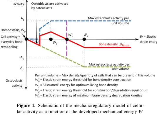
We want to keep a simplified approach in order to be able to identify the model’s parameters and to validate it. Our main assumption is that the cell activity is directly proportional to the intensity of the mechanical load, but with a predefined scenario. We define such a cell activity as the quantity of bone formation/resorption (or bone mineral density change) as a function of time and mechanical energy. Hence, for a given mechanical energy level, the cell activity will change the bone mineral density in a given time. The cell activity increases with the mechanical load up to a certain value that is proportional to the amount of available space within the structure (related to the porosity and defined in Figure 1by the maximum osteoblast activity per unit volume). The cell activity cannot exceed this value and a maximum cellular density exists. The maximum cellular activity (of osteoblasts or osteoclasts) is dependent on the cell density at a given location and at a given time. It is assumed that this activity linearly increases (with the mechanical load)
Figure 1. Schematic of the mechanoregulatory model of cellu-lar activity as a function of the developed mechanical energy W within the structure. Blue dashed line: osteoblast activity Aob. Green dashed line: osteoclast activity Aoc. Red line: bone density ρboneobtained by the combined blue and green cellular activities.
up to the maximum value (defined by the porosity). Finally, as we are working at the continuous macroscopic scale, we define a continuous representative volume element (RVE) that is large enough so that both osteoblasts and osteoclasts can be active within it at the same time (as a function of the given bone microstructure distribution and the given mechanical strain field) depending on the signals trans-mitted by the osteocytes. It is therefore assumed that the total bone mineral density change is the sum of the positive (through osteoblasts) and the negative (through osteoclasts) effects within this given RVE. Therefore, bone mineral density is di-rectly proportional to the cell activity and defined by the corresponding units (i.e., the cellular activity is given in kg · m−3·unit time−1 of fabricated (or degraded) bone per cell density).
A schematic of the cell activities as a function of the intensity of the developed mechanical energy W within the structure is presented inFigure 1. The homeosta-sis condition(W0) corresponds to the equilibrium state where it is acknowledged that bone remodeling and cellular activity are nonzero, but they are not integrated within the model. The modeled variations (i.e., bone density change) are dependent on cell activity differences away from the equilibrium state.
The osteoblast activity is shown as positive whereas the osteoclast activity is shown as negative. Both activities increase linearly up to a maximum level as the mechanical energy increases. Two conditions are required here:
(1) for a bone density increase for “medium low” mechanical energy(W0< W < W2), the osteoblast activity must be higher than the osteoclast one, and (2) for a bone density decrease with “higher” mechanical energy(W > W2), the
osteoclast activity must be higher than the osteoblast one.
On the graph inFigure 1, the initial osteoblast activity is triggered by osteoclasts (osteoblasts will start being active only after osteoclasts have “cleaned up” the bone surface so bone remodeling can initiate). At W0, we are at homeostasis state where neither bone formation nor resorption occurs at a constant living load condition. Only continuous bone remodeling of living is present. This means thatFigure 1is correct at a given time t and corresponds to an equilibrium state once bone forma-tion or degradaforma-tion has finished. In the current work, this condiforma-tion corresponds to the start of the analysis (initial zero condition). From W0 to W1, both osteoblast and osteoclast activity increase at the same time leading to an increase of the bone mineral density since the sum of both cell activities is positive. When reaching the maximum osteoblast activity, i.e., W ≥ W1, the bone mineral density increase is impacted by the osteoclast activity taking over the osteoblast one. Above a given energy threshold, from W2 to W3, the bone mineral density decreases as the combined cell effect is negative. For a mechanical energy between W0and W2, we have a bone density increase, while for a mechanical energy above W2, we have a bone density decrease. W2corresponds to the energy threshold not to overtake to keep a good bone health. The following equations interpret the scheme inFigure 1:
if W0< W < W1, then Aob=k1·W +ρboneini and Aoc= −k2·W +ρboneini , if W1< W < W2, then Aob=A1+ρboneini and Aoc= −k2·W +ρboneini , if W2< W < W3, then Aob=A1+ρboneini and Aoc= −k2·W +ρbone,ini if W> W3, then Aob=A1+ρboneini and Aoc= −A2+ρboneini ,
(1)
where k1and k2are the coefficients of osteoblast and osteoclast activity increase, A1and A2are their corresponding maximum values, andρboneini is the initial bone density, constant over time, in kg · m−3·unit time−1. Thus, we obtain a model with only four parameters (k1, k2, A1, and A2) defined as
Aob=k1·W +ρboneini for W< W1, Aoc= −k2·W +ρboneini for W< W3, Amaxob =A1+ρboneini for W> W1, Amaxoc = −A2+ρboneini for W> W3.
(2) The units of these four parameters are given in kg · m−3·unit time−1for A1and A2, and in kg · mJ−1·m−3·unit time−1for k1and k2. Such parameters can be quantified
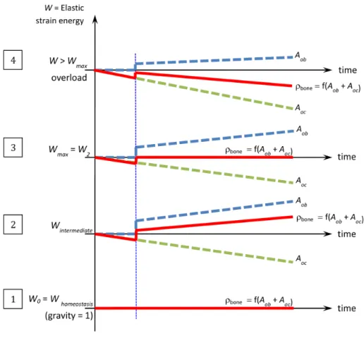
Figure 2. Schematic of the mechanoregulatory model or cellular activity as a function of time t for different levels of applied me-chanical load (energy) within the structure. Blue dashed line: os-teoblast activity Aob. Green dashed line: osteoclasts activity Aoc. Red line: bone densityρbone.
experimentally by histochemistry through the measurement of the different cell density activities as a function of the applied mechanical load at any given time and point of the structure. For instance, osteocyte viability and osteoclast activity can be determined through the ratio between empty (i.e., without cell) and full (i.e., with cell) lacunae. More specifically, osteocyte viability can be determined by cell apoptosis through cleaved caspase-3 activation[Lavrik 2005;Nicholson et al. 1995;Maurel et al. 2013], and osteoclast activity through the measure of the resorption area surrounding the cells (TRAP activity)[Kodama et al. 2009].
Once the cell activity has been defined and quantified as a function of the me-chanical energy W , we can describe it as a function of time for different levels of mechanical loads (as presented inFigure 2).
Four different cases are considered:
(1) When forces correspond to everyday life conditions, we are at equilibrium state(Whomeostasis) where the bone density is in the homeostasis condition. In this case, the “average” osteoblastic and osteoclastic cell activities are equal and opposite. Their sum is equal to zero (corresponding to homeostatic state) and bone mineral density remains constant over time.
(2) When forces increase(Wintermediate), corresponding to a “sport training”-like activity at a moderate level, osteoblastic cells become predominant and the sum of these effects is positive leading to an increase in the bone mineral density.
(3) If the “exercise” level increases (over-training-like) leading to an increase of the averaged developed mechanical energy, the energy level reaches a thresh-old(Wmax=W2) corresponding to the maximum energy under which bone density evolution remains at best positive or null. Here again, and similarly to the homeostasis case, but not for the same reason, the combined effect of osteoblasts and osteoclasts provides equilibrium. However, contrary to the homeostasis case, this equilibrium is unstable, depending on the biology that is patient-dependent.
(4) Finally, when the average mechanical energy goes beyond the threshold(W = W2), bone density decreases due to an over-expression of the osteoclastic cells reacting to a solicitation that needs to be biologically quantified.
In essence, an average person’s life is the result of the combined effect of all these different cases (being dependent on both the mechanical energy level and time) and bone mineral density evolves accordingly in space and time.
An interpretation of the schematic bone mineral density evolution in time of Figure 2is given by the four energy intervals
if W0< W < W1, then ∂ρbone ∂t > 0 and ρbone> 0, if W1< W < W2, then ∂ρbone ∂t < 0 and ρbone> 0, if W2< W < W3, then ∂ρbone ∂t < 0 and ρbone< 0, if W> W3, then ∂ρbone ∂t < 0 and ρbone< 0, (3)
whereρboneis the bone density.
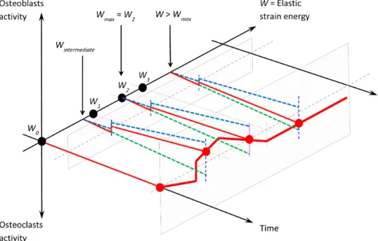
When combining the two schemes of Figures1and2on the same graph, we obtain the correspondingFigure 3where the bone mineral density is a function
Figure 3. Global schematic of the mechanoregulatory model or cell activity as a function of time and energy. Blue dashed line: osteoblast activity Aob. Green dashed line: osteoclast activity Aoc. Red line: bone densityρbone.
of time t and the elastic strain energy W (when we suppose that the mechanical behavior of bone is linear elastic).
As the cell activity is defined as an amount of fabricated (or degraded) bone as a function of its density, the amount of mechanical energy developed, and the time, the variation of bone mineral density can be computed directly. It remains only to calculate the corresponding Young’s modulus (as a function of the bone density), given by the relation E = E0·ρ2
bone [Rho et al. 1995], that is classically accepted in the literature, where E0is the cortical bone Young’s modulus.
2.2. Model application. A numerical application of the above proposed model is made on a simplified geometry accounting for simple load conditions. We consider a femur diaphysis loaded under compression (i.e., body weight) as presented in Figure 4, left. Since we assume a constant distribution of the stresses through the thickness of the femur diaphysis, we propose to study a simplified 2D rectangular beam of length L = 50 mm and height H = 20 mm (Figure 4, right).
Of course, it is acknowledged that the exact quantification of the model param-eters will depend on the given geometry and structure of the exact experimental model to represent. In this case, we will quantify them only for validation purposes.
Figure 4. Geometry for the numerical application. Left: real ge-ometry of a femoral diaphysis under simple tension. Right: sim-plified geometry of a rectangular beam under simple tension.
The other material parameters are defined by the Young’s modulus of the cortical bone E0=20.3 GPa and Poisson ratio ν = 0.3[Bernard et al. 2013]. The applied mechanical load is equivalent to a human body weight F = 400 N on one leg and an initial normalized bone densityρboneini =0.5 is taken for validation purposes. We suppose a closed system with no external input.
The model parameters were identified without a priori knowledge of the corre-sponding biological quantifications of the in vivo conditions and serve here only for validation. The homeostatic energy W0=1 × 10⁻⁵mJ was determined based on an average femur cross-sectional area and its corresponding bone density and body weight load conditions. The other two energies W1=1.456 × 10⁻⁵mJ and W3=3 × 10⁻⁵mJ were defined based on identification of the four parameters of the model by k1=1×10⁵kg·mJ−1·m−3·unit time−1, k2=0.7×10⁵kg·mJ−1·m−3· unit time−1, A1=1.456 kg·m−3·unit time−1, and A2=2 kg·mJ−1·m−3·unit time−1, where k1> k2and A2> A1. The intermediate energy W2is the linear interpolation between W1and W3. The model was implemented within the software COMSOL Multiphysics, and the results are presented in the following section.
3. Results and discussion
3.1. Validation. The model was subjected to a constant force F = 400 N, corre-sponding to the body weight, for an arbitrary length of time, leading to a constant energy distribution throughout the structure and hence a bone density evolution as defined byFigure 3. An initial numerical validation of the model was made by testing three simplified cases: (i) osteoblasts and osteoclasts have the same activity (i.e., the models parameters are equal and opposite: k1= −k2 and A1= −A2), (ii) only osteoblasts are active (i.e., k2 = A2=0), and (iii) only osteoclasts are active (i.e., k1=A1=0). The results are presented inFigure 5.
As expected, an equal intensity of osteoblast and osteoclast activity (Figure 5, left) leads to a constant bone density as a function of time. This is similar to home-ostasis conditions when homogenized to long periods of time (everyday life activ-ity). InFigure 5, center, when only osteoblasts are considered (i.e., k2=A2=0), there is no osteoclast activity; therefore, if the energy level is high enough to trigger
Figure 5. Evolution of the model parameters, bone density, and mechanical energy as a function of time for the three simplified cases.
Figure 6. Mechanical energy W variation as function of time for different values of the applied force F .
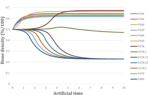
osteoblasts, bone density increases and since the bone stiffness increases corre-spondingly, then the developed mechanical energy (for a constant applied force) decreases, and so does the osteoblast activity. Finally, when only osteoclasts are considered (i.e., k1=A1=0, inFigure 5, right), there is no osteoblast activity, bone density decreases and so does its stiffness, and hence the developed mechanical energy increases (for a constant applied force) together with the osteoclast activity. 3.2. Results and sensitivity study for different load cases. Different intensities of F were applied from 360 N to 480 N. The results are presented in Figures6, 7, and8. For constant-load cases below 478 N, we observe a convergence towards an increase of bone density (Figure 7) and a corresponding decrease of mechanical energy (Figure 6). For load cases above 478 N, the opposite occurs with a decrease
Figure 7. Bone mineral densityρbonevariation as function of time for different values of the applied force F .
of bone density and an increase of energy. Here, the energy threshold W2 shows up around 478.1 N with the given values of the model parameters.
The threshold (i.e., the switch from positive to negative bone density) is very sensitive to the intensity of the applied force and it is located within a very thin force range around 478 N, deregulating the system very quickly. It is not possible at this stage to know if this is a limitation of the proposed model (due to the simplified as-sumptions made or the lack of more detailed information on the existing couplings at the mechanobiological level) or if this is really occurring in reality. Such an aspect needs to be investigated further experimentally at a later stage. For the case of the control force (400 N), the mechanical energy W and the bone densityρbone reach final values of 9.019 × 10⁻⁶mJ and 0.64.
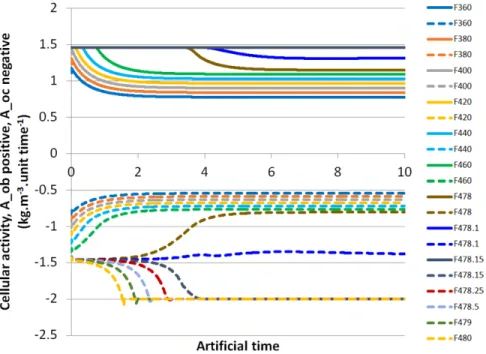
Cell activities are presented inFigure 8. For the control case, their final values are equal to 9.019 × 10⁻¹kg · m−3·unit time−1 and −6.313 × 10⁻¹kg · m−3· unit time−1 for Aob and Aoc, respectively. Thus, we can conclude that for this specific case, a fast stabilization is observed to reach the mechanobiological equi-librium. Since we observed a fast switch in the variable trends around 478 N, we decided to perform more simulations around this threshold in order to highlight such a transition.
Similarly to the developed mechanical energy and bone mineral density varia-tions, when the applied mechanical force increases above 478 N, osteoblast activity reaches its maximum value, and we observe an inversion of the osteoclast activity
Figure 8. Osteoblast activity Aoband osteoclast activity Aoc vari-ations as functions of time for different values of the applied force F . Osteoblast activity is shown positive in continuous lines up to a force of 478.15 N above which it remains maximal at 1.46 kg · m−3·unit time−1. Osteoclast activity is shown negative in dashed lines up to a force of 480 N showing the transient behavior through 478 N towards bone degradation.
(decreasing to increasing). As the osteoblast activity is at its maximum of 1.46 kg · m−3·unit time−1, when increasing the applied force, the osteoclast activity will pass from “ineffective” (below the osteoblast activity of −1.5 kg·m−3·unit-time−1) to “effective” as it reaches a final value of −2 kg · m−3·unit time−1. Once the new equilibrium reached, where both osteoblast and osteoclast activities have reached their maximum value, a fast bone degradation is observed (Figure 7). A return to normal physical conditions depends upon a decrease of the applied mechanical force and a new stabilization of the system under study.
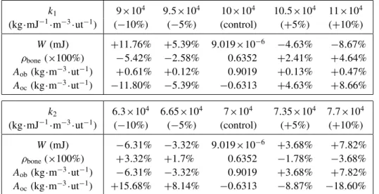
The proposed model only relies on a few parameters: ρboneini , A1, A2, k1, k2, W0, W1, and W3. A sensitivity study was performed in order to evaluate their influence on the overall results. We vary one parameter at a time in the range ±10% and we recorded the obtained results for the energy W , the osteoblast ( Aob) and osteoclast ( Aoc) activities, and the bone densityρbone. The obtained results show thatρboneini , A1, A2, W0, W1, and W3, within the 10% range variation, have
k1 9×10⁴ 9.5×10⁴ 10×104 10.5×10⁴ 11×104 (kg·mJ−1·m−3·ut−1) (−10%) (−5%) (control) (+5%) (+10%) W (mJ) +11.76% +5.39% 9.019×10⁻⁶ −4.63% −8.67% ρbone(×100%) −5.42% −2.58% 0.6352 +2.41% +4.64% Aob(kg·m−3·ut−1) +0.61% +0.12% 0.9019 +0.13% +0.47% Aoc(kg·m−3·ut−1) −11.80% −5.39% −0.6313 +4.63% +8.66% k2 6.3×10⁴ 6.65×10⁴ 7×10⁴ 7.35×10⁴ 7.7×10⁴ (kg·mJ−1·m−3·ut−1) (−10%) (−5%) (control) (+5%) (+10%) W (mJ) −6.31% −3.32% 9.019×10⁻⁶ +3.68% +7.82% ρbone(×100%) +3.32% +1.7% 0.6352 −1.78% −3.68% Aob(kg·m−3·ut−1) −6.31% −3.32% 0.9019 +3.68% +7.82% Aoc(kg·m−3·ut−1) +15.68% +8.14% −0.6313 −8.87% −18.60%
Table 1. Results of the sensitivity study performed for k1 and k2, where “ut” stands for “unit time”.
little effect. The initial bone mineral density value has no effect since we apply a constant force on the structure, so whatever the initial state equilibrium, it will lead to the same final results with a different kinematic evolution. Since most of the evolution occurs during the osteoblast ( Aob) and osteoclast ( Aoc) activities through k1and k2 parameters, the other parameters do not impact either of the obtained results in this study.
However, it appeared that k1 and k2 have a higher impact on the final results as reported inTable 1. As k1decreases,ρbone decreases too(−11.8%), whereas as k2decreases,ρbone increases(+15.68%). For W and Aob, inverse trends can be noticed when varying k1and k2. For k1, W and Aobfluctuate between +11.76% and −8.67% and between −5.42% and +4.64%, respectively. For k2, W and Aobfluctuate between −6.31% and +7.82% and between +3.32% and −3.68%, respectively. Finally, Aocvaries between +0.61% and +0.47% for k1 and between +6.31% and +7.82% for k2.
Most of the bone mineral density variation occurs within the k1and k2phases. Hence, modifying only one parameter (k1or k2) at a time has a direct impact on the final results. This effect would be compensated for if both parameters would change oppositely in the same proportions, which would lead to the same final results.
After identification and validation of the mechanobiological phenomena at play in this model (developed mechanical energy, osteoblast and osteoclast activities, and bone mineral density variations) as a function of time for given intensities of mechanical forces, the results were plotted not as a function of time, but as a
Figure 9. Numerical results (in comparison to the initial model hypotheses ofFigure 1).
function of the intensity of mechanical energy for all the simulations. The results are presented inFigure 9.
Figure 9shows the results obtained with the newly proposed mechanoregulatory model. These results should be compared withFigure 1showing the theoretical hypotheses defined initially. An observation is made that a very strong correlation is obtained between the proposed model and the obtained numerical results. We have an initial increase of the osteoblast and osteoclast activities up to their max-imum values that remain constant afterwards. The only difference is that in the numerical model, the initial osteoblast activity being triggered by the osteoclasts was not included, which explains why it is not visible inFigure 9, but starts directly increasing at the origin. We also observe that the bone mineral density evolution follows the sum of both cell activities (function of the applied mechanical force) being positive initially for lower mechanical energy and negative later on for higher energy from an original normalized bone density of 0.5. The maximum osteoblast activity is reached first (energy level W1) followed by the maximum of the osteo-clast activity (energy level W3). We note that the equilibrium between osteoblast and osteoclast activity does not correspond to the bone mineral density variation equaling zero (i.e., a return to the initial bone density of 0.5) as there appears to be a time delay of the structure response to the mechanical load. The passage of the bone mineral density from positive to negative variation occurs later. Thereafter, there is a continuing decrease of the bone mineral density with stabilization later on, dependent on the intensity of the applied force.
3.3. Application to variable load conditions. The numerical results were validated on constant load and showed good correlation with the proposed model hypotheses.
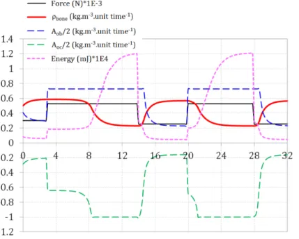
Figure 10. Bone mineral density, cell activity, and energy varia-tions when applying a variable force below and above the degra-dation threshold (overload threshold).
Hence, to extract bone density variations in a more “real application”-like environ-ment, variable mechanical forces were considered. A constant force is applied on the model until equilibrium is reached (constant bone density that occurs in normal living conditions after several weeks). Then the intensity of the applied force is changed to reach a new equilibrium. This is done for two intensities of the mechanical force, one below and one above the overload degradation threshold. Results are presented inFigure 10.
At initial mechanical load (300 N), bone density quickly reaches equilibrium (≈ 0.55) with decreasing cellular activity. Next, the force is increased above the threshold (520 N). The cell activity is changed to reach its maximum with imme-diate response from osteoblasts and delayed response from osteoclasts. This is dependent on the evolution of the elastic strain energy within the model that takes time to develop as a function of the bone density that is present at a given point of the structure and at a given time. Once the energy has developed above the thresh-old, bone density starts to decrease to reach a new equilibrium that is lower than the previous one. When cycling this effect by applying in turn these two mechanical forces, we observe the corresponding bone density variations and new equilibrium being formed. Decreasing the overloading force will lead to a reincrease of the
bone density coming back to its “normal” healthy working conditions. However, it is anticipated that keeping an overload condition on the bone will probably lead to a complete degradation of the structure. This was not modeled here as it certainly requires accounting for extra mechanobiological actions that were not integrated within this simplified mechanoregulatory model.
4. Conclusion
A new comprehensive approach based on cell activity to describe bone remod-eling is proposed to assess the possible bone degradation kinetics when under high-intensity mechanical loads. Despite the complexity of the mechanobiological process, only four experimentally measurable parameters are required to tune this model for specific cases. These are the variations of the bone density kinetics with the intensity of the applied mechanical loads up to their maximum value, and the two maximum values for osteoblasts and osteoclasts activities. The results show the respective contributions of each process on the bone mineral density evolution and are in agreement with the experimental data provided in the literature. In fact, the model is able to depict both the harmful and the favorable effects of high and medium mechanical loads, respectively. With this approach, when experimentally measuring the four model parameters for different load scenario (force intensity, test specimen, aging, diseased, etc.), potential differences are expected between the cases and possible foreseen applications for the optimization process for sport activities.
Acknowledgements
The authors would like to thank the CNRS for its financial support through the Défi Mécanobiologie to carry out the work.
References
[Allena and Maini 2014] R. Allena and P. K. Maini, “Reaction–diffusion finite element model of lateral line primordium migration to explore cell leadership”, B. Math. Bio. 76:12 (2014), 3028– 3050.
[Andreaus et al. 2014a] U. Andreaus, M. Colloca, and D. Iacoviello,“Optimal bone density distri-butions: numerical analysis of the osteocyte spatial influence in bone remodeling”, Comput. Meth. Prog. Bio.113:1 (2014), 80–91.
[Andreaus et al. 2014b] U. Andreaus, I. Giorgio, and T. Lekszycki,“A 2-D continuum model of a mixture of bone tissue and bio-resorbable material for simulating mass density redistribution under load slowly variable in time”, Z. Angew. Math. Mech. 94:12 (2014), 978–1000.
[Bagherian et al. 2019] A. Bagherian, M. Baghani, D. George, Y. Rémond, C. Chappard, S. Pat-lazhan, and M. Baniassadi,“A novel numerical model for the prediction of patient-dependent bone density loss in microgravity based on micro-CT images”, Continuum Mech. Therm. 32:3 (2019), 927–943.
[Beaupré et al. 1990] G. S. Beaupré, T. E. Orr, and D. R. Carter,“An approach for time-dependent bone modeling and remodeling-application: a preliminary remodeling simulation”, J. Orthop. Res. 8:5 (1990), 662–670.
[Bednarczyk and Lekszycki 2016] E. Bednarczyk and T. Lekszycki,“A novel mathematical model for growth of capillaries and nutrient supply with application to prediction of osteophyte onset”, Z. Angew. Math. Phys.67:4 (2016), art. id. 94.
[Bernard et al. 2013] S. Bernard, Q. Grimal, and P. Laugier,“Accurate measurement of cortical bone elasticity tensor with resonant ultrasound spectroscopy”, J. Mech. Behav. Biomed. 18 (2013), 12–19.
[Burr and Allen 2014] D. B. Burr and M. R. Allen,“Bone modeling and remodeling”, Chapter 4, pp. 75–90 in Basic and applied bone biology, edited by D. B. Burr and M. R. Allen, Academic, London, 2014.
[Carter 1984] D. R. Carter,“Mechanical loading histories and cortical bone remodeling”, Calcified Tissue Int.36:S1 (1984), S19–S24.
[Cowin 1986] S. C. Cowin,“Wolff’s law of trabecular architecture at remodeling equilibrium”, J. Biomech. Eng.108:1 (1986), 83–88.
[Ehrlich and Lanyon 2002] P. J. Ehrlich and L. E. Lanyon,“Mechanical strain and bone cell function: a review”, Osteoporosis Int. 13:9 (2002), 688–700.
[Forwood and Parker 1989] M. R. Forwood and A. W. Parker,“Microdamage in response to repeti-tive torsional loading in the rat tibia”, Calcified Tissue Int. 45:1 (1989), 47–53.
[Frame et al. 2018] J. Frame, P.-Y. Rohan, L. Corté, and R. Allena,“Optimal bone structure is dependent on the interplay between mechanics and cellular activities”, Mech. Res. Commun. 92 (2018), 43–48.
[Frame et al. 2019] J. Frame, P.-Y. Rohan, L. Corté, and R. Allena,“A mechano-biological model of multi-tissue evolution in bone”, Continuum Mech. Therm. 31:1 (2019), 1–31.
[Frost 1987] H. M. Frost,“Bone ‘mass’ and the ‘mechanostat’: a proposal”, Anat. Rec. 219:1 (1987), 1–9.
[George et al. 2017] D. George, C. Spingarn, C. Dissaux, M. Nierenberger, R. A. Rahman, and Y. Rémond,“Examples of multiscale and multiphysics numerical modeling of biological tissues”, Bio-Med. Mater. Eng.28:S1 (2017), S15–S27.
[George et al. 2018a] D. George, R. Allena, and Y. Rémond,“Cell nutriments and motility for mechanobiological bone remodeling in the context of orthodontic periodontal ligament deforma-tion”, J. Cell. Immunoth. 4:1 (2018), 26–29.
[George et al. 2018b] D. George, R. Allena, and Y. Rémond,“A multiphysics stimulus for continuum mechanics bone remodeling”, Math. Mech. Complex Syst. 6:4 (2018), 307–319.
[George et al. 2019] D. George, R. Allena, and Y. Rémond,“Integrating molecular and cellular kinetics into a coupled continuum mechanobiological stimulus for bone reconstruction”, Continuum Mech. Therm.31:3 (2019), 725–740.
[Giorgio et al. 2016] I. Giorgio, U. Andreaus, D. Scerrato, and F. dell’Isola,“A visco-poroelastic model of functional adaptation in bones reconstructed with bio-resorbable materials”, Biomech. Model. Mechan.15:5 (2016), 1325–1343.
[Giorgio et al. 2017] I. Giorgio, U. Andreaus, F. dell’Isola, and T. Lekszycki,“Viscous second gradient porous materials for bones reconstructed with bio-resorbable grafts”, Extreme Mech. Let. 13 (2017), 141–147.
[Grimston et al. 1991] S. K. Grimston, J. R. Engsberg, R. Kloiber, and D. A. Hanley,“Bone mass, external loads, and stress fracture in female runners”, Int. J. Sport Biomech. 7:3 (1991), 293–302.
[Hao et al. 2017] L. Hao, L. Rui-Xin, H. Biao, Z. Bin, H. Bao-Hui, L. Ying-Jie, and Z. Xi-Zheng,
“Effect of athletic fatigue damage and the associated bone targeted remodeling in the rat ulna”, Biomed. Eng. Online 16:1 (2017).
[Herman et al. 2010] B. C. Herman, L. Cardoso, R. J. Majeska, K. J. Jepsen, and M. B. Schaffler,
“Activation of bone remodeling after fatigue: differential response to linear microcracks and diffuse damage”, Bone 47:4 (2010), 766–772.
[Ignatius et al. 2005] A. Ignatius, H. Blessing, A. Liedert, C. Schmidt, C. Neidlinger-Wilke, D. Kaspar, B. Friemert, and L. Claes,“Tissue engineering of bone: effects of mechanical strain on osteoblastic cells in type I collagen matrices”, Biomaterials 26:3 (2005), 311–318.
[Klein-Nulend et al. 2013] J. Klein-Nulend, A. D. Bakker, R. G. Bacabac, A. Vatsa, and S. Wein-baum,“Mechanosensation and transduction in osteocytes”, Bone 54:2 (2013), 182–190.
[Kodama et al. 2009] H. Kodama, A. Yamasaki, M. Abe, S. Niida, Y. Hakeda, and H. Kawashima,
“Transient recruitment of osteoclasts and expression of their function in osteopetrotic (op/op) mice by a single injection of macrophage colony-stimulating factor”, J. Bone Miner. Res. 8:1 (2009), 45–50.
[Lavrik 2005] I. N. Lavrik,“Caspases: pharmacological manipulation of cell death”, J. Clin. Invest. 115:10 (2005), 2665–2672.
[Lekszycki 2002] T. Lekszycki,“Modelling of bone adaptation based on an optimal response hy-pothesis”, Meccanica 37:4–5 (2002), 343–354.
[Lekszycki and dell’Isola 2012] T. Lekszycki and F. dell’Isola,“A mixture model with evolving mass densities for describing synthesis and resorption phenomena in bones reconstructed with bio-resorbable materials”, Z. Angew. Math. Mech. 92:6 (2012), 426–444.
[Lemaire et al. 2005] T. Lemaire, S. Naïli, and A. Rémond,“Multiscale analysis of the coupled effects governing the movement of interstitial fluid in cortical bone”, Biomech. Model. Mechan. 5:1 (2005), 39–52.
[Lemaire et al. 2010] T. Lemaire, S. Naili, and V. Sansalone,“Multiphysical modelling of fluid transport through osteo-articular media”, An. Acad. Bras. Ciênc. 82:1 (2010), 127–144.
[Lemaire et al. 2011] T. Lemaire, E. Capiez-Lernout, J. Kaiser, S. Naili, and V. Sansalone,“What is the importance of multiphysical phenomena in bone remodelling signals expression? A multiscale perspective”, J. Mech. Behav. Biomed. 4:6 (2011), 909–920.
[Lemaire et al. 2015] T. Lemaire, J. Kaiser, S. Naili, and V. Sansalone,“Three-scale multiphysics modeling of transport phenomena within cortical bone”, Math. Probl. Eng. (2015), art. id. 398970. [Louna et al. 2016] Z. Louna, I. Goda, J.-F. Ganghoffer, and S. Benhadid,“Formulation of an
effec-tive growth response of trabecular bone based on micromechanical analyses at the trabecular level”, Arch. Appl. Mech.87:3 (2016), 457–477.
[Lu and Lekszycki 2016] Y. Lu and T. Lekszycki,“A novel coupled system of non-local integro-differential equations modelling Young’s modulus evolution, nutrients’ supply and consumption during bone fracture healing”, Z. Angew. Math. Phys. 67:5 (2016), art. id. 111.
[Madeo et al. 2011] A. Madeo, T. Lekszycki, and F. dell’Isola,“A continuum model for the bio-mechanical interactions between living tissue and bio-resorbable graft after bone reconstructive surgery”, C. R. Mécanique 339:10 (2011), 625–640.
[Madeo et al. 2012] A. Madeo, D. George, T. Lekszycki, M. Nierenberger, and Y. Rémond,“A second gradient continuum model accounting for some effects of micro-structure on reconstructed bone remodelling”, C. R. Mécanique 340:8 (2012), 575–589.
[Martin et al. 2017] M. Martin, T. Lemaire, G. Haïat, P. Pivonka, and V. Sansalone,“A thermody-namically consistent model of bone rotary remodeling: a 2D study”, Comput. Method. Biomech. Biomed.20:S1 (2017), S127–S128.
[Maurel et al. 2013] D. B. Maurel, D. Benaitreau, C. Jaffré, H. Toumi, H. Portier, R. Uzbekov, C. Pichon, C. L. Benhamou, E. Lespessailles, and S. Pallu,“Effect of the alcohol consumption on osteocyte cell processes: a molecular imaging study”, J. Cell. Mol. Med. 18:8 (2013), 1680–1693. [Nicholson et al. 1995] D. W. Nicholson, A. Ali, N. A. Thornberry, J. P. Vaillancourt, C. K. Ding,
M. Gallant, Y. Gareau, P. R. Griffin, M. Labelle, Y. A. Lazebnik, N. A. Munday, S. M. Raju, M. E. Smulson, T.-T. Yamin, V. L. Yu, and D. K. Miller,“Identification and inhibition of the ICE/CED-3 protease necessary for mammalian apoptosis”, Nature 376:6535 (1995), 37–43.
[Pivonka and Komarova 2010] P. Pivonka and S. V. Komarova,“Mathematical modeling in bone biology: From intracellular signaling to tissue mechanics”, Bone 47:2 (2010), 181–189.
[Pivonka et al. 2008] P. Pivonka, J. Zimak, D. W. Smith, B. S. Gardiner, C. R. Dunstan, N. A. Sims, T. J. Martin, and G. R. Mundy,“Model structure and control of bone remodeling: a theoretical study”, Bone 43:2 (2008), 249–263.
[Rémond et al. 2016] Y. Rémond, S. Ahzi, M. Baniassadi, and H. Garmestani,Applied RVE recon-struction and homogenization of heterogeneous materials, Wiley, Hoboken, NJ, 2016.
[Rho et al. 1995] J. Y. Rho, M. C. Hobatho, and R. B. Ashman,“Relations of mechanical properties to density and CT numbers in human bone”, Med. Eng. Phys. 17:5 (1995), 347–355.
[Rochefort et al. 2010] G. Y. Rochefort, S. Pallu, and C. L. Benhamou,“Osteocyte: the unrecognized side of bone tissue”, Osteoporosis Int. 21:9 (2010), 1457–1469.
[Ruimerman et al. 2005] R. Ruimerman, P. Hilbers, B. van Rietbergen, and R. Huiskes,“A theo-retical framework for strain-related trabecular bone maintenance and adaptation”, J. Biomech. 38:4 (2005), 931–941.
[Sansalone et al. 2015] V. Sansalone, D. Gagliardi, C. Desceliers, G. Haïat, and S. Naili,“On the un-certainty propagation in multiscale modeling of cortical bone elasticity”, Comput. Method. Biomech. Biomed.18:S1 (2015), 2054–2055.
[Scala et al. 2017] I. Scala, C. Spingarn, Y. Rémond, A. Madeo, and D. George, “Mechanically-driven bone remodeling simulation: application to LIPUS treated rat calvarial defects”, Math. Mech. Solids22:10 (2017), 1976–1988.
[Schmitt et al. 2015] M. Schmitt, R. Allena, T. Schouman, S. Frasca, J. M. Collombet, X. Holy, and P. Rouch,“Diffusion model to describe osteogenesis within a porous titanium scaffold”, Comput. Method. Biomech. Biomed.19:2 (2015), 171–179.
[Sheidaei et al. 2019] A. Sheidaei, M. Kazempour, A. Hasanabadi, F. Nosouhi, M. Pithioux, M. Baniassadi, Y. Rémond, and D. George,“Influence of bone microstructure distribution on developed mechanical energy for bone remodeling using a statistical reconstruction method”, Math. Mech. Solids24:10 (2019), 3027–3041.
[Spingarn et al. 2017] C. Spingarn, D. Wagner, Y. Rémond, and D. George,“Multiphysics of bone remodeling: a 2D mesoscale activation simulation”, Bio-Med. Mater. Eng. 28:S1 (2017), S153– S158.
[Turner 1998] C. H. Turner, “Three rules for bone adaptation to mechanical stimuli”, Bone 23:5 (1998), 399–407.
DANIELGEORGE: george@unistra.fr
ICube Laboratory, Université de Strasbourg, Centre National de la Recherche Scientifique, Strasbourg, France
RACHELEALLENA: rachele.allena@ensam.eu
Institut de Biomécanique Humaine Georges Charpak, Arts et Métiers ParisTech, Paris, France CÉLINEBOURZAC: celine.bourzac@vet-alfort.fr
Institut National de la Santé et de la Recherche Médicale, Université Paris Sciences et Lettres, Centre National de la Recherche Scientifique, Paris, France
STÉPHANEPALLU: stephane.pallu@univ-orleans.fr
Institut National de la Santé et de la Recherche Médicale, Université Paris Sciences et Lettres, Centre National de la Recherche Scientifique, Paris, France
and Collégium Sciences et Techniques, Université d’Orléans, Orléans, France MORAD BENSIDHOUM: morad.bensidhoum@paris7.jussieu.fr
Institut National de la Santé et de la Recherche Médicale, Université Paris Sciences et Lettres, Centre National de la Recherche Scientifique, Paris, France
HUGUES PORTIER: hugues.portier@univ-orleans.fr
Institut National de la Santé et de la Recherche Médicale, Université Paris Sciences et Lettres, Centre National de la Recherche Scientifique, Paris, France
and Collégium Sciences et Techniques, Université d’Orléans, Orléans, France YVESRÉMOND: remond@unistra.fr
ICube Laboratory, Université de Strasbourg, Centre National de la Recherche Scientifique, Strasbourg, France