Technology researchers and makes it freely available over the web where possible.
This is an author-deposited version published in: https://sam.ensam.eu
Handle ID: .http://hdl.handle.net/10985/20056
To cite this version :
L. MONTIER, T. HENNERON, S. CLENET, B. GOURSAUD - Model Order Reduction applied to a linear Finite Element model of a squirrel cage induction machine based on POD approach - IEEE Transactions on Magnetics p.1-4 - 2021
Any correspondence concerning this service should be sent to the repository Administrator : [email protected]
Model Order Reduction applied to a linear Finite Element model of
a squirrel cage induction machine based on POD approach
L. Montier
1,2, T. Henneron
1S. Cl´enet
1and B. Goursaud
21Univ. Lille, Centrale Lille, Arts et Metiers ParisTech, HEI, EA 2697 - L2EP, F-59000 Lille, France 2EDF R&D, ERMES, 7 Boulevard Gaspard Monge, 91120 Palaiseau, France
The Proper Orthogonal Decomposition (POD) approach is applied to a linear Finite Element (FE) model of a squirrel cage induction machine. In order to obtain a reduced model valid on the whole operating range, snapshots are extracted from the simulation of typical tests such as at locked rotor and at the synchronous speed. Then, the reduced model of the induction machine is used to simulate different operating points with variable rotation speed and the results are compared to the full FE model to show the effectiveness of the proposed approach.
Index Terms—Induction machine, Magneto-quasistatic, Proper Orthogonal decomposition.
I. INTRODUCTION
T
O study low frequency electromagnetic devices, the FE method is commonly used. This approach gives accurate results but requires large computational times when the size of mesh and the number of time steps are important. In this context, this is difficult to use a FE model for the cosimulation of an electrical machine over a given operating cycle taking into account its electrical or/and mechanical environment. Then, Model Order Reduction (MOR) methods have been proposed in the literature to reduce the size of numerical models. The most popular approach is the Proper Orthogonal Decomposition (POD) [1]. Based on the solutions of the FE model (snapshots), a reduced basis is constructed where the solution of the reduced model is sought. This reduced basis should approximate correctly the solution for any operating point. In electrical engineering, it is well known that to characterize in practice the behavior of an electrical machine, typical tests (at no load, in short circuit...) are carried out. The idea is then to construct the reduced basis from snapshots extracted from the simulation of such tests. The approach has been applied to magnetostatic problems in order to determine reduced models of a three-phase transformer [2] for different loads and of a synchronous machine for different speeds [3]. In this article, we propose to apply this approach in the case of a linear magneto-quasistatic problem in order to define a reduced model of a squirrel cage induction machine valid its whole operating range [4]. To the author’s knowledge, MOR with POD of an induction machine accounting for the move-ment and for any speed slip has not been treated yet. First, the numerical model based on the FE method of the induction machine is presented. Secondly, the proposed approach to build a reduced model valid on the whole operating range is developed. In this case, the POD will be based on snapshots extracted from the simulation of typical tests such as at locked rotor and at the synchronous speed. Finally, the reduced model is used to study different operating points and the start-up of the machine for different load torques.Manuscript received December 1, 2012; revised August 26, 2015. Corre-sponding author: T. Henneron (email: [email protected]).
II. NUMERICALMODEL OF A SQUIRREL CAGE INDUCTION MACHINE
A. Continuous formulation
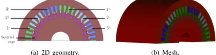
Let consider a squirrel cage induction machine presented on Fig. (1-a). The effect of the end ring is not taken into account in this study leading to a 2D extruded model. The mesh is composed of 10758 prism elements (Fig. (1-b)).
(a) 2D geometry. (b) Mesh. Fig. 1. Squirrel cage induction machine.
The mathematical formulation to be solved is based on a Magneto-Quasistatic problem. In this condition, we consider the Maxwell’s equations without displacement current,
curlH = Jind+ 3 X j=1 Njij (1) curlE = −∂B ∂t (2) divB = 0 (3)
divJind = 0 and divNj = 0 (4)
with B the magnetic flux density, H the magnetic field, E the electric field, Jind the eddy current density in the
conducting domain (i.e. the squirrel cage) and Nj and ij the
unit current density vector and the current flowing through the winding j. In the linear case, the magnetic behavior law is defined by B = µH = µ0µrH with µ0 the magnetic
permeability of the vacuum and µr the relative permeability.
In the squirrel cage, the electric behavior law is Jind = σE
with σ the electric conductivity. To impose the unicity of the solution, boundary conditions must be considered. To solve the problem, the A formulation can be used. A magnetic vector potential A is defined in the whole domain from (3) such as
B = curlA. From (2), the electric field can be expressed by E = −∂A∂t − U gradα with U the unknown representing the electric potential difference between the two extremities of the squirrel cage and α a given scalar function [5]. Then, based on (1) and (4-a), the strong formulation to be solved is
curlνcurlA + σ(∂A ∂t + U gradα) = 3 X j=1 Njij (5) divσ(∂A ∂t + U gradα) = 0 (6) with ν = 1/µ. The induction machine is supplied by a three-phase sinusoidal voltages system. To impose the voltage Vj at
the terminals of the winding j, the following relation is added, dΦj
dt + Rij = Vj with Φj = Z
Dj
A · Njdx (7)
with R the resistance of windings and Φj and Dj the linkage
magnetic flux and the subdomain associated with the winding j. In this condition, the currents ij with j = 1, 2, 3 are
also unknowns of the problem. In order to take into account variations of the rotation speed, the mechanical equation is introduced
JdΩ
dt + f Ω = Γem− Γr (8) with Ω the rotation speed, J the moment of rotor inertia, f the viscous coefficient, Γemthe electromagnetic torque depending
on B and Γr the load torque.
B. Discrete formulation
The fields A and Nj are discretised using edge and facet
elements and the scalar function α using the nodal elements. We denote by XA ∈ Rn the vector of Degrees of Freedom
(DoF) of A with n = 5507 the number of DoF. The numerical model of (5) and (6) is based on the Finite Element method. Then, the full numerical model is composed of a strong coupling between the FE model and the electric equations (7) and of a weak coupling with the mechanical equation (8). At each time step k, we solve the equation system
[MνXX+ M(θk−1) + MσXX∆t−1]XA,k+ CσXUUk − 3 X j=1 Fjij,k= MσXX∆t −1X A,k−1 (9) CσtXU∆t−1XA,k+ MσU UUk= CσtXU∆t−1XA,k−1 (10) Ftj∆t−1XA,k+ Rij,k= Vj,k+ Ftj∆t −1X A,k−1 (11) for j = 1, 2, 3.
Where ∆t is the time step, Ytis the transpose of the matrix Y, Fj is the vector depending on Nj and M(θk−1) is the
matrix deduced from the Overlapping method used to take into account the movement of the rotor [6]. The electromagnetic torque Γem,k is computed by Γem,k = XtA,kMvwXA,k with
Mvwthe matrix deduced from the Virtual Work method. Then,
the rotation speed Ωk is calculated with a weak coupling by
Ωk= (1 −
f ∆t
J )Ωk−1+ ∆t
J (Γem,k− Γr). (12)
III. MODELORDERREDUCTION BASED ONPODMETHOD
A. Structure of the reduced model
The idea is to build a reduced model of the equation system of the full model depending on XA in order to conserve the
structure of the system to be solved. Based on solutions, called snapshots, of the full model concatened into a matrix SX
such as SX = [XA,1; XA,2; ...; XA,N] with N the number of
snapshots, a reduced basis is constructed from the Singular Value Decomposition such as SX = USVt with Un×n
and VN ×N orthogonal matrices and Sn×N the matrix of
the singular values. The reduced basis Ψ is defined by the m first columns of U such as Ψ = [U1; U2; ...; Um]. The
truncation of the m first columns can be determined by taking the most significative singular values of S. The vector of DoF’s XAr of the reduced model is defined by XA = ΨXAr with
XAr∈ Rm. To construct the reduced model, XA,kis replaced
by ΨXAr,k in (9), (10) and (11). The equation system is
then overdetermined since the number of equations n is much higher than the number of unknowns m. To obtain a well posed equation system, equation (9) is projected into the reduced basis by multiplying by Ψt. Finally, at each time step k, the
reduced model to be solved is
[MνXXr+ Mr(θk−1) + MXXrσ ∆t−1]XAr,k+ CσXU rUk − 3 X j=1 Frjij,k= MσXXr∆t −1X Ar,k−1 (13) CσtXU r∆t−1XAr,k+ MσU UUk= CσtXU r∆t−1XAr,k−1 (14) Ftr1∆t−1XAr,k+ Rij,k= Vj,k+ Ftr1∆t −1X Ar,k−1 (15) for j = 1, 2, 3. with Mν rXX = ΨtMνXXΨ, Mr(θk−1) = ΨtM(θj−1)Ψ, MσXXr = ΨtMσXXΨ, CXU rσ = Ψ tCσ XU and Fjr = ΨtFj.
The torque Γem can be expressed in function of XAr,k by
Γem,k = XtAr,kMvwrXAr,k with Mvwr = ΨtMvwΨ. We
can note that the matrix Mr(θk−1) is recomputed at each time
step k. However, the computation cost is limited due to the size of this matrix which corresponds to unknowns on a subdomain located in the air gap of the machine.
B. Construction of the reduced basis valid on the whole operating range
In order to define a reduced model valid on the whole operating range of the induction machine, Nsync and Nlr
snapshots are extracted from the simulation of typical tests at the synchronous speed and at locked rotor respectively. For both tests, the time interval corresponds to 12 electric periods with a time step fixed to 0.4ms leads 50 time steps per period. To optimize the size of the reduced basis, we seek for the optimal number of snapshots for each typical test, i.e. the numbers of first solutions Nsync and Nlr of the
full model (9)-(11) used to define an efficient reduced model for the synchronous speed test and for the locked rotor test. Then, the reduced model defined by (13)-(15) is solved on the time interval for different reduced basis and for both typical tests. This approach will enable to evaluate the capacity of the reduced model to simulate a test run compared with the full
FE model. To evaluate the errors between the full and reduced models in function of the snapshot number, we consider the average εX of the relative errors at each time step k
εX = 1 NT NT X k=1
||Xf ullA,k − Xmor A,k||2
||Xf ullA,k||2
(16)
with NT the total number of time steps and XmorA,k = ΨXAr,k
the approximated solution from the reduced model. Figure (2) presents the evolution of εX for both typical tests. For both
Fig. 2. Average of the relative errors vs the number of snapshots for both typical tests.
tests, the evolution of εX reaches a limit when the number
of snapshots increases, this phenomena can be explained by the truncation of U used to define the reduced basis Ψ, no significant informations are added into the reduced model when the number of snapshots increases. Due to a large transient state for the test at the synchronous speed, the number of snapshots used to obtain an efficient reduced model is more important than for the test at locked rotor. Then, to define a reduced model valid to simulate accurately the two typical tests, we consider Nsync = 150 and Nlr = 50 snapshots
concatened into a snapshot matrix SX. In these conditions,
the size of XAr,k and the vectors number of Ψ is 159. With
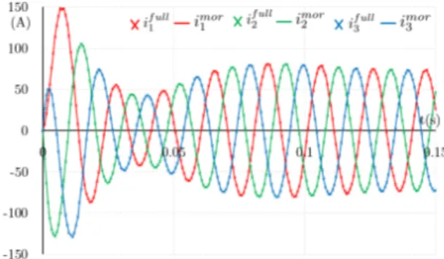
this reduced model, the both tests are recomputed with another time step fixed to 0.667ms in order to verify no loss of accuracy. Figures (3) and (4) present the evolution of currents for the test at synchronous speed and also the electromagnetic torque for the test at locked rotor obtained from the full and reduced models. For the two tests, the solutions obtained from the reduced model are close to the ones obtained by the full FE model. The average of the relative error εX is 2.27 · 10−3
and 5.4 · 10−3for the two tests and the speed up is about 15.
IV. SIMULATION FOR DIFFERENT OPERATING POINTS
A. Characteristic of the average electromagnetic torque versus the rotation speed
From the full and reduced models, we seek to determine the average electromagnetic torque Γav,emin function of the
speed Ω. Both models are solved for different values of fixed rotation speed. Figure (5) presents the evolution of Γav,em
versus Ω. The torque characteristics obtained from the models are very close for Ω > 80rad/s. For low rotation speeds, the difference is more significant but remain acceptable. In
Fig. 3. Evolution of currents from the full and reduced models for the test at the synchronous speed.
Fig. 4. Evolution of the electromagnetic torque from the full and reduced models for the test at locked rotor.
Fig. 5. Evolution of the average electromagnetic torque versus the rotation speed from the full and reduced models.
order to verify the efficiency of the reduced model, global and local quantities obtained from both models are compared for a fixed rotation speed equal to 141rad/s. Figures (6) and (7) present the evolution of the currents and of the Joule losses respectively. The global quantities obtained from the reduced model are similar to those from the full model. Figures (8) and (9) present the magnetic flux density in the stator and the eddy current density in the squirrel cage at the end of the time interval obtained from the reduced model. For each local quantity, the difference of results between both models is presented. For both cases, the magnitudes of the error are small compared with those of the magnetic flux density and of the eddy current density. The maximum of the error for B is located at the tip of the teeth. Then, the reduced model is valid to approximate the field distributions for any speed slip.
Fig. 6. Evolution of the currents from the full and reduced model.
Fig. 7. Evolution of the Joule losses from the full and reduced models.
Fig. 8. Magnetic flux density (T ) from the reduced model and error in the stator.
Fig. 9. Magnitude of the eddy current density (A/m2) from the reduced
model and error in the squirrel cage.
B. Study of the start-up for different load torques
From the reduced model defined by (13)-(15) coupled with (12), we study the start-up of the induction machine for two load torques. For the case 1, the torque Γr,1 is fixed to a
constant value equal to 20N m. For the case 2, the torque Γr,2 is defined as a quadratic function of the rotation speed
such as Γr,2 = 0.002Ω2. Figure (10) presents the evolution
of Ω for both cases. For the case 1, Γr,1 is close to the
starting torque (Fig. 5). A phase-shift appears between the evolutions of the speed Ω1obtained from the full and reduced
models. The dynamic of the speed up is directly related to the
difference ∆Γ between the electromagnetic and load torques. As observed in the section IV-A, at low rotation speeds, there is a gap of several percent between the electromagnetic torques given by the reduced and full models. Since the load torque is close to the starting electromagnetic torque, the gap between ∆Γ given by the reduced model and by the full model will be of several dozen percent at low speed which explains the difference of speed response. Nevertheless, the evolutions of the speed obtained from both models are similar. For the case 2, Γr,2is defined as a quadratic function of the rotation speed.
So at low speed, Γr,2is small leading to a gap of ∆Γ between
the reduced model and the full model small as well. In this condition, we can verify that the time evolutions of the speed Ω2 obtained from the full and reduced models are close.
Fig. 10. Evolution of the rotation speed for the two different load torques.
V. CONCLUSION
A reduced model of a squirrel cage induction machine based on the POD approach has been developed. Based on typical tests, a reduced basis is defined in order to build a reduced model valid on the whole operating range with a good compromise between accuracy and computational time compared with the full model. The effectiveness of the approach have been shown by simulating the stard up with two different load torque characteristics. Based on the proposed approach, accounting for the nonlinear magnetic behavior will be investigated in a future work.
REFERENCES
[1] J. Lumley, ”The structure of inhomogeneous turbulence”, Atmospheric Turbulence and Wave Propagation, A.M. Yaglom and V.I. Tatarski., pp. 221-227, 1967.
[2] T. Henneron and S. Cl´enet, ”Model-Order Reduction of Multiple-Input Non-Linear Systems Based on POD and DEI Methods”, IEEE Trans. Magn., vol. 51, no. 3, pp. 1-4, March 2015.
[3] L. Montier, T. Henneron, S. Clenet and B. Goursaud, ”Transient sim-ulation of an electrical rotating machine achieved through model order reduction”, Advanced Modeling and Simulation in Engineering Sciences, vol. 3, no. 1, 2016.
[4] J. Cheaytani, A. Benabou, A. Tounzi and M. Dessoude, ”Stray Load Losses Analysis of Cage Induction Motor Using 3-D Finite-Element Method With External Circuit Coupling”, IEEE Trans. Magn., vol. 53, no. 6, pp. 1-4, June 2017.
[5] T. Henneron, S. Cl´enet and F. Piriou, ”Calculation of extra copper losses with imposed current magnetodynamic formulations,” IEEE Trans. Magn., vol. 42, no. 4, pp. 767-770, April 2006.
[6] G. Krebs, T. Henneron, S. Cl´enet and Y. Le Bihan, ”Overlapping Finite Elements Used to Connect Non-Conforming Meshes in 3-D With a Vector Potential Formulation”, IEEE Trans. Magn., vol. 47, no. 5, pp. 1218-1221, May 2011