Analyzing Trade Liberalization Effect in the Egg Sector Using a Dynamic Gravity Model

(1)

Centre de Recherche en économie de l’Environnement, de l’Agroalimentaire, des Transports et de l’Énergie

Center for Research on the economics of the Environment, Agri-food, Transports and Energy

_______________________

Tamini : Corresponding author. CREATE, Université Laval, Pavillon Paul-Comtois, 2425, rue de l’Agriculture, local 4412, Québec (QC)

Canada G1V 0A6

lota.tamini@eac.ulaval.ca

Doyon : CREATE, Université Laval Simon : CREATE, Université Laval

Les cahiers de recherche du CREATE ne font pas l’objet d’un processus d’évaluation par les pairs/CREATE working papers do not undergo a peer review process.

ISSN 1927-5544

Analyzing Trade Liberalization Effect in the Egg Sector

Using a Dynamic Gravity Model

Lota D. Tamini

Maurice Doyon

Rodrigue Simon

Cahier de recherche/Working Paper 2012-6

(2)

Abstract:

This study analyzes the effects of different liberalization scenarios in the international trade of eggs and egg products. We use a dynamic gravity model that takes into account the observed persistence of trading partners. The estimated parameters of the gravity model serve to quantify the impact of various liberalization scenarios on the probability of importing (extensive margin) and on trade volumes (intensive margin). The results indicate that even in the context of aggressive trade liberalization, trade gains at the extensive margin will be modest. Gains at the intensive margin of trade are present even in the context of partial liberalization - Doha type - of trade.

Keywords: Eggs and eggs products, Persistence in trade, Trade liberalization, Gravity model,

Random-effects dynamic Probit, Autoregressive panel

Résumé:

Cette étude analyse les impacts de différents scénarios de libéralisation du commerce international des œufs, des ovoproduits et des produits à base d’œufs. Nous utilisons un modèle de gravité dynamique prenant en compte l’effet de persistance des partenaires commerciaux. Les paramètres estimés du modèle de gravité sont utilisés afin de quantifier l’impact des scénarios de libéralisation sur la probabilité d’exporter (marge extensive) et sur l’intensité des volumes commerciaux (marge intensive). Les résultats montrent que les gains sur la probabilité d’exporter sont modestes et cela quel que soit l’ampleur de la libéralisation des échanges. Par contre la libéralisation des échanges se traduit par une augmentation des volumes exportés aussi bien dans le cas du scénario de libéralisation partielle - type Doha - que dans celui d’une libéralisation agressive des échanges.

Mots clés: Œufs et ovoproduits, Persistance des flux commerciaux, Libéralisation du commerce,

Modèle de gravité, Probit dynamique à effet aléatoire, Panel autorégressif

(3)

1 Introduction

Despite broad globalization pressures, import tari¤s in agricultural and food industries remain particularly high compared with the industrial sector. The Organization for Economic and Co-operation Development (OECD) estimated that the average tari¤ for agricultural and agri-food products in OECD countries was 36% (OECD, 2003). The peaks of agricultural tari¤s are also a cause for concern. Bchir et al. (2005, p. 21) show that the shares of products with an average bound tari¤ in excess of 100% are 5.8% and 12.1% for developed and developing countries, respectively, but there is much variation between countries. Anderson (2009) provides a detailed account of the evolution of agricultural distortions in di¤erent parts of the world. Domestic support policies (e.g. input and output price subsidies) are ubiquitous in agriculture; their reduction represents one of the greatest challenges in the current round of WTO negotiations.1

The World Trade Organization’s (WTO) 2004 trade report shows a major structural change in the composition of agricultural trade, with trade in processed products growing more rapidly and surpassing trade in primary agricultural goods. This trend is observed across countries and agricultural product groups in spite of evidence of tari¤ escalation (Elamin and Khaira, 2003). In addition, data on international trade of agricultural products shows that there is persistence in trading partners. First, data features indicate that a large majority of partners do not trade with one another. Second, the growth of trade was due more to the growth of the volume of trade among countries with each other than to trade with new partners.

These features of agricultural trade are consistent with the recent work of Meltiz (2003), Chaney (2008) and Helpman, Melitz and Rubinstein (2008) implying that exports to a given destination incur a …xed cost and variable cost. The …rst cost justi…es the phenomenon of learn-ing by …rms historically active in the markets, and gives them an advantage over potential new entrants. Nonetheless, other variables in the gravity models (proximity, bilateral agreements, etc..) can explain the phenomenon of persistence of trade ‡ows. De Benedictis and Vicarelli (2005) speak of “inertia in trade ‡ows.” Kandilov and Zheng (2011) show that sunk costs are economically and statistically important for trade in major agricultural commodities even if access to export markets has improved in the years following the Uruguay Round. Taking per-sistence into account, Olivero and Yotov (2012) suggest a dynamic gravity equation based on capital accumulation. The authors introduce a term that encompasses two intuitive elements: a trade persistence e¤ect and a protection persistence e¤ect. The protection persistence e¤ect

1_{Uruguay Round negotiations resulted in an agreement on agriculture; one of the basics was the conversion}

of all non-tari¤ barriers (including QRs) into tari¤ equivalents. This was done to ensure that the pricing of trade barriers is not completely protectionist, hence the introduction of a combination system of tari¤ and quota (TRQ). This allows the entry of a limited amount of products at a low price. The quantities that exceed the minimum provided are subject to a very high, even prohibitive, rate. In Canada, this mechanism is e¤ective for several agricultural products: milk, poultry, hatching eggs and table eggs.

(4)

accounts for the fact that, because of domestic capital accumulation, trade barriers can lead to an increase in trade ‡ow through a positive e¤ect on output and country size. Olivero and Yotov’s main conclusion (2012: p. 3) is that “persistence in trade ‡ows should be accounted for by including lagged trade regressor in gravity models.”However, Olivero and Yotov’s approach does not take into account …rms behavior or their entry into foreign markets, contrarily to the …rm heterogeneity model of Helpman et al. (2008). Following the seminal work of Melitz (2003), Helpman et al. (2008) assume that trade costs vary depending on the level of trade. They are also …xed, determining …rms’ability to export, and hence the extensive trade margin.2 Egger and Pfa¤ermayr (2011) follow HMR when specifying their structural gravity models with mar-ket entry dynamics. Their key assumption is that …rms consider the role of path dependence for market entry. The implication of this approach is that sunk entry costs are time-declining for …rms that are present in a given market.

The objective of the paper is therefore to explore potential change in trade induced by di¤erent liberalization scenarios when taking into account the phenomenon of persistence in trading partners. Our application focuses on the egg sector, where the persistence in trading partners is acute. Table eggs, eggs for processing (albumin and eggs not in shell) and egg products are analyzed to capture potential di¤erences in structural parameters by the type of eggs.

Our methodological approach is based on a gravity model.3 In its simplest form, the gravity equation explains trade volume by supply and demand factors (GDP and population), trade resistance factors (distance, tari¤s, etc.) and trade preference factors (common language and border, preferential trade agreements, etc.). As mentioned by De Benedictis and Vicarelli (2005:1) “its relative independence from (or ability to mirror) di¤erent theoretical models...have

2_{The impacts of …rms’heterogeneity on international trade are now well documented (see for example Bernard}

and Jensen, 1999). However, relatively few studies account for this feature when estimating gravity equations. Tamini, Gervais and Larue (2010) and Kandilov and Zheng (2011) are recent applications of the HMR framework to agricultural products.

3_{Rude and Gervais (2006) and Rafajlovic and Cardwell (2010) use a partial equilibrium model and numerical}

simulations when analyzing trade policy in the Canadian chicken sector. The advantage of this approach is that it is not too demanding in terms of modelling and data. However, it identi…es and analyzes very few variables in‡uencing international trade. Further, it is suitable for the analysis of the situation of only one country at a time. Computable general and partial equilibrium models are also common when studying the impacts of change in trade policies. This approach is demanding in terms of data: di¢ culties emerge when one tries to study a small sector of the economy like the egg sector. A recent example is Abassi, Bonroy and Gervais (2008), who use a partial equilibrium model in the Canadian dairy sector. Grant, Hertel and Rutherford (2009) extend this approach by associating partial equilibrium and general equilibrium models to analyze the impacts of liberalization of imports of specialty cheeses in the United States through the expansion of bilateral quotas. These approaches are data consuming, and depend on the structural parameters used to calibrate the model. The egg sector has very little information on such parameters, which limits the relevance of such approaches.

(5)

made the gravity model the empirical model of trade ‡ows.”4 Consistent with Vijay and Shahid (2011), we use a panel estimation approach to control for unobserved heterogeneity of trading partners. Given the inertia in trade ‡ow, we follow Kim et al. (2003), De Benedictis and Vicarelli (2005) and Campbell (2010) and use a panel dynamic model. Campbell (2010) shows that taking into account the dynamic nature of trade ‡ows also helps solve the puzzle of distance the elasticity of distance does not diminish over time (see also Disdier and Head, 2008).5 Because of zero trade ‡ows, estimations are done with a double correction, as suggested by Helpman et al. (2008).

Our estimations strongly support the panel dynamic speci…cation compared with the panel model without dynamic features. The dynamic speci…cation can therefore shed new light on the e¤ects of trade agreements. It can help explain why trade liberalizations often increase trade creation between countries that had already been trading partners. Using the estimated parameters, an aggressive liberalization and a Doha-type compromise outcome are simulated to assess the importance of extensive and intensive margin e¤ects of these trade liberalization scenarios. Overall, simulations indicate that our trade scenarios would result in an increase in the intensity of trade, but very few emerging trading partners (extensive margin). For the two liberalization scenarios, the impact is greater for eggs in shell.

The remainder of the paper is structured as follows. The next section presents the conceptual approach of the trade model underlining the implications of persistence in trading partners. The third section introduces the econometric procedure used to estimate the structural parameters of the model. The fourth section presents the estimation results, and section 5 analyzes various liberalization scenarios and their implications in the context of the current Doha Round. The last section concludes the paper.

2 A glance at the data

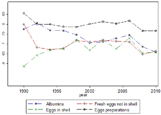
As mentioned, we analyze four products to capture di¤erences in structural parameters by level of transformation: Eggs in shell, Fresh eggs not in shell, Albumin and Egg preparations.

Figure 1 shows that about 70% of trade ‡ow in a given year is likely to be present in the next year. When considering a …ve-year interval, the mean of the persistence phenomenon is around 60%. More important, less than 1% of “zeros”are not zeros in the two following years, implying

4_{Applications of gravity models in the agricultural sector at the aggregated level include Paiva (2005) and}

Koo, Kennedy and Skripnitchenko (2006). Sarker and Jayasinghe (2007) and Susanto, Rosson and Adcock, (2007), Tamini, Gervais and Larue (2010) and Ghazalian et al. (2011) are recent applications at a disaggregated level.

5_{This is important for international trade of table eggs because they are mainly a convenience store product,}

at least with respect to eggs in shell. Available at http://www.agr.gc.ca/poultry/ prinde2_fra.htm#sec27. Accessed August 17, 2011).

(6)

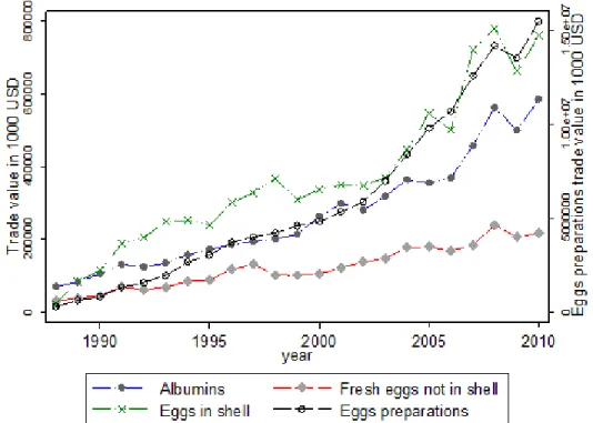
“incapacity” in creating new trade ‡ows. Figure 2 shows that a small proportion of countries trade in both directions. The exception is egg preparations, where trade in both directions is present in about 50 of trading partners. Disregarding theses features could result in selection and/or asymmetry bias.

Despite this inertia in trading relationships, Figure 3 indicates that at the end of the period, the aggregate trade value was about 32 times larger than the aggregate trade value of the beginning of the period. Combining Figure 1-4 suggests that the growth in world trade must have been much larger due to the increase in the volume of existing bilateral trade.

The …nding of Kandilov and Zheng (2011) that market access improved in the years following the Uruguay Round seems to be refuted in the egg industry. Figures 5-6 show a very slow decrease in the average applied ad valorem tari¤s.

3 Theoretical model

The theoretical model draws from the framework developed by Anderson and van Wincoop (2003). Assume that there are Z (z = 1; :::; i; j:::; Z) countries with consumers endowed with identical preferences over consumption. Consumers’ preferences are captured by a CES-type utility function over varieties. Let qi(!) be country i’s consumption of one product variety with

indexing varieties. The parameter measures the elasticity of substitution between varieties and hence > 1. The utility function in country i is: :

Ui = Z !2 qi(!)( 1)= =( 1) (1) where i is the set of variables available in country i.

Each …rm within a country produces a di¤erent variety, with Nj. being the (…xed) number

of varieties in country j Assume that the technology for production in country j can be rep-resented by a constant returns to scale Cobb-Douglas production function: T F Pj(!) IjK

1

j ;

where T F Pj(!) is a total factor productivity index speci…c to a …rm in country j, Ij and Kj,

respectively, denote speci…c input and capital used in production and the speci…c input cost share. The speci…c input and capital factor prices are denoted by hj and rj, respectively and are

perceived to be constant. Under these assumptions, the marginal cost is: cj = $j(!) rj1 hj,

where $j(!) (1 ) (1 )( ) =T F Pj(!). The variable $j(!) is a …rm-speci…c

pro-ductivity parameter with country-speci…c support $j(!)2 $j; $j :6

6_{Following Helpman et al. (2008), it is assumed that the distribution function of $ is identical across}

(7)

Pro…t maximisation implies:

pi=si = ( 1) 1cj (2)

where pj is the price received by …rms in country j and sj represents prices and distorting

domestic support policies in country j with .sj < 1

From the consumers’standpoint, two-stage budgeting allows for conditional expenditures on varieties. The e¤ective price paid by consumers for a given variety is pj multiplied by net trade

costs tij between countries i and j. Using (2), the country i’s demand function for a variety

supplied by country j is as in Feenstra (2004:152-153):

qij = Yi (tijcj) P z(tizcz) 1 Nz (3) where Yi represents income in country i and tij as de…ned before. We follow Helpman et

al. (2008) and assume that only a fraction of …rms in country j , (Vj)export to a particular

destination i. This fraction is determined by a threshold productivity shock de…ned by the existence of a destination-speci…c …xed export cost. Firms will export to a destination if they earn positive pro…ts. Assumptions about productivity and the existence of …xed export costs imply that only a fraction of …rms export to a particular destination. Country i’s imports from j are equal to the consumption of each variety de…ned in (3) multiplied by the fraction (Vj) of

the number of varieties (Nj) that are exported, thus capturing the impact of the …rm-speci…c

productivity shock. We can write total imports as:

Mij = VijNjqij = Yi (tijcj) VijNj P z(tizcz) 1 Nz (4) For future reference, we de…ne the relationship between egg production in country j (denoted Qj) and the total demand faced by country j by:

Mij = Mij= X z Mzj ! Qj (5)

Substituting the import demand function in (4) for on the right-hand side of (5) yields:

Mij = j1Yi (tijcj) P z(tizcz)1 Nz VijNjQj (6) where . j P_zYiP(tijcj) VijNj z(tizcz)1 Nz.

Equation (6) combines the intensive and extensive margins of trade (See Helpman et al., 2008).

(8)

4 Empirical framework

In our empirical approach we estimate a dynamic type 2 Tobit model.

4.1 Trade intensity

The log-linearization of equation (6) yields the following equation to be estimated:

ln Mij;t = ln Yi+ ln Vij + ln Nj;tQj;t ln tij+ i;t+ i;t+ vij;t (7)

where j ln (cj) ln j and j ln P_z(tizcz)1 Nz are exporter and importer

…xed e¤ects respectively, and the other variables de…ned before. Following Egger (2002) dy-namics is introduced into as static regression via an autoregressive AR (L) error term: ij;t =

+

L

P

`=1

` ij;t ` + "ij;t with j j < 1:This assumption implies that Cov [ ij;t; ij;t `] 6= 0. This

model can also be written as an auto-regressive distributed-lag model of the form:

ln Mij;t = L X `=1 `ln Mij;t `+ xij;t+ L X `=1 ` xij;t `+ "ij;t (8)

where xij;t ln Yi + ln Vij + ln Nj;tQj;t ln tij + i;t + i;t:Given this speci…cation the

coe¢ cients summarized by the vector represent the short term impact of the variables of the gravity equation while

L

P

`=1 `

represent the long term impact.

4.2 Selling in a foreign market: dynamic persistence and …xed e¤ects

Following Melitz (2003), we consider that selling in a given foreign market implies that …rms must pay some …xed costs. While all …rms in country j sell output domestically, only a fraction of …rms sell abroad. The ability to export is conditional on the …rm-speci…c productivity factor. Using a zero pro…t condition, we de…ne a latent variable Eij as the ratio of the pro…t of country

j’s most productive …rm to the …xed costs (common to all exporters) when exporting to country i..7 _{A …rm’s self-selection into country i’s export market is observed if and only if E}

ij > 1. Fixed

trade costs are assumed to be stochastic and i.i.d. The latent variable can be expressed as: ln Eij = 0+ j+ i+ 1tij + ij (9)

where 0 is a constant term, 1 (1 ), j (1 ) ln (pj) j is the exporter …xed

e¤ect,8

i ln i+ ln Yi i is the importer …xed e¤ect, trade costs are de…ned by t and

7_{For details see Helpam et al. (2008) and the applications of Tamini et al (2010) and Kandilov and Zheng}

(2011).

8_{Feenstra (2004) argues that …xed e¤ects are appropriate to estimate the average impact of the border barriers}

(9)

is a random error term.

Following Das, Robert and Tybout (2007) and Segura-Cayuela and Vilarrubia (2008) we assume that there are three costs that …rms need to incur when selling to export markets. The …rst ones are iceberg variable trade costs. The second cost is a onetime sunk cost to access the foreign market. The third one is a …xed per-period cost assumed to be i.i.d. distributed. As mentioned by Segura-Cayuela and Vilarrubia (2008) one possible interpretation of the onetime sunk cost is the adaptation of …rms’production structure, while the …xed cost represents the cost of distribution or of sustaining a position in a given market. Das et al. (2007) assert that sunk costs are start-up costs of establishing distribution channels, learning bureaucratic procedures, and adapting their products and packaging for foreign markets. These assumptions imply that …rms will enter a foreign market only if they expect per-period revenues large enough to cover sunk and …xed costs. When it stops exporting, the …rm saves the per-period …xed cost. The latent variable eij;t ln Eij;t of equation (9) is then:

e_ij;t = eij;t 1+ 0wij;t+ ij + ij;t (10)

Equation (10) is the selection equation that determines the existence of trade ‡ow. It is a function of past selection outcome eij;t 1, strictly exogenous variables wij;t and time-invariant

unobserved individual e¤ect _ij. The scalar captures the e¤ect of past selection outcome, and the vector the e¤ect of explanatory variables on the current process. The current selection outcome is de…ned as:

eij;t= 1 eij;t > 0 (11)

Where 1 [:::] is the indicator function with value one if the expression between square brackets is true and zero otherwise. Trade is observed only if e_ij;t> 1:

mij;t = 1 eij;t> 0 mij;t (12)

where mij;t is a latent dependant variable.

4.3 Trade costs

The trade costs include the import tari¤ (denoted by ij 1), the e¤ect of distance summarized

by dij with dij = dji, the e¤ect of some factual factors of trade preference (trade agreement,

common language and borders,...) summarized by ij and …nally sj represents prices and

distorting domestic support policies as de…ned above. In our database, some countries have import quotas. We take this into account by adding dummy variables representing the fact that importer and/or exporter engage in supply management in the egg sector.

(10)

Trade costs that subsume net trade costs and domestic policies are de…ned as: etij = sejs e ijd ed ij ij (13) with ij = exp

# ₁languageij + # 2borderij + # 3GAT Ti+ # 4GAT Tj

+# ₅RT Aij+ # 6quotai+ # 7quotaj + # 8legalij

!

: (14) We assume that factual factors of trade preference summarized by ij have an impact on

the probability to trade but do not have and impact on the intensity of trade. Trade cost used for the gravity equation is then:

etij = sejs e ij d

ed

ij: (15)

4.4 Estimation strategy: addressing the initial condition problem

Estimations are done using a dynamic random e¤ect Probit model. The presence of omitted individual heterogeneity, in the form of individual-speci…c e¤ects in the …rst period, causes an “initial conditions” problem and renders the standard random-e¤ects (RE) probit estimator inconsistent when T (time lenght) is small. We use the two-step Heckman (1979) estimators as proposed by Stewart (2007) and Arulampalam and Stewart (2009).9 _{Estimations are done}

using Maximum simulated likelihood (Stewart, 2006).

In the second stage (trade intensity), estimations are done using double correction as pro-posed by Helpman et al. (2008: p 456) to deal with heterogeneity at the …rm level. A polynomial decomposition of the selection variable is used to correct for the bias associated with …rm hetero-geneity. Finally, to control for the possibility of tari¤s being endogenous, we use as instruments the lagged value of tari¤s and the three-year lagged moving average mean of the value of trade and the production of the country of origin of the trade ‡ow. The underlying intuition is that stronger import competition from a country is more like to trigger protection (see Debaere and Mostashari, 2010; Olivero and Yotov, 2012).10

9_{Alternative estimation methods to solve the initial conditions problem are proposed by Orme (1997, 2001),}

and Wooldridge (2005).

10_{The Wald tests for exogeneity con…rmed concerns about endogeneity of tari¤s, especially for eggs in shell}

(11)

5 Data sources

Trade volumes were obtained from the UNCOMTRADE database. Trade policies were col-lected from the TRAINS dataset; they account for preferential trade agreements between coun-tries/regions.11 _{The domestic support measure is taken from the WTO database, and re‡ects}

compilation of various (trade-distorting) domestic support measures, converted to ad valorem equivalent rates.12 _{It avoids possible double counting, particularly when domestic policies are}

combined with border policies (as in the case of administered prices).

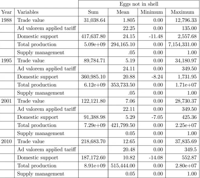
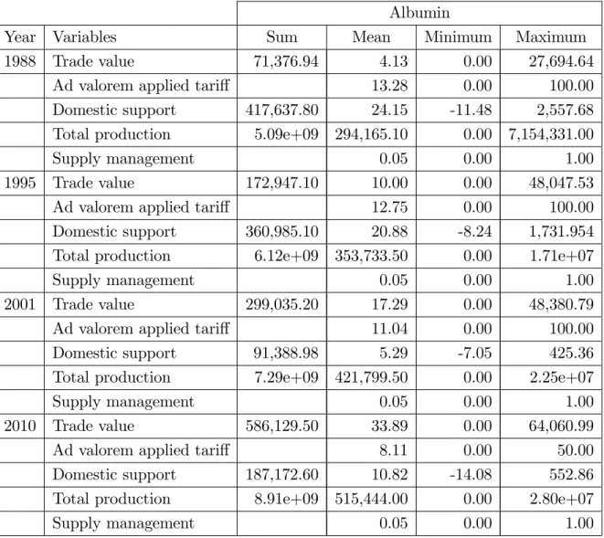
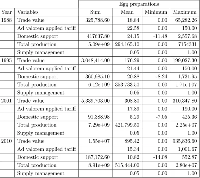
Total egg production is collected from the Food and Agriculture Organisation (FAO) Statis-tical Yearbook. Gross Domestic Product (GDP) statistics are collected from the International Monetary Fund (IMF) World Economic Outlook Database. The dataset of distances, other trade preferences and trade resistance factors is based on a compilation by the Centre d’Études Prospectives et d’Informations Internationales (CEPII). We use the harmonic distance measure as in Head and Mayer (2002). Adjusting for missing and outlier data resulted in a dataset of 132 countries/regions,13 _{listed in the appendix (Table A1). Table 1 presents descriptive statistics of}

the variables of interest.

6 Estimation results

6.1 Dynamic probit estimates

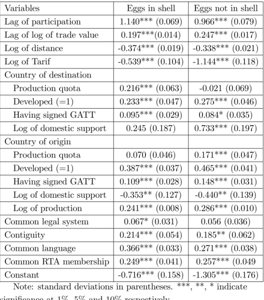
We estimate the total sample and split it into three distinct time periods based on WTO free trade negotiation rounds to check if market access has changed during and after the negotia-tions. The …rst period includes the Uruguay Round, which started in 1988 and ended in 1994. The second period includes the years 1995 to 2000 until the beginning of the Doha Round ne-gotiations. The last period, from 2001 to 2010, includes 10 years of the current Doha Round negotiations. Table 2 reports the estimated results for the last period of our dynamic Probit estimation of equation (10).14

For eggs in shell, as expected, the estimated coe¢ cient for distance is found to be higher than that for the other products. The likelihood of importing is higher when the two trading

11_{Data on trade and tari¤s were collected using World Integrated Trade Solution (WITS) software developed}

by the World Bank, in collaboration and consultation with various International Organizations including the United Nations Conference on Trade and Development (UNCTAD), International Trade Center (ITC), United Nations Statistical Division (UNSD) and World Trade Organization. (See http://wits.worldbank.org/wits/)

12_{The dataset is built using WTO member noti…cations, and is restricted to policies classi…ed as}

trade-distorting.

13_{European Union comprises 27 member nations.}

14_{We present the last period results only, because of space constraints. The detailed results of all periods are}

(12)

partners are developed countries indicating that it is easier for them to overcome …xed costs. The impact of the exporter’s domestic agricultural production is expected to be positive, while the importer’s domestic agricultural production is expected to reduce the probability of non-zero trade ‡ows. Our results con…rm our expectations and are in line of those of Ghazalian, Larue and Gervais (2009) and Kandilov and Zheng (2011).

We assess the impact of the history of export market participation proxied by the lagged value of participation. The results are both economically and statistically signi…cant for all products. The impact is higher for eggs in shell, as expected, followed by egg products (albumin and eggs not in shell) and …nally egg preparations.15 The estimate (not presented here) shows that for eggs in shell the value is relatively stable, from 2.24 in the …rst period to 2.22 in the last period, although it declines over time for the other products. The same is observed for the impact of distance on the extensive trade margin.

Marginal e¤ect of market entry sunk cost We follow Kandilov and Zheng (2011) and com-pute the marginal e¤ect of market entry sunk cost as Pr [eij;t= 1jeij;t 1= 1] Pr [eij;t = 1jeij;t 1 = 0].

The standard error is computed using the bootstrapping methods proposed by Krinsky and Robb (1986). The di¤erence between the two values indicates how entry costs reduce the probability of exporters’participating in foreign markets. The results are summarized in Table 3.

As expected, the negative impact of sunk costs on the probability of export market partic-ipation di¤ers substantially across commodities. The impact of sunk costs is smaller for egg products, while it is larger for Eggs in shell and Egg preparations.

Consider now the temporal pattern of the impact of entry costs on export market participa-tion. For Eggs in shell, the e¤ect of sunk costs increases from the …rst period to the second, and remains unchanged in the last period. The same result was found by Kandilov and Zheng (2011) for cereals, meat and dairy products in developing countries. For Eggs not in shell, Albumin and Egg preparations, the e¤ect of sunk costs decreases over the three periods. This …nding is in line with Kandilov and Zheng (2011), who report that in general, market access was improved by the Uruguay Round. Debaere and Mostashiri (2010) also found that reduction of tari¤s had an impact statistically signi…cant on the extensive margin of trade. Finally, the impact of sunk costs on the probability of export market participation is higher when the destination market is a developed country.

15_{Because in our speci…cation e}

ij;t is a function of eij;t 1 and not of eij;t 1, the fact that some coe¢ cients are

greater than 1 is not an issue. Kandilov and Zheng (2011) found a coe¢ cient greater than 1% in about 10% of their estimations for aggregate products.

(13)

6.2 Intensity of trade

As indicated in Table 4, a positive and highly signi…cant autocorrelation coe¢ cient clearly points out the importance of dynamics for the four products. The coe¢ cient on distance is always negative and signi…cant at the 5% level. As expected, there is a di¤erence between goods with a higher impact for Eggs in shell and Egg preparations. The e¤ect of importer GDP per capita, which serves as a proxy for foreign market demand, is positive when signi…cant. This result con…rms the intuition that greater revenue increases consumption of eggs and egg products. The future increase in the revenue of developing countries is thus expected to boost the probability of trade in the egg sector. Yet for Eggs in shell and Eggs not in shell the coe¢ cient is not signi…cant. As expected, total production of country of origin has a positive impact on the level of trade. Finally tari¤s have an expected negative impact on the level of trade of Eggs in shell and Egg preparations, with a higher impact for the …rst product. For Albumin and Eggs not in shell our results show that tari¤s do not a¤ect the intensity of trade. These results con…rm Figures 5-6 and 3-4, which indicate an increase in global trade despite a minor reduction in tari¤s coupled with a stable value of the mean of bilateral trade ‡ows. For these two products, the growth in trade mainly concerned the extensive trade margin.

7 Impulse response to change in trade policies

In this section we investigate the changes in intensive and extensive margins following two liberalization scenarios. The …rst one is an aggressive liberalization scenario, which eliminates all import tari¤s and domestic support.

The second liberalisation scenario depicts a potential Doha “compromise” outcome. It in-volves removing export subsidies and cutting trade-distorting domestic policies according to the level of global support: 80 percent for the European Union, 70 percent for the United States and Japan and 55 percent for the other countries. The extent of tari¤ cuts depends on whether protection is implemented through a Tari¤-Rate Quota (TRQ) or a simple tari¤. In most cases, TRQs act as de facto import quotas because they set a minimum level under which imports are taxed at a very low (often zero) rate. Any imports above the minimum access are taxed at a very high (often prohibitive) rate. The moderate liberalization scenario includes tari¤ cuts of 20 percent when imports are restricted by a TRQ. The implicit assumption is that egg products currently protected by a TRQ are likely to be designated as sensitive, a notion introduced in the Doha Framework Agreement (WTO, 2008) and thus warrant distinct tari¤ cuts. For developed countries, “the moderate liberalization”scenario also includes tari¤ cuts of 70 percent if initial tari¤s are higher than 75 percent and 50 percent in all other instances. For developing countries the tari¤s is 50 percent in all instances. Note that neither scenario entails full liberalization, which would require addressing non-tari¤ barriers to trade.

(14)

The impact of the liberalization processes re‡ects adjustments on two margins: extensive and intensive margin, both within a dynamic setting. To quantify each type of response we simulate imports’reactions to a permanent change that took place in period 1, and track the evolution of the probability to export and the trade during the next 10 periods. The year 2010 was set to be period 1. For a given period when an estimated probability of exporting is strictly higher than 0.5, we consider that trade occurs. If the probability of exporting is lower than or equal to 0.5, we consider that trade does not occur during this period. Because the estimated parameters of tari¤s are non-signi…cant statistically for Albumin and Eggs not in shell, the following analyses are done for Eggs in shell and Egg preparations using the estimation results of the 2001-2010 period.

7.1 Extensive margin of trade

Trade liberalisation would induce a small increase in the probability of non-zero trade. Under the aggressive liberalization scenario, the increase in the average probability over the entire sample is less than ten percent for Egg preparations while it is higher at 80% for eggs in shell (See Figures A1 and A2). For the two scenarios, the probabilities of exporting are higher, but most of countries do not exceed the threshold of 0.5 at the end of the 10 periods examined. These results were also found by Debaere and Mostashiri (2010) for the vast majority of analyzed products. The authors also found disparity between products and between developed and developing countries. Debaere and Mostashiri (2010: 168) concluded that “ At best, ... 12% of newly traded goods can be attributed to tari¤ reductions. ... This indicates that other factors at both the industry and country levels play a much more signi…cant role in explaining changes in the extensive margin.”

7.2 Intensive margin of trade

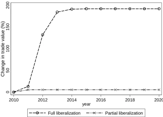
As indicated by Figure 7, the aggressive liberalization induces an increase in the intensive margin of trade of eggs in shell of about 200%. It is reached three years after aggressive liberalization. We thus observe a contemporaneous response and ampli…ed e¤ects through dynamic adjustments at the intensive margin.16 Figure 7 illustrates that the biggest marginal response occurs in the second period. In the partial liberalization scenario the full gain is obtained after the …rst period, implying a very small dynamic adjustment.

Figure 8 depicts the impact of the two liberalization scenarios on international trade of Egg preparations. The dynamic e¤ect is smalter, corresponding to a gain in trade of about

16_{There is also dynamic adjustment at the extensive margin. However, as mentioned, it applies to very few}

(15)

150% following full liberalization, after …ve periods. The increase in trade following partial liberalization is modest.

Figures A3-A6 indicate the same feature when considering developed countries and Canadian imports. For developed countries’imports from developing countries and for Canadian imports the biggest marginal response occurs at the beginning of the period, indicating the trigger e¤ect of the high level of tari¤s.

8 Conclusions

Trade in processed products is growing more rapidly, and becoming more important than trade in primary goods. This trend is observed across countries and product groups, despite evidence of tari¤ escalation and considerable heterogeneity in domestic support policy reduction between countries. In addition, a large majority of partners do not trade with one another, suggesting that the growth of trade was predominantly due to the growth of the volume of trade among countries that trade with each other. Moreover, …rms historically active in the markets would have an advantage (knowledge) over potential new entrants.

Therefore in this paper we explored potential changes in trade induced by di¤erent liberal-ization scenarios, taking into account the phenomenon of persistence in trading partners. Our application focuses on the egg sector, where the persistence in trading partners is acute. Over 94% of the trading partners in 2000 were still partners in 2008, whereas less than 6% of the partners of 2008 were not trading with one another in 2000. The dataset covers the period from 1988 to 2010. Table eggs, eggs for processing (Eggs not in shell and albumin) and egg products were analyzed to capture potential di¤erences in structural parameters by the type of eggs. Our methodological approach is based on a gravity model estimated using dynamic panel econometrics. We thus take into account the persistence of trading partners while controlling for unobserved heterogeneity of bilateral trading partners. We correct for the “zeros” in trade ‡ows using the sample selection approach suggested by Helpman et al. (2008).

Our estimations strongly support the panel dynamic speci…cation. The dynamic speci…ca-tion can therefore shed new light on the e¤ect of trade agreements. It can help explain why trade liberalization often leads to relatively larger trade creation between countries that were previously trading partners. For eggs in shell the estimated coe¢ cient for distance on the ex-tensive margin of trade is found to be higher than that for the other products. The likelihood of importing is higher when the two trading partners are developed countries indicating that it is easier for them to overcome …xed costs. The impact of the exporter’s domestic agricultural production is expected to be positive, while the importer’s domestic agricultural production is expected to reduce the probability of non-zero trade ‡ows.

(16)

Using the estimated parameters, aggressive liberalization and Doha-type compromise out-comes were simulated to assess the importance of extensive and intensive margin e¤ects of these trade liberalization scenarios studied. Overall, simulations indicate that our trade scenarios would intensify of trade, but not increase trading partners noticeably (extensive margin). For the two liberalization scenarios, the impact (in percent of increase) is greatest for eggs in shell.

(17)

Bibliography

Abbassi, A., Bonroy, O and Gervais, J.P. 2008. Dairy Trade Liberalization Im-pacts in Canada. Canadian Journal of Agricultural Economics 56: 313-335.

Anderson, K. 2009. Distortions to Agricultural Incentives: A Global Perspective, 1955-2007 (Washington, DC: The World Bank).

Anderson, J. E. and van Wincoop, E. 2003. Gravity with Gravitas: a Solution to the Border Puzzle. American Economic Review 93: 170-192.

Arulampalam, W. and Stewart, M.B.2009. Simpli…ed Implementation of the Heckman Estimator of the Dynamic Probit Model and a Comparison with Alternatives Estimators. Oxford Bulletin of Economics and Statistics 71: 659-681.

Bchir, M.H., Jean, S. and Laborde, D. 2005. Binding overhang and Tari¤ cutting Formulas. CEPII Working Paper 18, Paris, France.

Bernard, A. B. and Jensen, J. B. 1999. Exceptional Exporter Performance: Cause, E¤ect, or both? Journal of International Economics 47: 1–25.

Campbell, D. L.2010. History, Culture, and Trade: a Dynamic Gravity Approach. MPRA working paper.

Chaney, T.2008. Distorted Gravity: the Intensive and Extensive Margins of International Trade. American Economic Review 98: 1707-1721.

Das, M., Robert, M. and Tybout, J.R. 2003. Market Entry Costs, Producer Hetero-geneity and Export Dynamics. Econometrica 75: 837-873.

De Benedictis, L. and Vicarelli, C. 2005. Trade Potentials in Gravity Panel Models. Topics in Economic Analysis & Policy Volume 5, issue 1, article 20.

Debaere, P. and Mostashari, S. 2010. Do Tari¤s Matter for the Extensive Margin of International Trade? An Empirical Analysis. Journal of International Economics 81: 163–169. Disdier, A-C. and Head, K. 2008. The Puzzling Persistence of the Distance E¤ect on Bilateral Trade. The Review of Economics and Statistics 90: 37-48.

Egger, P. 2002. An Econometric View on the Estimation of Gravity Models and the Calculation of Trade Potentials. The World Economy 25: 297-312.

Egger, P. and Pfa¤ermayr, M. 2011. Structural Estimation of Gravity Models with Path-dependence Market Entry. CEPR Discussion Papers 8458.

Elamin, N. and Khaira, H.2003. Tari¤ Escalation in Agricultural Commodity Markets. FAO Commodity Market Review, 101-120. Rome, Italy.

Feenstra, R. C. 2004. Advanced International Trade. Theory and Evidence. Princeton and Oxford: Princeton University Press.

Ghazalian P., Larue B. and Gervais. J-P.2009. Exporting to New Destinations and the E¤ects of Tari¤s: The Case of Meat Commodities. Agricultural Economics 40: 701-714.

(18)

Gravity-based Framework when there are Vertical Linkages Between Markets with an Appli-cation to the Cattle/Beef Sector. Journal of International Trade and Economic Development. (DOI: 10.1080/09638199.2010.505297)

Grant, J.H., Hertel, T.W. and Rutherford, T.F. 2009. Dairy Tari¤-Quota Liberal-ization: Contrasting Bilateral and Most Favored Nation Reform Options. American Journal of Agricultural Economics 91: 673–684.

Heckman, J. J. 1979. Sample Selection Bias as a Speci…cation Error. Econometrica 47: 153-161.

Helpman, E., Melitz, M.J. and Rubinstein, Y.2008. Estimating Trade Flow: Trading Partners and Trading Volumes. Quarterly Journal of Economics 123: 444-487.

Kandilov, I.T. and Zheng X. 2011. The Impact of Entry Costs on Export Market Participation in Agriculture. Agricultural Economics 42: 531-546.

Kim, M., Cho, G. D., Koo, W.W. 2003. Determining Bilateral Patterns using a Dynamic Gravity Equation. Agribusiness & applied economics report 525. North Dakota University.

Koo, W.W., Kennedy, P.L. and Skripnitchenko, A. 2006. Regional Preferential Trade Agreements: Trade Creation and Diversion E¤ects. Review of Agricultural Economics 28: 408-415.

Krinsky, I and Robb, A.L. 1986. On Approximating the Statistical Properties of Elas-ticities. Revew of Economics and Statistics 68: 715-719.

Meltiz, M. J. 2003. The impact of Trade on Intra-industry Reallocations and Aggregate Industry Productivity. Econometrica 71: 1695-1725.

Olivero, M. P. and Yotov, Y.2012. Dynamic Gravity: Theory and Empirical Implica-tions. Canadian Journal of Economics 45: 64-92.

Orme, C.D. 1997. The Initial Conditions Problem and Two-Step Estimation in Discrete Panel Data Models. Mimeo, Department of Economic Studies, University of Manchester, UK. Unpublished paper.

Orme, C.D.2001. Two-step Inference in Dynamic non-linear Panel Data Models. School of Economic Studies, University of Manchester, mimeo, downloadable from: http://personalpages. manchester.ac.uk/sta¤/chris.orme/

OECD. 2003. The Doha Development Agenda: Welfare Gain from Further Multilateral Trade Liberalization with Respect to Tari¤s. Available at www.oecd.org/trade under Publica-tions and Documents/Reports (accessed 17 October 2011).

Paiva, C.2005. Assessing Protectionism and Subsidies in Agriculture: A Gravity Approach. International Monetary Fund (IMF) Working Paper No. 05/21, Washington, D.C.

Rafjalovic, J. and Cardwell, R. 2010. The Implication of WTO Negotiations on the Canadian Chicken Market: two Representations of Chicken and Stochastic World Prices.

(19)

CAPT-PRN working paper 2010-07

Rude, J. I. and Gervais J-P. 2006. Tari¤-rate Quota Liberalization: the Case of World price Uncertainty and Supply Management. Canadian Journal of Agricultural Economics 54: 33-54.

Sarker, R., and Jayasinghe, S.2007. Regional Trade Agreements and Trade in Agri-food Products: Evidence for the European Union from Gravity Modeling using Disaggregated Data. Agricultural Economics 37: 93-104.

Segura-Cayuela R. and Vilarrubia, J. M. 2008. Uncertainty and Entry into Export Markets. Banco de Espana Working Papers 0811, Banco de España

Stewart, M.B. 2007. The interrelated Dynamics of Unemployment and Low-wage Em-ployment. Journal of Applied Econometrics 22: 511-531.

Stewart, M. B. 2006. Maximum Simulated Likelihood Estimation of Random-e¤ects Dy-namic Probit Models with autocorrelated Errors. Stata Journal 6: 256-272.

Susanto, D., Rosson, C.P. and Adcock, F.J.2007. Trade Creation and Trade Diversion in the North American Free Trade Agreement: the Case of Agricultural Sector. Journal of Agricultural and Applied Economics 39: 121-134.

Tamini, L.D., Gervais, J-P. and Larue, B. 2010. Trade Liberalisation E¤ects on Agricultural Goods at Di¤erent Processing Stages. European Review of Agricultural Economics 37: 453-477.

Vijay K. V. and Shahid S. 2011. An Estimation of the Latent bilateral Trade between India and Pakistan using Panel Data Methods. Global Economic Review 40: 45-65.

Wooldridge, J. M.2005. Simple Solutions to the Initial Conditions Problem in Dynamic, nonlinear Panel Data Models with unobserved Heterogeneity. Journal of Applied Econometrics 20: 39–54.

Wooldridge, J. M. 2002. Econometric Analysis of Cross Section and Panel Data. Cam-bridge MA: MIT Press.

World Trade Organization. 2004. Word Trade Report. Exploring the Linkage Between the Domestic Policy Environment and International Trade. Available at: www.wto.org/english /res_e/reser_e/wtr_arc_e.htm. Accessed February 3, 2012.

World Trade Organization. 2008. Committee on agriculture special session. Revised draft modalities for agriculture. www.wto.org/english/tratop_e/agric_e/agchairtxt_july08_ e.pdf. Accessed March 31, 2012.

(20)

List of …gures

Figure 1. Fraction of positive trade ‡ow during two successive years

(21)

Figure 3. Aggregate volume of export of all countries (x 1 000 US$)

(22)

Figure 5. Evolution of tari¤s in %

(23)

0 50 1 00 1 50 2 00 Cha ng e in tra de val u e ( %) 2010 2012 2014 2016 2018 2020 year

Full liberalization Partial liberalization

Figure 7. Cumulative impact on the value of trade of eggs in shell

0 50 1 00 1 50 Cha ng e in tra de val u e ( %) 2010 2012 2014 2016 2018 2020 year

(24)

List of tables

Table 1. Summary statistics of the data used in estimations Eggs in shell

Year Variables Sum Mean Minimum Maximum

1988 Trade value 24,012.71 1.38 0.00 19,519.74 Ad valorem applied tari¤ 20.44 0.00 230.00 Domestic support 417,637.80 24.15 -11.48 2,557.68 Total production 5.09e+09 294,165.10 0.00 7,154,331.00

Supply management 0.05 0.00 1.00

1995 Trade value 238,963.20 13.82 0.00 35,373.05 Ad valorem applied tari¤ 21.54 0.00 349.50 Domestic support 360,985.10 20.88 -8.24 1,731.95 Total production 6.12e+09 353,733.50 0.00 1.71e+07

2001 Trade value 350,704.10 20.28 0.00 38,151.79 Ad valorem applied tari¤ 17.94 0.00 349.50 Domestic support 91,388.98 5.29 -7.05 425.36 Total production 7.29e+09 421,799.50 0.00 2.25e+07

(25)

Table 1. Summary statistics of the data used in estimations(Cont’d) Eggs not in shell

Supply management .05 0.00 1.00

(26)

Table 1. Summary statistics of the data used in estimations (Cont’d) Albumin

(27)

Table 1. Summary statistics of the data used in estimations (Cont’d) Egg preparations

1988 Trade value 325,788.60 18.84 0.00 65,282.26 Ad valorem applied tari¤ 22.58 0.00 150.00 Domestic support 417637.80 24.15 -11.48 2,557.68 Total production 5.09e+09 294,165.10 0.00 7154331

1995 Trade value 3,048,414.00 176.29 0.00 199,027.30 Ad valorem applied tari¤ 21.44 0.00 150.00 Domestic support 360,985.10 20.88 -8.24 1,731.95 Total production 6.12e+09 353,733.50 0.00 1.71e+07

2001 Trade value 5,339,703.00 308.80 0.00 310,347.80 Ad valorem applied tari¤ 17.89 0.00 190.00 Domestic support 91,388.98 5.29 -7.05 425.36 Total production 7.29e+09 421,799.50 0.00 2.25e+07

2010 Trade value 1.55e+07 895.42 0.00 935,836.60 Ad valorem applied tari¤ 15.34 0.00 1,001.67 Domestic support 187,172.60 10.82 -14.08 552.87 Total production 8.91e+09 515,444.00 0.00 2.80e+07

(28)

Table 2. Results of the dynamic export equation in the 2001-2010 period Variables Eggs in shell Eggs not in shell

Lag of participation 1.140*** (0.069) 0.966*** (0.079) Lag of log of trade value 0.197***(0.014) 0.247*** (0.017) Log of distance -0.374*** (0.019) -0.338*** (0.021) Log of Tarif -0.539*** (0.104) -1.144*** (0.118) Country of destination

Production quota 0.216*** (0.063) -0.021 (0.069) Developed (=1) 0.233*** (0.047) 0.275*** (0.046) Having signed GATT 0.095*** (0.029) 0.084* (0.035) Log of domestic support 0.245 (0.187) 0.733*** (0.197) Country of origin

Production quota 0.070 (0.046) 0.171*** (0.047) Developed (=1) 0.387*** (0.037) 0.465*** (0.041) Having signed GATT 0.109*** (0.028) 0.148*** (0.031) Log of domestic support -0.353** (0.127) -0.440** (0.139) Log of production 0.241*** (0.008) 0.286*** (0.010) Common legal system 0.067* (0.031) 0.056 (0.036) Contiguity 0.214*** (0.054) 0.185** (0.062) Common language 0.366*** (0.033) 0.271*** (0.038) Common RTA membership 0.249*** (0.041) 0.257*** (0.049 Constant -0.716*** (0.158) -1.305*** (0.176)

Note: standard deviations in parentheses. ***, **, * indicate signi…cance at 1%, 5% and 10% respectively.

(29)

Table 2. Results of the dynamic export equation in the 2001-2010 period (Cont’d) Variables Egg preparations Albumin

Lag of participation 0.829*** (0.025) 0.990*** (0.070) Lag of log of trade value 0.166*** (0.006) 0.260*** (0.016) Log of distance -0.294*** (0.012) -0.279*** (0.022) Log of Tarif 0.028 (0.051) -0.449** (0.172) Country of destination

Production quota 0.421*** (0.033) 0.137* (0.062) Developed (=1) 0.641*** (0.026) 0.332*** (0.049) Having signed GATT 0.083*** (0.014) 0.128*** (0.038) Log of domestic support 0.467*** (0.112) 0.444* (0.181) Country of origin

Production quota 0.305*** (0.032) 0.368*** (0.046) Developed (=1) 0.666*** (0.025) 0.874*** (0.038) Having signed GATT 0.066*** (0.013) 0.106*** (0.032) Log of domestic support -1.588*** (0.131) -0.968*** (0.133) Log of production 0.252*** (0.004) 0.251*** (0.009) Common legal system 0.076*** (0.017) 0.100** (0.036) Contiguity 0.121** (0.042) 0.353*** (0.065) Common language 0.355*** (0.020) 0.255*** (0.039) Common RTA membership 0.173*** (0.028) 0.164*** (0.049) Constant -0.452*** (0.101) -1.857*** (0.188)

Note: standard deviations in parentheses. ***, **, * indicate signi…cance at 1%, 5% and 10% respectively.

(30)

Table 3. Marginal e¤ect of foreign market entry (percentage point reduction in the likeli-hood of market participation)

Commodities Full sample 1988-1994 1995-2000 2001-2010 Eggs in shell

All destination 0.061 0.038 0.068 0.065 Developed countries 0.094 0.065 0.106 0.100 Developing countries 0.056 0.033 0.062 0.060 Eggs not in shell

All destination 0.043 0.019 0.031 0.038 Developed countries 0.076 0.045 0.060 0.065 Developing countries 0.037 0.014 0.025 0.034 Albumin All destination 0.048 0.027 0.054 0.043 Developed countries 0.118 0.075 0.134 0.112 Developing countries 0.037 0.018 0.042 0.034 Egg preparations All destination 0.194 0.096 0.110 0.139 Developed countries 0.284 0.172 0.188 0.213 Developing countries 0.188 0.086 0.104 0.135

(31)

Table 4. Intensity of trade in the 2001-2010 period

Variables Eggs in shell Eggs not in shell Log of distance -0.732*** (0.100) -0.361*** (0.104) Log of tarif -1.013* (0.512) -0.367 (0.941) Importer log of GDP -0.005 (0.007) -0.003 (0.009) Exporter log of production 1.260** (0.419) 1.183* (0.514) Inverse Mills Ratio 1.182*** (0.246) 1.591*** (0.264) Polynomial decomposition 1.258*** (0.173) 1.450*** (0.136) Autocorrelation coe¢ cient 0.522 0.547 Durbin-Watson statistic 1.267 1.276 Baltagi-Wu LBI statistic 1.929 1.927

Albumin Egg preparations Log of distance -0.342*** (0.100) -1.022*** (0.039) Log of tarif 1.127 (1.099) -0.448*** (0.130) Importer log of GDP 0.018* (0.008) 0.020*** (0.003) Exporter log of production 0.675 (0.541) 0.947*** (0.138) Inverse Mills Ratio 1.549*** (0.226) 2.089*** (0.106) Polynomial decomposition 1.550*** (0.156) 2.082*** (0.071) Autocorrelation coe¢ cient 0.494 0.483 Durbin-Watson statistic 1.404 1.330 Baltagi-Wu LBI statistic 2.037 1.909

Note: standard deviations in parentheses. ***, **, * indicate signi…cance at 1%, 5% and 10% respectively. Country origin and destination …xed e¤ects are additional explanatory variables. Coe¢ cients of …xed e¤ects are not reported here.

(32)

Appendix

TableA1. List of countries

Algeria Ethiopia Morocco Suriname

Angola European Union Madagascar Swaziland

Argentina Gabon Mexico Seychelles

Armenia Georgia Mali Syria

Australia Ghana Mozambique Chad

Azerbaijan Guinea Mauritania Togo

Burundi Gambia Mauritius Thailand

Burkina Faso Guinea-Bissau Malawi Tajikistan Bangladesh Guatemala Malaysia Turkmenistan

Bahrain Honduras Namibia Tunisia

Bahamas Haiti Niger Turkey

Belarus Indonesia Nigeria Taiwan

Bolivia India Nicaragua Tanzania

Brazil Iran Norway Uganda

Botswana Iceland Nepal Ukraine

Central African Republic Israel New Zealand Uruguay

Canada Ivory Coast Oman United States America Switzerland Jamaica Pakistan Uzbekistan

Chile Jordan Panama Venezuela

China Japan Peru Vietnam

Cameroon Kazakhstan Philippines Yemen

Congo Kenya Paraguay South Africa

Congo Kyrgyzstan Qatar Zambia

Colombia Cambodia Russia Zimbabwe

Comoros Korea Rwanda

Croatia Kuwait Saudi Arabia

Dominica Laos Sudan

Dominican Republic Lebanon Senegal

Ecuador Libya Singapore

(33)

Table A2a. Results of the dynamic export equation for albumin Variable Full sample 1988-1994 1995-2000 2001-2010 Lbin 1.191*** 1.272*** 1.289*** 0.990*** Llvaluep 0.257*** 0.287*** 0.304*** 0.260*** Ldistw -0.248*** -0.203*** -0.243*** -0.279*** Ltarifp -0.784*** -0.291 -1.000*** -0.449** quota_d 0.168*** 0.205 0.068 0.137* quota_o 0.273*** 0.125 0.123 0.368*** developed_o 0.806*** 0.893*** 0.801*** 0.874*** developed_d 0.352*** 0.511*** 0.277*** 0.332*** lsoutien_o -0.617*** -0.279** -0.662** -0.968*** lprod_o 0.238*** 0.230*** 0.211*** 0.251*** lsoutien_d 0.206* 0.267* 0.781** 0.444* Legal 0.067* 0.060 -0.004 0.100** Contig 0.337*** 0.348* 0.328*** 0.353*** comlang_o¤ 0.267*** 0.204** 0.370*** 0.255*** gatt_o 0.207*** 0.394*** 0.312*** 0.128*** gatt_d 0.158*** 0.541*** 0.136* 0.106*** Rta 0.247*** 0.149 0.231** 0.164*** _cons -2.231*** -3.474*** -2.187*** -1.857***

Note: Standard deviations in parentheses. ***, **, * indicate signi…cance at 1%, 5% and 10% respectively.

(34)

Table A2b. Results of the dynamic export equation for eggs in shell Variable Full sample 1988-1994 1995-2000 2001-2010 Lbin 1.189*** 1.178*** 1.229*** 1.140*** Llvaluep 0.201*** 0.226*** 0.252*** 0.197*** Ldistw -0.368*** -0.345*** -0.379*** -0.374*** Ltarifp -0.345*** -0.055 -0.296* -0.539*** quota_d 0.247*** 0.284** 0.259** 0.216*** quota_o 0.134*** 0.274*** 0.150* 0.070 developed_o 0.375*** 0.432*** 0.393*** 0.387*** developed_d 0.284*** 0.511*** 0.265*** 0.233*** lsoutien_o -0.293*** -0.268** -0.052 -0.353** lprod_o 0.242*** 0.241*** 0.228*** 0.241*** lsoutien_d 0.277*** 0.333** 0.347 0.245 Legal 0.089** 0.164** 0.135*** 0.067* Contig 0.257*** 0.323*** 0.312*** 0.214*** comlang_o¤ 0.326*** 0.233*** 0.255*** 0.366*** gatt_o 0.113*** 0.122* 0.045 0.095*** gatt_d 0.126*** 0.119* 0.103* 0.109*** Rta 0.290*** 0.352*** 0.179** 0.249*** _cons -0.900*** -1.434*** -0.651** -0.716***

(35)

Table A2c. Results of the dynamic exports equation for egg preparations Variable Full sample 1988-1994 1995-2000 2001-2010

Lbin 1.227*** 1.202*** 0.902*** 0.829*** Llvaluep 0.160*** 0.225*** 0.231*** 0.166*** Ldistw -0.253*** -0.207*** -0.257*** -0.294*** Ltarif -0.309*** 0.094 -0.020 0.028 quota_d 0.371*** 0.444*** 0.317*** 0.421*** quota_o 0.286*** 0.369*** 0.307*** 0.305*** developed_o 0.527*** 0.597*** 0.634*** 0.666*** developed_d 0.577*** 0.709*** 0.601*** 0.641*** lsoutien_o -1.059*** -0.867*** -1.316*** -1.588*** lprod_o 0.232*** 0.210*** 0.222*** 0.252*** lsoutien_d 0.011 0.255*** 0.380*** 0.467*** Legal 0.071*** 0.206*** 0.045* 0.076*** Contig 0.066* 0.243*** 0.123* 0.121** comlang_o¤ 0.306*** 0.214*** 0.341*** 0.355*** gatt_o 0.154*** 0.264*** 0.234*** 0.083*** gatt_d 0.133*** 0.334*** 0.121*** 0.066*** Rta 0.312*** 0.399*** 0.342*** 0.173*** _cons -1.000*** -2.208*** -1.111*** -0.452***

Note: Standard deviations in parentheses. ***, **, * indicate signi…cance at 1%, 5% and 10% respectively

(36)

Table A2d. Results of the dynamic exports equation for eggs not in shell Variable Full sample 1988-1994 1995-2000 2001-2010

Lbin 1.163*** 1.079*** 1.030*** 0.966*** Llvaluep 0.242*** 0.318*** 0.308*** 0.247*** Ldistw -0.308*** -0.208*** -0.283*** -0.338*** Ltarifp -0.778*** -0.368* -0.475*** -1.144*** quota_d 0.132* 0.231* 0.242** -0.021 quota_o 0.174*** 0.252** 0.107 0.171*** developed_o 0.485*** 0.706*** 0.564*** 0.465*** developed_d 0.346*** 0.487*** 0.464*** 0.275*** lsoutien_o -0.454*** -0.368** -0.321 -0.440** lprod_o 0.275*** 0.251*** 0.258*** 0.286*** lsoutien_d 0.276** 0.330** 0.150 0.733*** Legal 0.061 0.124 0.071 0.056 Contig 0.246*** 0.471*** 0.389*** 0.185** comlang_o¤ 0.262*** 0.093 0.289*** 0.271*** gatt_o 0.163*** 0.193* 0.264*** 0.084* gatt_d 0.190*** 0.576*** 0.152** 0.148*** Rta 0.296*** 0.361** 0.298*** 0.257*** _cons -1.770*** -3.318*** -2.114*** -1.305***

(37)

Table A3. Trade intensity equation Eggs in shell

Variable Full sample 1988-1994 1995-2000 2001-2010 ldistw -1.010*** -1.349*** -1.039*** -0.732*** ltarifp 0.099 1.401 0.911 -1.013* lgdp_d 0.003 0.890* 0.766* -0.005 lprod_o 0.488** -0.167 -0.551 1.260** imr 0.147 0.584* 0.852*** 1.182*** imr2 0.316** 0.653*** 0.835*** 1.258*** rho_ar 0.591 0.279 0.337 0.522 D-W 1.205 1.554 1.439 1.267 B. W 1.753 2.271 2.146 1.929

Eggs not in shell

Variable Full sample 1988-1994 1995-2000 2001-2010 ldistw -0.466*** -0.359* -0.347** -0.361*** ltarifp 0.449 0.179 0.667 -0.367 lgdp_d 0.000 0.263 1.226*** -0.003 lprod_o 0.288 0.144 -1.839* 1.183* imr 0.766*** 1.103*** 0.760*** 1.591*** imr2 rho_ar 0.605 0.460 0.437 0.547 D-W 1.248 1.305 1.353 1.276 B. W 1.815 2.024 2.130 1.927

(38)

Table A3. Trade intensity equation (Cont’d) Egg preparations

Variable Full sample 1988-1994 1995-2000 2001-2010 ldistw -1.272*** -1.354*** -0.922*** -1.022*** ltarifp -0.196* -1.239 -0.140 -0.448*** lgdp_d 0.024*** 1.047*** 0.763*** 0.020*** lprod_o 0.692*** 0.370 -0.723*** 0.947*** imr 0.886*** 0.500*** 1.690*** 2.089*** imr2 0.887*** 0.513*** 1.523*** 2.082*** rho_ar 0.610 0.410 0.357 0.483 D-W 1.149 1.290 1.446 1.330 B.W 1.653 1.930 2.167 1.909 Albumin

Variable Full sample 1988-1994 1995-2000 2001-2010 ldistw -0.446*** -0.278* -0.072 -0.342*** ltarifp -0.426 -1.869 -0.972 1.127 lgdp_d 0.024*** 0.630 0.482 0.018* lprod_o -0.184 -0.232 -0.850 0.675 imr 0.778*** 1.442*** 1.664*** 1.549*** imr2 0.802*** 1.194*** 1.499*** 1.550*** rho_ar 0.594 0.356 0.393 0.494 D-W 1.291 1.470 1.446 1.404 B.W 1.823 2.073 2.170 2.037

(39)

0 20 40 60 80 1 00 Cha ng e in prob ab ilit y of tr ad e (% ) 2010 2012 2014 2016 2018 2020 year

Figure A1. Cumulative impact on the probability of trade for eggs in shell

0 2 4 6 8 Cha ng e in prob ab ilit y of tr ad e (% ) 2010 2012 2014 2016 2018 2020 year

Figure A2. Cumulative impact on the probability of trade for eggs praparations following aggressive leberalization

(40)

0 50 1 00 1 50 2 00 Cha ng e in tra de val u e ( %) 2010 2012 2014 2016 2018 2020 year

Figure A3. Cumulative impact on Canadian’imports of eggs in shell

0 20 40 60 80 Cha ng e in tra de val u e ( %) 2010 2012 2014 2016 2018 2020 year

(41)

0 50 1 00 1 50 2 00 2 50 Cha ng e in tra de val u e ( %) 2010 2012 2014 2016 2018 2020 year

Figure A5. Cumulative impact on the value of developed countries’imports of eggs in shell from developing countries

0 20 40 60 Cha ng e in tra de val u e ( %) 2010 2012 2014 2016 2018 2020 year

Figure A6. Cumulative impact on the value of developed countries’imports of egg preparations from developing countries