HAL Id: hal-01259139
https://hal.inria.fr/hal-01259139
Submitted on 9 Feb 2016
HAL is a multi-disciplinary open access
archive for the deposit and dissemination of
sci-entific research documents, whether they are
pub-lished or not. The documents may come from
teaching and research institutions in France or
L’archive ouverte pluridisciplinaire HAL, est
destinée au dépôt et à la diffusion de documents
scientifiques de niveau recherche, publiés ou non,
émanant des établissements d’enseignement et de
recherche français ou étrangers, des laboratoires
To cite this version:
Arthur Perais, André Seznec. EOLE: Combining Static and Dynamic Scheduling through Value
Pre-diction to Reduce Complexity and Increase Performance. ACM Transactions on Computer Systems,
Association for Computing Machinery, 2016, 34, pp.1-33. �10.1145/2870632�. �hal-01259139�
validation could be removed from the out-of-order engine and delayed until commit time. As a result, a simple recovery mechanism – pipeline squashing – can be used, while the out-of-order engine remains mostly unmodified.
Yet, VP and validation at commit time require additional ports on the Physical Register File, potentially rendering the overall number of ports unbearable. Fortunately, VP also implies that many single-cycle ALU instructions have their operands predicted in the front-end and can be executed in-place, in-order. Similarly, the execution of single-cycle instructions whose result has been predicted can be delayed until commit time since predictions are validated at commit time.
Consequently, a significant number of instructions – 10% to 70% in our experiments – can bypass the out-of-order engine, allowing for a reduction of the issue width. This reduction paves the way for a truly practical implementation of Value Prediction. Furthermore, since Value Prediction in itself usually increases performance, our resulting{Early — Out-of-Order — Late} Execution architecture, EOLE, is often more efficient than a baseline VP-augmented 6-issue superscalar while having a significantly narrower 4-issue out-of-order engine.
CCS Concepts: rComputer systems organization→ Superscalar architectures; Complex instruction set computing; Pipeline computing;
General Terms: Microarchitecture, Performance
Additional Key Words and Phrases: Value prediction, speculative execution, out-of-order execution, EOLE, VTAGE
ACM Reference Format:
Arthur Perais, Andr´e Seznec, 2015. EOLE: Combining Static and Dynamic Scheduling through Value Predic-tion to Reduce Complexity and Increase Performance. ACM Trans. Comput. Syst. ?, ?, Article XXXX (XXXX 2015), 34 pages.
DOI: 0000001.0000001
1. INTRODUCTION & MOTIVATIONS
Even in the multicore era, the need for higher single thread performance is driving the definition of new high-performance cores. Although the usual superscalar design does not scale, increasing the ability of the processor to extract Instruction Level Par-allelism (ILP) by increasing the window size as well as the issue width has generally been the favored way to enhance sequential performance. For instance, consider the re-cently introduced Intel Haswell micro-architecture that has 33% more issue capacity than Intel Nehalem.1 To accommodate this increase, both the Reorder Buffer (ROB)
1State-of-the-art in 2009
This work was partially supported by the European Research Council Advanced Grant DAL No. 267175. Permission to make digital or hard copies of all or part of this work for personal or classroom use is granted without fee provided that copies are not made or distributed for profit or commercial advantage and that copies bear this notice and the full citation on the first page. Copyrights for components of this work owned by others than the author(s) must be honored. Abstracting with credit is permitted. To copy otherwise, or republish, to post on servers or to redistribute to lists, requires prior specific permission and/or a fee. Request permissions from [email protected].
c
2015 Copyright held by the owner/author(s). Publication rights licensed to ACM. 0734-2071/2015/XXXX-ARTXXXX $15.00
file quickly becomes complexity-ineffective. Similarly, a wide-issue processor should provide enough functional units to limit resource contention. Yet, the complexity of the bypass network grows quadratically with the number of functional units and quickly becomes critical regarding cycle time [Palacharla et al. 1997]. In other words, the out-of-order engine impact on power consumption and cycle time is ever increasing [Ernst and Austin 2002].
In this paper, we propose a modified superscalar design, the{Early — Out-of-Order — Late} Execution microarchitecture, EOLE.3 It is built on top of a Value Prediction
(VP) pipeline. VP allows dependents to issue earlier than previously possible by us-ing predicted operands, artificially increasus-ing ILP. Yet, predictions must be verified to ensure correctness. Fortunately, Perais and Seznec observed that the cost of validat-ing the predicted results (and recovervalidat-ing from mispredictions) at retirement can be absorbed provided an enhanced confidence estimation mechanism that yields a very high prediction accuracy [Perais and Seznec 2014b]. In other words, VP does not need to intervene in the execution engine, save for the PRF.
With EOLE, we leverage this observation to further reduce both the complexity of the out-of-order execution engine and the number of ports required on the PRF when VP is implemented. We achieve this reduction without significantly impacting overall performance. Our contribution is therefore twofold: First, EOLE paves the way to truly practical implementations of VP. Second, it reduces complexity in arguably the most complex and power-hungry part of a modern superscalar core.
EOLE relies on the fact that swhen using VP, a significant number of single-cycle in-structions have their operands ready in the front-end thanks to the value predictor. As such, we introduce Early Execution to execute single-cycle ALU instructions in-order in parallel with Rename by using predicted and/or immediate operands. Early-executed instructions are not sent to the out-of-order scheduler. Moreover, delaying VP valida-tion until commit time removes the need for selective replay and enforces a complete pipeline squash on a value misprediction. This guarantees that the operands of com-mitted early executed instructions were the correct operands. Early Execution requires simple hardware and reduces pressure on the out-of-order instruction window.
Similarly, since predicted results can be validated outside the out-of-order engine at commit time [Perais and Seznec 2014b], we can offload the execution of predicted single-cycle ALU instructions to some dedicated in-order Late Execution pre-commit stage, where no Select & Wakeup has to take place. This does not hurt performance since instructions dependent on predicted instructions will simply use the predicted results rather than wait in the out-of-order scheduler. Similarly, the resolution of high confidence branches can be offloaded to the Late Execution stage since they are very rarely mispredicted.
Overall, a total of 10% to 70% of the retired instructions can be offloaded from the out-of-order engine. As a result, EOLE benefits from both the aggressiveness of modern
2From respectively 128 and 36 entries to 192 and 60 entries.
and provides some background on Value Prediction. Section 3 details the EOLE mi-croarchitecture, which implements both Early and Late Execution by leveraging Value Prediction. Section 4 describes our simulation framework while Section 5 presents ex-perimental results. Section 6 focuses on the qualitative gains in complexity and power consumption permitted by EOLE. Finally, Section 7 provides concluding remarks and directions for future research.
2. RELATED WORK
Many propositions aim at reducing complexity in modern superscalar designs. In par-ticular, it has been shown that most of the complexity and power consumption reside in the out-of-order engine, including the PRF [Wallace and Bagherzadeh 1996], sched-uler and bypass network [Palacharla et al. 1997]. As such, previous studies focused either in devising new pipeline organizations or reducing the complexity of existing structures.
2.1. Alternative Pipeline Organizations
[Farkas et al. 1997] propose the Multicluster architecture in which execution is dis-tributed among several execution clusters, each of them having its own register file. Since each cluster is simpler, cycle time can be decreased even though some inefficien-cies are introduced due to cluster dependeninefficien-cies. In [Farkas et al. 1997], inter-cluster data dependencies are handled by dispatching the same instruction to several clusters and having all instances but one serve as inter-cluster data-transfer instruc-tions while a single instance actually computes the result. To enforce correctness, this instance is data-dependent on all others. The Alpha 21264 [Kessler et al. 1998] is an example of real-world clustered architecture and shares many traits with the Multi-cluster architecture.
[Palacharla et al. 1997] introduce a dependence-based microarchitecture where the centralized instruction window is replaced by several parallel FIFOs. FIFOs are filled with independent instructions (i.e., all instructions in a single FIFO are dependent) to allow ILP to be extracted: since instructions at the head of the FIFOs are generally independent, they can issue in parallel. This greatly reduces complexity since only the head of each FIFO has to be scanned by the Select logic. They also study a clustered dependence-based architecture to reduce the amount of bypass and window logic by using clustering. That is, a few FIFOs are grouped together and assigned their own copy of the register file and bypass network, mimicking a wide issue window by having several smaller ones. Inter-cluster bypassing is naturally slower than intra-cluster bypassing.
[Tseng and Patt 2008] propose the Braid architecture, which shares many similari-ties with the clustered dependence-based architecture with three major differences: 1) Instruction partitioning – steering – is done at compile time via dataflow-graph color-ing 2) Each FIFO is a narrow-issue (dual-issue in [Tseng and Patt 2008]) in-order clus-ter called a Braid Execution Unit with its own local regisclus-ter file, execution units, and bypass network 3) A global register file handles inter-unit dependencies instead of an inter-cluster bypass network. As such, they obtain performance on par with an
accord-Commit (such as value prediction validation) should not impact performance much. [Fahs et al. 2005] study Continuous Optimization where common compile-time op-timizations are applied dynamically in the Rename stage. This allows to early execute some instructions in the front-end instead of the out-of-order engine. Similarly, [Petric et al. 2005] propose RENO which also dynamically applies optimizations at rename-time.
2.2. Decreasing the Complexity of Implemented Mechanisms
Instead of studying new organizations of the pipeline, [Kim and Lipasti 2003] present the Half-Price Architecture. They argue that many instructions are single-operand and that both operands of dual-operands instructions rarely become ready at the same time. Thus, the load capacitance on the tag broadcast bus can be greatly reduced by sequentially waking-up operands. In particular, the left operand is woken-up as usual, while the right one is woken-up one cycle later by inserting a latch on the broadcast bus. This scheme relies on an operand criticality predictor to place the critical tag in the left operand field.
Similarly, [Ernst and Austin 2002] propose Tag Elimination to limit the number of comparators used for Wakeup. In particular, only the tag of the last arriving operand (predicted as such) is put in the scheduler. This allows to only use one comparator per entry instead of several (one per operand). However, this also implies that the instruction must be replayed on a wrong last operand prediction.
Regarding the Physical Register File (PRF), [Kim and Lipasti 2003] also observe that many issuing instructions do not need to read both their operands in the PRF since one or both will be available on the bypass network. Thus, provisioning two read ports per issue slot is generally over-provisioning. In particular, for the small proportion of instructions that indeed need to read two operands in the PRF, they propose to do two consecutive accesses using a single port. Reducing the number of ports drastically reduces the complexity of the register file as ports are much more expensive than registers.
Lastly, [Lukefahr et al. 2012] propose to implement two back-ends – in-order and out-of-order – in a single core and to dynamically dispatch instructions to the most adapted one. In most cases, this saves power at a slight cost in performance. In a sense, EOLE has similarities with such a design since instructions can be executed in different locations. However, no decision has to be made regarding the location where an instruction will be executed, since this only depends only on the instruction type and status (e.g., predicted or not).
Note that our proposal is orthogonal to all these contributions since it only impacts the number of instructions that enters the out-of-order execution engine.
Value Prediction. EOLE builds upon the broad spectrum of research on Value Pre-diction independently initiated by [Gabbay and Mendelson 1998; Lipasti and Shen 1996].
[Sazeides and Smith 1997] refine the taxonomy of VP by categorizing predictors. They define two classes of value predictors: Computational and Context-based. The
value misprediction induces almost no penalty [Lipasti and Shen 1996; Lipasti et al. 1996; Zhou et al. 2003], or simply focus on accuracy and coverage rather than speedup [Goeman et al. 2001; Nakra et al. 1999; Rychlik et al. 1998; Sazeides and Smith 1997; Thomas and Franklin 2001; Wang and Franklin 1997]. The latter studies were essen-tially ignoring the performance loss associated with misprediction recovery.
In a recent study, [Perais and Seznec 2014b] show that all value predictors are amenable to very high accuracy at a reasonable cost in both prediction coverage and hardware storage. This allows to delay prediction validation until commit time, remov-ing the burden of implementremov-ing a complex replay mechanism that is tightly coupled to the out-of-order engine [Kim and Lipasti 2004]. As such, the out-of-order engine remains mostly untouched by VP. This proposition is crucial as Value Prediction was usually considered very hard to implement in part due to the need for a very fast recovery mechanism.
In the same paper, the VTAGE context-based predictor is introduced. As the ITTAGE indirect branch predictor [Seznec and Michaud 2006], VTAGE uses the global branch history to select predictions, meaning that it does not require the previous value to predict the current one. This is a strong advantage since conventional value predictors usually need to track inflight predictions as they require the last value to predict.
Finally, [Perais and Seznec 2015] propose a tightly-coupled hybrid of a VTAGE predictor and a Stride-based predictor. Similarly to the Differential FCM predictor of [Goeman et al. 2001], the Differential VTAGE predictor (D-VTAGE) implements a Last Value Table (LVT) containing the last outcome of each static instruction, to which a stride is added to compute the prediction. The stride is retrieved using the TAGE/VTAGE indexing scheme. D-VTAGE has been shown to outperform a similarly sized D-FCM predictor as well as a more simple hybrid selecting between VTAGE and 2-delta Stride based on confidence. A practical implementation of the speculative win-dow required to track inflight last outcomes is also provided in [Perais and Seznec 2015].
3. EOLE
3.1. Enabling EOLE through Value Prediction
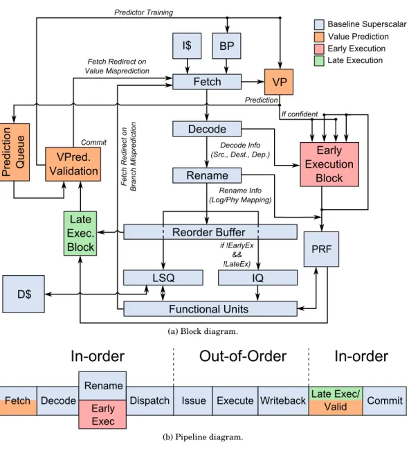
As previously described, EOLE consists of a set of simple ALUs in the in-order front-end to early-execute instructions in parallel with Rename, and a second set in the in-order back-end to late-execute instructions just before they are committed.
While EOLE is heavily dependent on Value Prediction, they are in fact complemen-tary features. Indeed, the former needs a value predictor to predict operands for Early Execution and provide temporal slack for Late Execution, while Value Prediction needs EOLE to reduce PRF complexity and thus become truly practical.
Moreover, to be implemented, EOLE requires prediction validation to be done at commit since validating at Execute mechanically forbids Late Execution. In addition, using selective replay to recover from a value misprediction nullifies the interest of both Early and Late Execution as all instructions must flow through the out-of-order scheduler in case they need to be replayed [Kim and Lipasti 2004]. Hence, squashing
(a) Block diagram.
(b) Pipeline diagram.
Fig. 1: The EOLE µ-architecture.
must be used to recover from a misprediction so that early/late executed instructions can safely bypass the scheduler.
Fortunately, [Perais and Seznec 2014b] have proposed a confidence estimation mech-anism greatly limiting the number of value mispredictions, Forward Probabilistic Counters (FPC). With FPC, the cost of a single misprediction can be high since mispre-dicting is very rare. Thus, validation can be done late – at commit time – and squashing can be used as the recovery mechanism. This enables the implementation of both Early and Late Execution, hence EOLE.
By eliminating the need to dispatch and execute many instructions in the out-of-order engine, EOLE substantially reduces the pressure put on complex and power-hungry structures. Thus, those structures may be scaled down, yielding a less complex
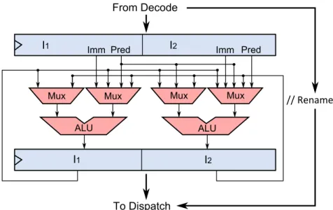
Fig. 2: Early Execution Block. The logic controlling the ALUs and muxes is not shown for clarity.
architecture whose performance is on par with a more aggressive design. Moreover, doing so is orthogonal to previously proposed mechanisms such as clustering [Farkas et al. 1997; Kessler et al. 1998; Palacharla et al. 1997; Seznec et al. ] and does not require a centralized instruction window, even though this is the model we use in this paper. Figure 1 depicts the EOLE architecture, implementing both Early Execution (red), Late Execution (green) and Value Prediction (orange). In the following para-graphs, we detail the two additional blocks required to implement EOLE and their interactions with the rest of the pipeline.
3.2. Early Execution Hardware
The core idea of Early Execution (EE) is to position one or more ALU stages in the front-end in which instructions with available operands will be executed. For com-plexity concerns, however, it seems necessary to limit Early Execution to single-cycle ALU instructions. Indeed, implementing complex functional units in the front-end to execute multi-cycle instructions does not appear as a worthy tradeoff. In particular, memory instructions are not early executed. EE is done in-order, hence, it does not require renamed registers and can take place in parallel with Rename. For instance, Figure 2 depicts the Early Execution Block adapted to a 2-wide Rename stage.
Renaming is often pipelined over several cycles. Consequently, we can use several ALU stages and simply insert pipeline registers between each stage. The actual exe-cution of an instruction can then happen in any of the ALU stages, depending on the readiness of its operands coming from Decode (i.e., immediate), the local4bypass
net-work (i.e., from instructions early executed in the previous cycle) or the value predictor. Operands are never read from the PRF.
4For complexity concerns, we consider that bypass does not span several ALU stages. Consequently, if an
instruction depends on a result computed by an instruction located two rename-groups ahead, it will not be early executed.
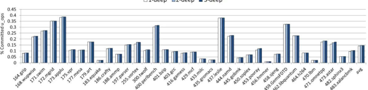
Fig. 3: Proportion of committed instructions that can be early executed, using one or two ALU stages and a D-VTAGE hybrid predictor (later described in Section 4).
In a nutshell, all eligible instructions flow through the ALU stages, propagating their results in each bypass network accordingly once they have executed. Finally, after the last stage, results as well as predictions are written into the PRF.
An interesting design concern lies with the number of stages required to capture a reasonable proportion of instructions. We actually found that using more than a single stage was highly inefficient, as illustrated in Figure 3. This Figure shows the proportion of committed instructions eligible for Early Execution for a baseline 8-wide rename, 6-issue model (see Table I in Section 4), using the D-VTAGE value predictor (later described in Table II, Section 4). As a result, in further experiments, we consider a 1-deep Early Execution Block only.
To summarize, Early Execution only requires a single new block, which is shown in red in Figure 1. The mechanism we propose does not require any storage area for temporaries as all values are living inside the pipeline registers or the bypass net-work(s). Finally, since we execute in-order, each instruction is mapped to a single ALU and scheduling is straightforward (as long as there are as many ALUs as the rename width).
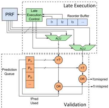
3.3. Late Execution Hardware
Late Execution (LE) targets instructions whose result has been predicted. Instructions eligible for prediction are µ-ops producing a 64-bit or less result that can be read by a subsequent µ-op, including non-architectural temporary registers, as defined by the ISA implementation. Unless mentioned otherwise, vector and scalar SIMD instruc-tions are not predicted.
Late Execution intervenes just before prediction validation time, that is, out of the execution engine. As for Early Execution, we limit ourselves to single-cycle ALU in-structions to minimize complexity. That is, predicted loads are executed in the out-of-order engine, but validated at commit.
Interestingly, [Seznec 2011] showed that conditional branch predictions flowing from TAGE can be categorized such that very high confidence predictions are known. Since high confidence branches exhibit a misprediction rate generally lower than 0.5%, re-solving them in the Late Execution block will have a marginal impact on overall perfor-mance. Thus, we consider both single-cycle predicted ALU instructions and very high confidence branches5for Late Execution. In this study, we did not try to set confidence
on the other branches (indirect jumps, returns). Yet, provided a similar high confidence estimator for these categories of branches, one could postpone the resolution of high confidence ones until the LE stage.
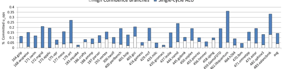
Fig. 4: Proportion of committed instructions that can be late executed using a D-VTAGE (see Section 4) hybrid predictor. Late executable instructions that can also be early executed are not counted since instructions are executed at most once.
Furthermore, note that predicted instructions can also be early executed. In that event, they only need to be validated in case another early executed instruction from the same rename-group used the prediction as an operand. That is, instructions are executed in a single location.
In any case, Late Execution further reduces pressure on the out-of-order engine in terms of instructions dispatched to the scheduler. As such, it also removes the need for value predicting only critical instructions [Fields et al. 2001; Rychlik et al. 1998; Tune et al. 2002] since minimizing the number of instructions flowing through the out-of-order engine requires maximizing the number of predicted instructions. Hence, pre-dictions considered as useless from a performance standpoint become useful in EOLE. Figure 4 shows the proportion of committed single-cycle ALU instructions that can be late executed using a baseline 6-issue processor with a D-VTAGE predictor (respec-tively described in Tables I and II in Section 4).
Late Execution needs to implement commit width ALUs and the associated read ports in the PRF. If an instruction I1 to be late executed depends on the result of
instruction I0 of the same commit group that will also be late executed, it does not
need to wait as it can use the predicted result of I0. In other words, all non executed
instructions reaching the Late Execution stage have all their operands ready in the PRF, as in DIVA [Austin 1999]. Due to the need to validate predictions (including reading results to train the value predictor) as well as late-execute some instructions, at least one extra pipeline stage after Writeback is likely to be required in EOLE. In the remainder of this paper, we refer to this stage as the Late Execution/Validation and Training (LE/VT) stage.
Overall, the hardware needed for LE is fairly simple, as suggested by the high-level view of a 2-wide LE Block shown in Figure 5. It does not even require a bypass network. In further experiments, we consider that LE and prediction validation can be done in the same cycle, before the Commit stage. EOLE is therefore only one cycle longer than the baseline superscalar it is compared to. While this may be optimistic due to the need to read from the PRF, this only impacts the value misprediction penalty, the pipeline fill delay, and ROB occupancy. In particular, since low confidence branches are resolved in the same cycle as for the baseline, the average branch misprediction penalty will remain very similar. Lastly, as a first step, we also consider that enough ALUs are implemented (i.e., as many as the commit-width). As a second step, we shall consider reduced-width Late Execution.
Fig. 5: Late Execution Block for a 2-wide processor. The top part can late-execute two instructions while the bottom part validates two results against their respective pre-dictions. Buses are general purpose register-width-bit wide.
3.4. Potential out-of-order Engine Offload
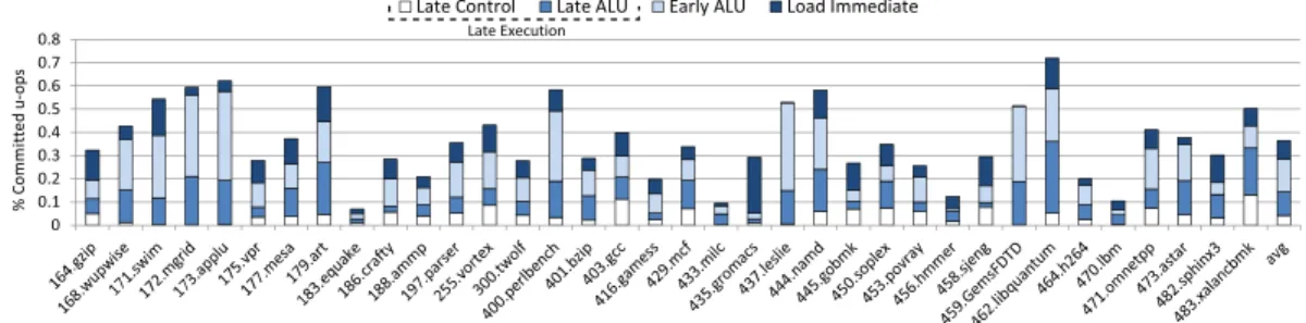
3.4.1. Baseline. We obtain the ratio of retired instructions that can be offloaded from the out-of-order engine for each benchmark by summing the columns in Figure 3 and 4 (both sets are disjoint as we only count late executable instructions that cannot also be early executed), and adding load immediate instructions. Those numbers are reported in Figure 6 where we distinguish four types of instructions:
(1) Early executed because it is a load immediate, i.e., its operand is necessarily ready at Rename.6 In a regular Value Prediction pipeline, these instructions can also
bypass the out-of-order engine as the immediate can be considered as an always correct value prediction. This includes loading an immediate to a floating point register.
(2) Early executed because it is a ready single-cycle ALU instruction.
(3) Late executed because it is a high-confidence branch, as predicted by the TAGE branch predictor.
(4) Late executed because it is a value predicted single-cycle ALU instruction.
We observe that the ratio is very dependent on the application, ranging from less than 10% for equake, milc and lbm to more than 50% for swim, mgrid, applu, perl-bench, leslie, GemsFDTD, xalancbmk and up to 60% for namd and 70% for libquan-tum. It generally represents a significant part of the retired instructions in most cases (around 35% on average).
Fig. 6: Proportion of dynamic instructions that can bypass the execution engine by being a high-confidence branch, a value predicted ALU instruction, an ALU instruction with its operands ready in the frontend or a load immediate instruction.
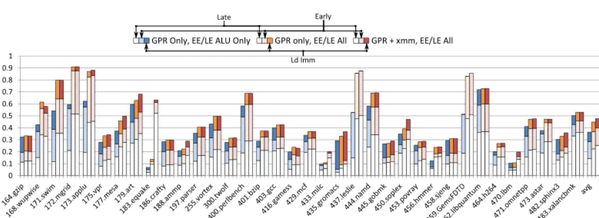
3.4.2. Limit Study.We also consider numbers when we do not specify any constraint regarding the type of instructions that can be early or late executed. In particular, all load and complex arithmetic (e.g., multiply, divide) instructions are considered for bypassing the execution engine. We also consider floating-point (FP) operations and packed vector operations (the shortcomings of actually predicting those types of in-structions are discussed in the next Section).
Figure 7 shows the overall potential either without FP/SIMD prediction (but still allowing loads and complex integer instructions to be early or late executed, second set of bars) and with FP/SIMD prediction (third set of bars). The first set of bars recalls the numbers of Figure 6.
The second set of bars (no FP/SIMD prediction, but all instructions are eligible for early/late execution) shows that in most case, allowing all instructions to be early/late executed significantly increases the proportion of instructions that can bypass the exe-cution engine. However, this increase is generally due to an increase in late-executable instructions (from 14.3% to 22.3% on average) rather than early-executable ones (from 14.1% to 14.5% on average). Moreover, in most cases, the bulk of the additional can-didates for late execution consists of value predicted loads. Indeed, on average, loads represent 26.2% of the predicted instructions versus 1.56% for other types of instruc-tions (multiplicainstruc-tions, divisions and conversions from float to int) that are now allowed to be early/late executed. As a result, allowing loads to be late executed would be of great help to further reduce pressure on the out-of-order engine.
The third set of bars (FP/SIMD prediction, all instructions are eligible for early/late execution) suggests that although the value predictor is able to predict a significant amount of instructions writing to xmm registers for a few benchmarks (e.g., equake, milc and soplex), the average increase in early/late-executable instructions is much lower than the one we observed by allowing loads and complex integer instructions to be early/late executed.
4. EVALUATION METHODOLOGY 4.1. Simulator
We use the x86 64 ISA to validate EOLE, even though EOLE can be adapted to any general-purpose ISA without any more restrictions than the ones already existing for Value Prediction. We use a modified7version of the gem5 cycle-level simulator [Binkert
et al. 2011].
7Our modifications mostly lie with the ISA implementation. In particular, we implemented branches with a
single µ-op instead of three and we removed some false dependencies existing between instructions due to the way flags are renamed/written.
Fig. 7: Proportion of dynamic instructions that can bypass the execution engine, de-pending on what kind of instructions are value predicted and what kind of instructions are allowed to be early/late executed.
We consider a relatively aggressive 4GHz, 6-wide issue superscalar8baseline with a
fetch-to-commit latency of 19 cycles. Since we focus on the out-of-order engine complex-ity, both in-order front-end and in-order back-end are overdimensioned to treat up to 8 µ-ops per cycle. We model a deep front-end (15 cycles) coupled to a shallow back-end (3 cycles) to obtain realistic branch/value misprediction penalties.
Table I describes the characteristics of the baseline pipeline we use in more details. In particular, the out-of-order engine is dimensioned with a unified centralized 60-entry scheduler (a.k.a. instruction queue or IQ) and a 192-60-entry Reorder Buffer (ROB) on par with Haswell’s, the latest commercially available Intel microarchitecture. We refer to this baseline as the Baseline 6 60 configuration (6-issue, 60-entry IQ). Func-tional units are grouped by stacks, to mimick the behavior of Haswell’s issue ports as best as possible. Note that there are 8 stacks, but since we consider a 6-issue processor, at most 6 stacks will be assigned an instruction each cycle.
In that context, reducing the issue width can be achieved in two fashions. First, by simply removing some issue ports. The associated FUs can then be redistributed to other ports, or be totally discarded from the design. Second, by keeping the same FU stacks, but by only allowing new issue width instructions to be issued per cycle. An actual implementation will likely do the former, however, since finding the optimal mix of FUs per issue port is beyond the scope of this paper, we keep the same FU stacks for all the different issue widths we consider in our experiments.
As µ-ops are known at Fetch in gem5, all the widths given in Table I are in µ-ops, even for the Fetch stage. Independent memory instructions (as predicted by the Store Sets predictor [Chrysos and Emer 1998]) are allowed to issue out-of-order. Entries in the scheduler are released upon issue, except for load instructions, which release their entry at Writeback.
In the case where Value Prediction is used, we add a pre-commit stage responsible for validation/training and Late Execution when relevant : the LE/VT stage. This ac-counts for an additional pipeline cycle (20 cycles) and an increased value misprediction penalty (21 cycles min.). Minimum branch misprediction latency remains unchanged except for mispredicted very high confidence branches when EOLE is used. Note that
8On our benchmark set and with our baseline simulator, an 8-issue machine achieves only marginal speedup
over this baseline. Hence we consider an issue width of 6 to ensure that reducing it will noticeably decrease performance.
8-wide Decode
8-wide Rename + 8-wide Early Execution
Execution
8-wide Dispatch to:
192-entry Reorder Buffer, 60-entry unified scheduler (IQ), 72-entry Load Queue, 48-entry Store Queue
4K-entry SSID/LFST Store Sets [Chrysos and Emer 1998] memory depen-dency predictor
256/256 INT/FP – 64/128-bit SIMD registers are allocated from the pool of 64-bit FP registers
Each cycle, issue one instruction to 6 ports out of the following 8:
Port0: ALU(1c) ⊗ Mul(3c) ⊗ Div(25c*) ⊗ FP Mul(5c) ⊗ FP Div(10c*) ⊗ 128-bit SIMD FP Mul(5c)Div(25c*)⊗ 128-bit SIMD INT Mul(3c)
Port1: ALU(1c)⊗ FP(3c) ⊗ 128-bit SIMD ALU (1c INT, 3c FP) Port2: Ld/Str Port3: Ld/Str Port4: ALU(1c) Port6: ALU(1c) Port7: Str 8-wide Writeback
8-wide Validation (only when VP is used) + 8-wide Late Execution 8-wide Commit
Caches
L1D 8-way 32KB, 4 cycles, 64 MSHRs, 2 reads and 2 writes/cycle, perfect D-TLB
Unified L2 16-way 1MB, 12 cycles, 64 MSHRs, no port constraints L2 Stride prefetcher, degree 8
All caches have 64B lines and LRU replacement
Memory Single channel DDR3-1600 (11-11-11), 2 ranks, 8 banks/rank, 8K row-buffer,tREFI 7.8us; Min. Read Lat.: 75 cycles, Max. 185 cycles.
the value predictor is really trained after Commit, but the value is read from the PRF in the LE/VT stage.
Shortcomings of the Model. Contrarily to modern x86 implementations, gem5 does not support move elimination [Fahs et al. 2005; Jourdan et al. 1998; Petric et al. 2005], µ-op fusion [Gochman et al. 2003] and does not implement a stack-engine [Gochman et al. 2003]. It also lacks macro-op fusion, zero-idioms elimination (e.g., xor rax, rax), as well as a µ-op cache [Intel 2014].
Although breaking true data dependencies through VP can overlap with some of these features (e.g., zero-idioms elimination and stack engine), most of them are or-thogonal, therefore, the inherent increase in ILP brought by VP should not generally be shadowed by said optimizations. In other words, the pipeline we model is sufficiently resembling a modern superscalar processor to illustrate how VP can push performance higher and how it can help reduce the aggressiveness of the execution engine.
ments.
In addition, we point out that correctly predicting a L1 hit would still potentially save 4 cycles in Haswell, but would more importantly allow more freedom regarding speculative scheduling [Kim and Lipasti 2004]. That is, since load dependents can use the prediction to execute, there is no need to schedule them speculatively assuming the load will hit and no bank conflict will take place in the L1 (if the L1 is banked). As a result, scheduling replays due to L1 misses and L1 bank conflicts (hit in L1 but the cache bank is busy) can be avoided if the aforementioned load is value-predicted.
4.2. Value Predictor Operation
The predictor makes a prediction at fetch time for every eligible µ-op (we define eligible in the next paragraph). To index the predictor, we XOR the PC of the x86 64 instruction with the µ-op number inside the x86 64 instruction. This avoids all µ-ops mapping to the same entry for x86 instructions generating more than one µ-op. We assume that the predictor can deliver as many predictions as requested by the Fetch stage.
In previous work, a prediction is written into the PRF and replaced by its non-speculative counterpart when it is computed in the out-of-order engine [Perais and Seznec 2014b]. In parallel, predictions are put in a FIFO queue to be able to validate them – in-order – at commit time. In EOLE, we also use a queue for validation. How-ever, instead of directly writing predictions to the PRF, we place predictions in the Early Execution units, which will in turn write the predictions to the PRF at Dispatch. By doing so, we can use predictions as operands in the EE units.
Eligible µ-ops. Since the predictor is able to produce 64-bit values, all µ-ops writing to a 64-bit (or less) General Purpose Register (GPR) are predicted, including instruc-tions that convert a floating-point value to an integer value (e.g., Convert Single Scalar FP to Signed D/Qword, CVTSS2SI).
In addition, gem5-x86 splits 128-bit packed instructions into two 64-bit (32-bit packed or 64-bit scalar) µ-ops.9As a result, it appears possible to predict floating-point
results (both scalar and vector), as well as packed integer results, and in our first ex-periments, we consider doing so. However, cracking packed instructions into several µ-ops is not representative of a high-performance implementation. Thus, predicting packed 128-bit (or more) registers would in fact involve looking-up several predictor entries for the same µ-op, or provision 128 bits (or more) in each predictor entry, which may not be practical. Consequently, our final experiments do not consider packed in-structions as a target for value prediction.
Nonetheless, scalar floating-point operations produce a 64-bit (or 32-bit for single-precision FP) value, therefore, it should be possible to predict them. Unfortunately, both encodings (legacy and VEX since AVX) of the x86 FPU, SSE, require that a scalar operation on a SIMD register copies the upper part of the first source xmm register to
9Both can be executed in a single cycle in our model, hence execution throughput is still 128 bits per cycle
VEX-encoded:
dest[63:0] = src1[63:0] + src2[63:0] dest[127:64] = src1[127:64]
dest[255:128] = 0
Consequently, although the functional unit computes a 64-bit value, the need to merge the physical destination register with one physical source register yields an effective result width of 256 bits (Legacy) and 128 bits (VEX-encoded). Hence, except for scalar loads (which zero the upper part of both xmm and ymm), it is not useful to predict scalar floating point results,12because the RAW dependency is not broken by
the prediction.
Note however that this limitation is purely inherent to the ISA, and that it would be possible to overcome it at the microarchitectural level, for instance by allowing differ-ent parts of a single ymm/xmm register to be renamed to differdiffer-ent physical registers, and injecting a merge µ-op where appropriate.13 Since this would allow to eliminate
many copies of the upper part of xmm registers, this might in fact be an optimization that is already implemented. In that event, predicting scalar FP instructions would be possible.
To summarize, while we consider predicting all results (i.e., scalar/vector integer and scalar/vector floating-point) as a first step, to gauge the potential for additional performance and the predictability of FP results, we will ultimately consider predicting values that are written to a general purpose register only, as predicting scalar FP operations requires microarchitectural support due to ISA limitations, and FP load coverage tends to be very low, on our benchmark set.
x86 Flags. In the x86 64 ISA, some instructions write flags based on their results while some need them to execute (e.g., conditional branches) [Intel 2013]. We assume that flags are computed as the last step of Value Prediction, based on the predicted value. In particular, the Zero Flag (ZF), Sign Flag (SF) and Parity Flag (PF) can easily be inferred from the predicted result. Remaining flags – Carry Flag (CF), Adjust Flag (AF) and Overflow Flag (OF) – depend on the operands and cannot be inferred from the predicted result only. We found that always setting the Overflow Flag to 0 did not cause many mispredictions and that setting CF if SF was set was a reasonable approx-imation. The Adjust Flag, however, cannot be set to 0 or 1 in the general case. This is a major impediment to the value predictor coverage since we consider a prediction as incorrect if one of the derived flags – thus the flag register – is wrong. Fortunately, x86 64 forbids the use of decimal arithmetic instructions. As such, AF is not used and we can simply ignore its correctness when checking for a misprediction [Intel 2013].
10In the legacy encoding, the first source is also the destination register, but the copy of the upper part of
the old physical register to the new one is still required.
11128-bit xmm registers correspond to the lower 128 bits of 256-bit ymm registers.
12At least for SSE/AVX, which is the current FPU ISA for x86, x87 being deprecated [Intel 2013]. 13This is also a way to handle x86 general purpose partial registers.
Predictor Considered in this Study. In this study, we focus on the tightly-coupled hybrid of VTAGE and a simple stride-based Stride predictor, D-VTAGE [Perais and Seznec 2015]. For confidence estimation, we use Forward Probabilistic Counters [Perais and Seznec 2014b]. In particular, we use 3-bit confidence counters whose for-ward transitions are controlled by the vector v = {1, 1
16, 1 16, 1 16, 1 16, 1 32, 1 32} as we found it
to perform best with D-VTAGE. Those counters allow to push accuracy very high while only requiring 3-bit per counter (The Linear Feedback Shift Register used to provide randomness is amortized on the whole predictor, or a large number of entries). This is required to absorb the cost of validating predictions at Commit and squashing to recover.
We consider an 8K-entry base predictor and 6 1K-entry partially tagged components. We do not try to optimize the size of the predictor (by using partial strides, for in-stance), but it has been shown that 16 to 32KB of storage are sufficient to get good performance with D-VTAGE [Perais and Seznec 2015].
4.3. Benchmarks
We use a subset of the the SPEC’00 [Standard Performance Evaluation Corporation 2000] and SPEC’06 [Standard Performance Evaluation Corporation 2006] suites to evaluate our contribution as we focus on single-thread performance. Specifically, we use 18 integer benchmarks and 18 floating-point programs.14 Table III summarizes
the benchmarks we use as well as their input, which are part of the reference inputs provided in the SPEC software packages. To get relevant numbers, we identify a region of interest in the benchmark using Simpoint 3.2 [Perelman et al. 2003]. We simulate the resulting slice in two steps: First, warm up all structures (caches, branch predictor and value predictor) for 50M instructions, then collect statistics for 100M instructions. Note that the baseline simulator configuration we use in this work is significantly different from the configuration used in [Perais and Seznec 2014a]: Fetch is less ag-gressive, the last level cache is smaller, the first level data cache is slower, and much less complex functional units and loads ports are implemented. Thus, a more realistic pipeline configuration is simulated, but the IPC in some benchmarks is much lower (e.g., vpr has 0.664 vs. 1.326 and art has 0.441 vs. 1.211). On the contrary, since we use a bigger LQ (72-entry vs 48-entry in [Perais and Seznec 2014a]) to better fit the Intel Haswell pipeline configuration, and since we use a bigger and better implementation of the Store Sets memory dependency predictor, IPC is higher in other benchmarks (e.g., gamess has 2.196 vs. 1.929 and parser has 0.872 vs. 0.544). In almost all cases, the gains come from the better memory dependency predictor, and we actually found that in the version of gem5 used in [Perais and Seznec 2014a], the PC of memory instruc-tions is right-shifted by 2 before accessing the table, accommodating 4-byte aligned RISC but not x86’s CISC.
171.swim (FP) swim.in 2.206
172.mgrid (FP) mgrid.in 2.356
173.applu (FP) applu.in 1.481
175.vpr (INT)
net.in arch.in place.out dum.out -nodisp place only init t 5 exit t 0.005 -alpha t 0.9412 -inner num 2
0.664
177.mesa (FP) -frames 1000 -meshfile mesa.in -ppmfilemesa.ppm 1.268
179.art (FP)
scanfile c756hel.in trainfile1 a10.img trainfile2 hc.img stride 2 startx 110 -starty 200 -endx 160 -endy 240 -objects 10
0.441
183.equake (FP) inp.in 0.655
186.crafty (INT) crafty.in 1.551
188.ammp (FP) ammp.in 1.212
197.parser (INT) ref.in 2.1.dict -batch 0.872
255.vortex (INT) lendian1.raw 1.795
300.twolf (INT) ref 0.468
400.perlbench (INT) -I./lib checkspam.pl 2500 5 25 11 150 1
1 1 1 1.370
401.bzip2 (INT) input.source 280 0.780
403.gcc (INT) 166.i 1.028
416.gamess (FP) cytosine.2.config 2.196
429.mcf (INT) inp.in 0.116
433.milc (FP) su3imp.in 0.499
435.gromacs (FP) -silent -deffnm gromacs -nice 0 0.792
437.leslie3d (FP) leslie3d.in 2.139 444.namd (FP) namd.input 2.347 445.gobmk (INT) 13x13.tst 0.845 450.soplex (FP) -s1 -e -m45000 pds-50.mps 0.271 453.povray (FP) SPEC-benchmark-ref.ini 1.519 456.hmmer (INT) nph3.hmm 2.016
458.sjeng (INT) ref.txt 1.302
459.GemsFDTD (FP) / 2.146
462.libquantum (INT) 1397 8 0.460
464.h264ref (INT) foreman ref encoder baseline.cfg 1.127
470.lbm (FP) reference.dat 0.373
471.omnetpp (INT) omnetpp.ini 0.309
473.astar (INT) BigLakes2048.cfg 1.166
482.sphinx3 (FP) ctlfile . args.an4 0.787 483.xalancbmk (INT) -v t5.xml xalanc.xsl 1.934
Fig. 8: Speedup over Baseline 6 60 brought by Value Prediction using D-VTAGE. In-structions eligible for VP are either those writing a GPR register (GPR), or all instruc-tions writing a register (GPR + xmm).
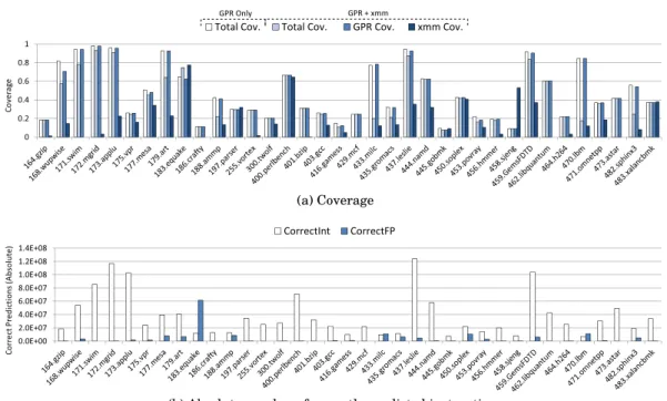
(a) Coverage
(b) Absolute number of correctly predicted instructions
Fig. 9: Relative and absolute coverage of the D-VTAGE predictor.
5. EXPERIMENTAL RESULTS
In our experiments, we first use Baseline 6 60 as the baseline to gauge the impact of adding a value predictor only. Then, in all subsequent experiments, we use Base-line 6 60 augmented with the predictor presented in Table II as our performance base-line. We refer to it as the Baseline VP 6 60 configuration. Our objective is to charac-terize the potential of EOLE at decreasing the complexity of the out-of-order engine. We assume that the Early and Late Execution stages are able to treat any group of up to 8 consecutive µ-ops every cycle. In Section 6, we will consider tradeoffs to enable realistic implementations.
structions writing to 128-bit xmm registers, including integer and FP vector instruc-tions. As previously mentioned, gem5-x86 splits a 128-bit instruction into two 64-bit ones, therefore, from the point of view of the predictor, a single packed instruction is in fact two scalar (or 64-bit packed) µ-ops. In general, performance is comparable to the previous case, yet, in applu, mesa, art, equake, namd, soplex and h264, a slight performance increase can be observed, while a slight decrease can be seen in wupwise, gamess and leslie.
To gain some insight on why we observe such behavior, we consider the overall cov-erage of the value predictor, as well as the covcov-erage for integer and FP instructions in Figure 9 (a). The first observation is that in general, FP coverage15is much lower
than integer coverage. This is expected since a stride-based prediction scheme cannot naturally predict FP values other than constants. In some cases, however, FP coverage is higher (e.g., equake, gobmk, sjeng and xalancbmk). Yet, since coverage is a relative metric, it is not representative of how many instructions are actually predicted. As a result, Figure 9 (b) shows the absolute number of predicted instructions. Except in one benchmark (equake), the number of predicted FP instructions is often quite low, and in particular, lower than the number of integer predictions. As a result, in two out of the four previously mentioned cases where FP coverage is higher than INT coverage (sjeng and xalancbmk), the absolute number of predicted FP instructions is actually very low.
Regardless, benchmarks where performance increases slightly have a similar level of integer coverage as in the “integer prediction only” case, but they are also able to predict a small (applu, art, h264, namd) to moderate (mesa, equake, soplex) amount of FP instructions. On the contrary, when performance decreases, integer coverage is lower than in the “integer prediction only” case, and the small FP coverage does not make up for this reduction. This phenomenon can be explained by the fact that more static instructions have to share the PC-indexed Last Value Table (LVT) of D-VTAGE, hence potential decreases because more instructions collide in the LVT.
Nonetheless, it is interesting to note that in equake, many FP instructions are ac-tually predictable (the majority being scalar single-precision additions and multiplica-tions, but not loads from memory), hinting that although stride-based prediction does not match the floating-point representation, there are still some FP computations that show enough redundancies to benefit from having a value predictor.
5.2. Issue Width Impact on Processor Performance
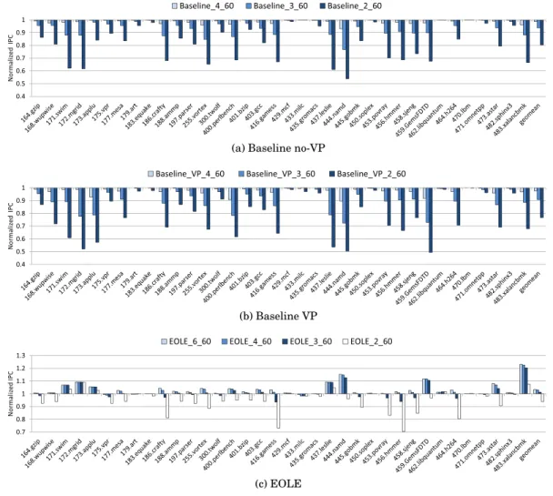
Baseline VP Model. We first depict the performance loss implied by reducing the issue-width on the baseline processor, Baseline 6 60, in Figure 10 (a). As the issue width is reduced, performance often decreases, but Baseline 4 60 generally performs within 5% of Baseline 6 60, with a maximum slowdown of 7% in namd.
We also experimented with VP (Baseline VP 6/4/3/2 60) in Figure 10 (b). It is quite clear that although the average performance of the 4-issue pipeline is close to
(a) Baseline no-VP
(b) Baseline VP
(c) EOLE
Fig. 10: Impact of a reduced issue width on performance, normalized to Baseline 6 60 in (a) and Baseline VP 6 60 in (b,c).
that of the 6-issue one, up to 10% performance is lost in applu, perlbench, namd and GemsFDTD. Moreover, reducing the issue width beyond 4 is clearly detrimental, as average performance is 90% that of the 6-issue pipeline for a 3-issue processor, and less than 80% for a 2-issue processor (with a maximum slowdown of 50% in namd and GemsFDTD).
As a result, the reduction in execution engine complexity comes at a noticeable cost in performance when VP is implemented. Without VP, less ILP can be extracted by the processor, and diminishing the issue width is less detrimental, although some bench-marks are still affected as soon as the issue width is decreased to 4.
EOLE. The performance of EOLE is illustrated in Figure 10 (c), using different out-of-order issue widths.
On top of the 6-issue VP pipeline, EOLE slightly increases performance over the baseline, with a few benchmarks achieving 5% speedup or higher (first bar). The par-ticular case of namd is worth to be noted as with VP only, it would have benefited from an 8-issue core by more than 10%. Through EOLE, we actually increase the number of
performance, with slowdowns of around 5% being observed in gamess, povray, hmmer and h264 on the 3-issue pipeline. As a result, EOLE can be considered as a means to reduce issue width without significantly impacting performance on a processor featur-ing VP, as long as the execution engine remains wide enough (e.g., 4-issue).
5.3. Impact of Instruction Queue Size on Processor Performance
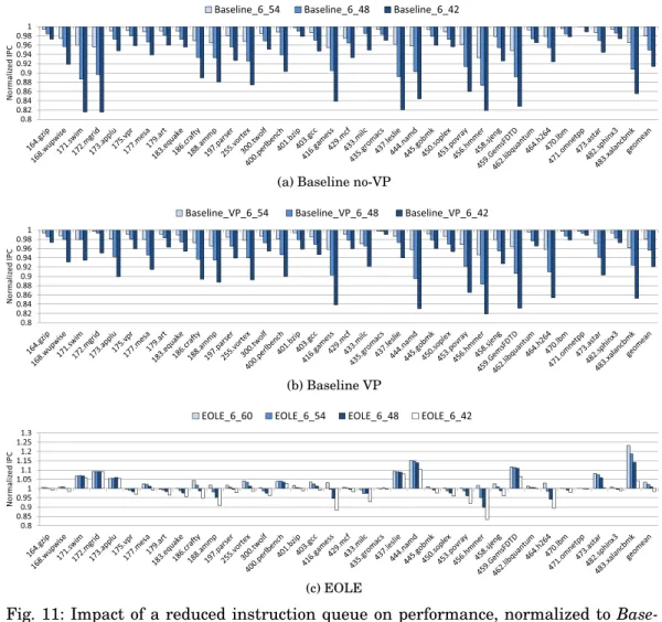
Baseline VP Model. In Figure 11 (a), we illustrate the performance loss inherent to the reduction in the number of instruction queue entries for the baseline model. Since VP is not present, ILP is often lower, hence instructions stay longer in the scheduler. This leads to performance decreasing noticeably even when only 6 IQ entries are re-moved (e.g., gamess, leslie, namd, hmmer and GemsFDTD), which is not desirable.
Figure 11 (b) shows results for the baseline VP pipeline. Since ILP is higher, instruc-tions stay less longer in the IQ, and the performance drop is generally less significant than without VP. However, although the maximum slowdown is less than when the issue width is reduced, almost all benchmarks are slowed down even when only six entries are removed (first bar). On average (gmean), 2% performance is lost, with a maximum of 5.4% in hmmer. Further reducing the instruction queue size has even more detrimental effects, with an average performance loss of 4% and 8% for a 48-entry and a 42-48-entry IQ, respectively.
EOLE. With EOLE, the performance loss is much less pronounced in general, as shown in Figure 11 (c). Yet, even when only six entries are removed from the IQ, a 5% performance degradation is observed in hmmer, which is still problematic as our goal is to keep at least the same level of performance as the baseline VP model.
In practice, the benefit of EOLE is greatly influenced by the proportion of instruc-tions that are not sent to the out-of-order engine. For instance namd needs a 60-entry IQ in the baseline case, but since it is an application for which many instructions are early or late executed, it can deal with a smaller IQ in EOLE.
On the other hand, hmmer, the application that suffers the most from reducing the instruction queue size with EOLE, exhibits a relatively low coverage of predicted or early executed instructions.
5.4. Summary
EOLE provides opportunities for either slightly improving the performance over a VP-augmented processor without increasing the complexity of the execution engine, or reaching the same level of performance with a significantly reduced execution engine complexity. Said complexity can be reduced via two means: reducing the issue width, and reducing the IQ size.
Reducing the issue width reduces the number of broadcast buses used for Wakeup as well as the complexity of the Select operation. Moreover, the maximum number of ports required on the PRF is reduced, and finally, the number of values co-existing in the bypass network each cycle is also reduced.
Reducing the number of IQ entries, on the contrary, does not reduce the number of broadcast buses, PRF ports and inflight values inside the bypass network. It only
(a) Baseline no-VP
(b) Baseline VP
(c) EOLE
Fig. 11: Impact of a reduced instruction queue on performance, normalized to Base-line 6 60 in (a) and BaseBase-line VP 6 60 in (b,c).
reduces the delay and the power spent in Wakeup by having shorter broadcast buses, as well as the Select delay since less entries have to be scanned [Palacharla et al. 1997]. Regardless, EOLE does not appear as efficient at mitigating the performance loss inherent to a smaller IQ, hence reducing the issue width appears as the better choice overall.
In the next section, we provide directions to limit the global hardware complexity and power consumption induced by the EOLE design and the overall integration of VP in a superscalar processor.
6. HARDWARE COMPLEXITY
In the previous section, we have shown that, provided that the processor already imple-ments Value Prediction, adopting the EOLE design may allow to use a reduced-issue execution engine without impairing performance. Yet, extra complexity and power con-sumption are added in the Early Execution engine as well as the Late Execution en-gine.
order issue width can be reduced from 6 to 4 without significant performance loss, on our benchmark set. This would greatly impact Wakeup since the complexity of each IQ entry would be lower. Similarly, a narrower issue width mechanically simplifies Select. As such, both steps of the Wakeup & Select critical loop could be made faster and/or less power hungry.
Providing a way to reduce complexity with no impact on performance is also cru-cial because modern schedulers must support complex features such as speculative scheduling and thus selective replay to recover from scheduling mispredictions [Kim and Lipasti 2004; Perais et al. 2015].
Lastly, to our knowledge, most scheduler optimizations proposed in the literature can be added on top of EOLE. This includes the Sequential Wakeup of [Kim and Li-pasti 2003] or the Tag Elimination of [Ernst and Austin 2002]. As a result, power consumption and cycle time could be further decreased.
Functional Units & Bypass Network. As the number of cycles required to read a register from the PRF increases, the bypass network becomes more crucial. It allows an instruction to “catch” its operands as they are produced and thus execute back-to-back with its producer(s). However, a full bypass network is very expensive, especially as the issue width – hence the number of functional units – increases. [Ahuja et al. 1995] showed that partial bypassing could greatly impede performance, even for a simple in-order single-issue pipeline. Consequently, in the context of a wide-issue out-of-order superscalar with a multi-cycle register read, missing bypass paths may cripple performance even more.
EOLE allows to reduce the issue width in the out-of-order engine. Therefore, it re-duces the design complexity of a full bypass by reducing the number of simultaneous writers on the network.
A Limited Number of Register File Ports on the out-of-order Engine. Through reduc-ing the issue width on the out-of-order engine, EOLE mechanically reduces the max-imum number of read and write ports required on the PRF for regular out-of-order execution.
6.2. Extra Hardware Complexity Associated with Late/Early Execution
Cost of the Late Execution Block. The extra hardware complexity associated with Late Execution consists of three main components. First, for validation at commit time, a prediction queue (FIFO) is required to store predicted results. This compo-nent is needed anyway as soon as VP associated with validation at commit time is implemented, since the prediction must be stored until it can be compared against the actual result at Commit.
Second, ALUs are needed for Late Execution. Lastly, the operands for the late ex-ecuted instructions must be read from the PRF. Similarly, the result of VP-eligible instructions must be read from the PRF for validation (predicted instructions only) and predictor training (all VP-eligible instructions).
In the simulations presented in Section 5, we have assumed that up to 8 µ-ops (i.e. commit-width) could be late executed per cycle. This would necessitate 8 ALUs
a full 8-to-8 bypass network and 8 write ports on the PRF.
The Physical Register File. From the above analysis, an EOLE-enhanced core featur-ing a 4-issue out-of-order engine (EOLE 4 60) would have to implement a PRF with a total of 12 write ports (resp. 8 for Early Execution and 4 for regular execution) and 24 read ports (resp. 8 for regular execution and 16 for late execution, validation and training).
The area cost of a register file is approximately proportional to (R + W ) ∗ (R + 2W ), R and W respectively being the number of read and write ports [Zyuban and Kogge 1998]. That is, at equal number of registers, the area cost of the EOLE PRF would be 4 times the initial area cost of the 6-issue baseline without value prediction (Base-line 6 60) PRF. Moreover, this would also translate in largely increased power con-sumption and access time, thus impairing cycle time and/or lengthening the register file access pipeline.
Without any optimization, Baseline VP 6 60 would necessitate 14 write ports (resp. 8 to write predictions and 6 for the out-of-order engine) and 20 read ports (resp. 8 for validation/training and 12 for the out-of-order engine), i.e., slightly less than EOLE 4 60. In both cases, this overhead might be considered as prohibitive in terms of silicon area, power consumption and access time.
Fortunately, simple solutions can be devised to reduce the overall cost of the PRF and the global hardware cost of Early/Late Execution without significantly impacting global performance. These solutions apply for EOLE as well as for a baseline imple-mentation of VP. We describe said solutions below.
6.3. Mitigating the Hardware Cost of Early/Late Execution
6.3.1. Mitigating the Early-Execution Hardware Cost.Because Early Executed instructions are processed in-order and are therefore consecutive, one can use a banked PRF and force the allocation of physical registers for the same dispatch group to different reg-ister banks. For instance, considering a 4-bank PRF, out of a group of 8 consecutive µ-ops, 2 could be allocated to each bank. In this fashion, a dispatch group of 8 consecu-tive µ-ops would at most write 2 registers in a single bank after Early Execution. Thus, Early Execution would necessitate only two extra write ports on each PRF bank, as il-lustrated in Figure 12 for an 8-wide Rename/Early Execute, 4-issue out-of-order core. Interestingly, this would add-up to the number of write ports required by a baseline 6-issue out-of-order core.
In Figure 13, we illustrate simulation results with a banked PRF. In particular, registers from distinct banks are allocated to consecutive µ-ops and Rename is stalled if the current bank does not have any free register. We consider respectively 2 banks of 128 registers, 4 banks of 64 registers and 8 banks of 32 registers. We observe that the performance loss associated with load unbalancing is quite limited for our benchmark set for the 2- and 4-bank configuration. Therefore, using 4 banks of 64 registers instead of a single bank of 256 registers appears as a reasonable tradeoff. However, using 8 banks of 32 registers begins to impact performance as Rename has to stall more often because there are no free registers in a given bank.
Fig. 12: Organization of a 4-bank PRF supporting 8-wide Early Execution/prediction and 4-wide out-of-order issue. Read ports dedicated to prediction validation and Late Execution are not shown.
Fig. 13: Performance of EOLE 4 60 using a different number of banks in the PRF, normalized to EOLE 4 60 with a single bank.
Note that register file banking is also a solution for a practical implementation of a core featuring Value Prediction without EOLE, since validation is also done in-order. Therefore, only two read ports are necessary (assuming 4 banks) to validate 8 µ-ops per cycle.
6.3.2. Limited Late Execution and Port Sharing. Not all instructions are predicted or late-executable (i.e., predicted and simple ALU or high confidence branches). Moreover, entire groups of 8 µ-ops are rarely ready to commit. Therefore, one can limit the num-ber of potentially late executed instructions and/or predicted instructions per cycle. For instance, the maximum commit-width can be kept to 8 with the extra constraint of using only 6 or 8 PRF read ports for Late Execution and Validation/Training.
Moreover, one can also leverage the register file banking proposed above to limit the number of read ports on each individual register file bank at Late Execution/Validation and Training. To only validate the prediction for 8 µ-ops and train the predictor, and assuming a 4-bank PRF, 2 read ports per bank would be sufficient. However, not all instructions need validation/training (e.g., branches and stores). Hence, some read ports may be available for LE, although extra read ports might be necessary to en-sure smooth LE.
Our experiments showed that limiting the number of read ports on each register file bank dedicated to LE/VT to only 4 results in a marginal performance loss. Figure 14 illustrates the performance of EOLE 4 60 with a 4-bank PRF and respectively 2, 3 and 4 ports provisioned for the LE/VT stage (per bank). As expected, having only two
ad-Fig. 14: Performance of EOLE 4 60 (4-bank PRF) when the number of read ports ded-icated to LE/VT is limited, normalized to EOLE 4 60 (1-bank PRF) with enough ports for full width LE/VT.
ditional read ports per bank is not sufficient. Having 4 additional read ports per bank, however, yields an IPC very similar to that of EOLE 4 60. Interestingly, adding 4 read ports adds up to a total of 12 read ports per bank (8 for out-of-order execution and 4 for LE/VT), that is, the same amount of read ports as the baseline 6-issue configuration. Note that provisioning only 3 read ports per bank is also a possibility as performance is also very close to the ideal EOLE 4 60.
It should be emphasized that the logic needed to select the group of µ-ops to be Late Executed/Validated on each cycle does not not require complex control and is not on the critical path of the processor. This could be implemented either by an extra pipeline cycle or speculatively after Dispatch.
6.3.3. The Overall Complexity of the Register File. Interestingly, on EOLE 4 60, the register file banking proposed above leads to equivalent performance as a non-constrained register file. However, the 4-bank file has only 2 extra write ports per bank for Early Execution and prediction and 4 extra read ports for Late Execu-tion/Validation/Training. That is a total of 12 read ports (8 for the out-of-order en-gine and 4 for LE/VT) and 6 write ports (4 for the out-of-order enen-gine and 2 for EE/Prediction), just as the baseline 6-issue configuration without VP.
As a result, if the additional complexity induced on the PRF by VP is noticeable (as issue width must remain 6), EOLE allows to virtually nullify this complexity by diminishing the number of ports required by the out-of-order engine. The only remain-ing difficulty comes from bankremain-ing the PRF. Nonetheless, accordremain-ing to the previously mentioned area cost formula [Zyuban and Kogge 1998], the total area and power con-sumption of the PRF of a 4-issue EOLE core is similar to that of a baseline 6-issue core without Value Prediction. Yet, performance is substantially higher since VP is present, as summarized in Figure 15.
It should also be mentioned that the EOLE structure naturally leads to a distributed register file organization with one file servicing reads from the out-of-order engine and the other servicing reads from the LE/VT stage. The PRF could be naturally built with a 4-bank, 6 write/8 read ports file (or two copies of a 6 write/4 read ports) and a 4-bank, 6 write/4 read ports one. As a result, the register file in the out-of-order engine would be less likely to become a temperature hotspot than in a conventional design.
6.3.4. Limiting the width of Early and Late Execution.So far, we have considered that re-name width and commit width ALUs were implemented in the Early Execution stage and the Late Execution stage, respectively. However, for the same reason that the num-ber of read ports dedicated to Late Execution can be limited, the width of EE and LE can be reduced. Indeed, since many instructions are not predictable or early/late
exe-Fig. 15: Performance of Baseline VP 6 60, EOLE 4 60 with 16 ports for LE/VT and a single bank and EOLE 4 60 using 4 ports for LE/VT and having 4 64-register banks, normalized to Baseline 6 60.
cutable, good enough performance can be attained with only a few additional simple ALUs overall.
Reducing the width of EE is especially interesting since EE requires a full bypass network to perform best. For instance, reducing the number of ALUs from 8 to 4 re-duces the bypass paths from 8-to-8 to 4-to-4. There is a caveat, however, in the fact that predicted results of instructions that are not early executed should also be made available to the next rename group. As a result, bypass is rather 8-to-4 than 4-to-4, since there still might be 8 results available for an 8-wide frontend.
Regardless, reducing the width of EE will not cause the pipeline to stall if too many instructions are eligible for Early Execution. Indeed, those instructions will simply have to be executed in the out-of-order engine (unless they are value predicted). On the contrary, reducing the width of Late Execution may stall the pipeline by limiting the number of instructions that can be committed, causing the ROB to become full. For instance, if eight instructions are late-executable but only two ALUs are present, then it will take four cycles to commit them, while the Commit stage could have retired them in a single cycle if 8 ALUs had been present.
Note that since we perform prediction validation at Late Execution, we consider that each LE ALU has the comparator required to do so. As a result, by reducing the number of LE ALUs, we also reduce the number of instructions whose prediction can be validated in order to train the predictor and squash on a misprediction. The maximum commit width of 8 remains attainable if the commit group contains enough instructions that do not produce a register (e.g., low confidence branches that were executed out-of-order, stores, etc.).
Figure 16 depicts the performance impact of decreasing the width of Early/Late Ex-ecution. The Figure shows IPC normalized to EOLE 4 60 with a 4-bank PRF and 4 read ports dedicated to LE/VT per PRF bank, and having 8-wide EE/LE stages. The first observation is that for an 8-wide Rename and an 8-wide Commit, 6-wide EE/LE is sufficient, as performance is comparable to having 8-wide EE/LE, except in namd (13.3% performance loss). Note however that performance in namd is still higher than the baseline 6-issue without VP (17.5% speedup).
However, as the EE/LE widths are decreased, performance degrades significantly, to attain 70% of the baseline when EE and LE are only 2-wide. Interestingly, using a 2-wide EE stage but a 6-wide LE stage has similar impact as using 6-wide EE/LE stages. This suggests that most of the performance loss is caused by the reduced-width LE stage, since it often limits the actual commit width, while the reduced-width EE stage only increases pressure on the execution engine. Consequently, while decreasing the EE width from 8 to only 2 does not impact performance significantly, keeping the
Fig. 16: Performance impact of reducing the width of Early/Late Execution. Normal-ized to EOLE 4 60 with a 4-bank PRF and 4 read ports dedicated to LE/VT, per PRF bank, and having 8-wide EE/LE stages.
LE width close to the commit width is necessary to limit pipeline stalls due to the ROB becoming full.
Furthermore, as mentioned in 3.4.2, a significant amount of value predicted instruc-tions are loads, which require validation but not late execution. Therefore, it is possible that the LE width could be decreased further if LE and prediction validation/training were to be implemented as two separate pipeline stages, and the validation/training width kept similar to the commit width.
6.4. Late Executing Predicted Loads
Most processors do not allow more than two loads to issue in the same cycle. The main reason is that adding ports to the data cache to handle more accesses is very expensive. Consequently, banking the data cache is generally preferred, but arbitration increases access latency and the number of bank conflicts will necessary increase with the num-ber of loads issued each cycle. As a result, it is not desirable to add a datapath between the data cache and the Late Execution stage as long as the execution engine already has the ability to issue two loads per cycle.
Nonetheless, by only allowing one load per cycle to be issued by the execution engine, we can move the second load port to the Late Execution stage. If the performance level of the baseline processor can be maintained, doing so may enable further reduction of the out-of-order engine aggressiveness.
Specifically, the Load Queue (LQ) is implemented to provide correctness in the pres-ence of out-of-order execution of memory operations. It can also be snooped by remote writes to enforce the memory model in some processors (e.g., x86 64 [Intel 2007]). Since late executed loads are executed in-order, they will not alias with an older store whose address is unknown, since all older stores have executed, by construction. As a result, it may not be necessary to add late executed loads to the LQ, depending on the memory model implemented by the processor.
6.4.1. Late Executing Loads.As a first step, and since we focus on single-core, we can ig-nore the fact that x86 64 is strongly ordered and consider that loads can safely bypass the LQ while allowing late-execution not to wait for older loads to return before mov-ing on to younger instructions.16 This essentially gives us the best of both world, by
potentially allowing to reduce the LQ size, while avoiding to stall the pipeline because the ROB became full waiting for a late executed load to complete while subsequent instructions could have been late executed in the meantime.