Lossless Image Compression via Predictive Coding of Discrete Radon Projections

HAL Id: hal-00287982

https://hal.archives-ouvertes.fr/hal-00287982

HAL is a multi-disciplinary open access

archive for the deposit and dissemination of sci-entific research documents, whether they are pub-lished or not. The documents may come from

L’archive ouverte pluridisciplinaire HAL, est destinée au dépôt et à la diffusion de documents scientifiques de niveau recherche, publiés ou non, émanant des établissements d’enseignement et de

Lossless Image Compression via Predictive Coding of

Discrete Radon Projections

Andrew Kingston, Florent Autrusseau

To cite this version:

Andrew Kingston, Florent Autrusseau. Lossless Image Compression via Predictive Coding of Discrete Radon Projections. Signal Processing: Image Communication, Elsevier, 2008, 23 (4), pp.313-324. �10.1016/j.image.2008.03.001�. �hal-00287982�

Lossless Image Compression via Predictive

Coding of Discrete Radon Projections

Andrew Kingston †‡, Florent Autrusseau †

† IRCCyN lab. Polytech’Nantes, Rue Ch. Pauc, BP 50609, 44306 Nantes, France ‡ Department of Applied Mathematics, Research School of Physical Sciences and

Engineering, Australian National University,Canberra, ACT 0200, Australia

Abstract

This paper investigates predictive coding methods to compress images represented in the Radon domain as a set of projections. Both the correlation within and between discrete Radon projections at similar angles can be exploited to achieve lossless compression. The discrete Radon projections investigated here are those used to define the Mojette Transform first presented by Gu´edon et al in 1995 [1]. This work is further to the preliminary investigation presented by Autrusseau et al in [2]. The 1D Mojette projections are re-arranged as two dimensions images, thus allowing the use of 2D image compression techniques onto the projections. Besides the compression capabilities, the Mojette transforms brings an interesting property: a tunable redundancy. As the Mojette transform is able to both compress and add redundancy, the proposed method can be viewed as a joint lossless source-channel coding technique for images. We present here the evolution of the compression ratio depending on the chosen redundancy.

1 Introduction

This work is motivated by the limitations of image processing tools in large multimedia databases. Numerous paintings belonging to French museums are stored in an image database within the “Centre of Research and

Restora-tion of French Museums” (C2RMF)1_{. It is required that these high payload}

(up to 1000 Megapixel) images be losslessly compressed, stored securely, (i.e., with some redundancy) and encrypted for transmission purposes. The French

TSAR project (Secure Transfer of High Resolution Art Images2_{) aims to}

de-velop a method to securely transfer images from the image database of artwork contained in the Louvre Museum. All this can also be said of medical image

1 _{http://www.c2rmf.fr} 2 _{http://www.lirmm.fr/tsar/}

databases. It has been shown that the Mojette transform can be used for dis-tributed storage [3] and encryption [4], if competitive lossless compression can also be achieved on the Mojette projection data, the majority of the above objectives can be achieved using only the Mojette transform. Although joint source channel coding has been extensively studied in the literature [5], most of the interest has been focused on lossy coding [6] with only limited research being conducted on lossless joint source channel coding for images [7]. Applica-tions in geophysics and telemetry as well as the previously mentioned museum and medical image databases all require lossless compression [8]. We don’t fo-cus here on the properties of the Mojette transform compared to state of the art joint source channel coding coding, but our goal is rather to improve a previous study [2] in terms of lossless compression rate. We nevertheless want to point out the important link between the Mojette transform and maximum distance separable (MDS) codes used for joint source channel coding (e.g. Reed-Solomon or BCH codes). The performances of the proposed algorithm regarding both compression and redundancy will be shown in section 4.1. The Mojette transform is an entirely discrete mapping, (from a discrete image to discrete projections), which requires only the addition operation and is exactly invertible. It retains the major properties of the Radon transform such as the Fourier slice theorem and the related convolution property but also introduces new properties such as redundancy. It was first proposed by Gu´edon et al in 1995 [1] in the context of psychovisual image coding. It has since been applied in many aspects of image processing such as image analysis, image watermarking, image encryption, and tomographic image reconstruction from projections. The unique properties of the transform have also made it a useful multiple description tool with applications in robust data transmission and distributed data storage. A summary of the evolution and applications of the Mojette transform to date can be found in [9].

Since the Mojette transform already has other advantages, the objective of this work is not to develop a superior image compression standard. Rather, we seek to extend the work by Autrusseau et al in [2] on the compression of Mojette projection data to become comparable with results from exist-ing techniques. The preliminary study introduced the idea of a compression scheme which exploits correlation within a projection (intra-projection cod-ing) as well as compression scheme which exploits correlation between pro-jections (inter-projection coding). Since the Mojette propro-jections are princi-pally used in a data transmission and storage context, developing compres-sion techniques which are effective is important. Both types of coding must be investigated as, if redundant projections are required in the transform, only intra-projection coding may be possible. This paper investigates several meth-ods to compress projections by adapting multi-spectrum image compression techniques to multi-projection data.

The paper is organised as follows: The Mojette transform, projection proper-ties and inverse are presented in the next section. A summary of the prelimi-nary study by Autrusseau et al [2] follows in section 3. Section 4 demonstrates how inter-band image compression techniques can be applied. This is followed by some concluding remarks and future research directions in section 5.

2 A discrete Radon transform : The Mojette transform

2.1 Mojette projections

The Radon transform3 _{maps a continuous 2D function to a set of 1D}

contin-uous projections at all angles θ ∈ [0, π). A projection at angle, θ, is obtained as the linear integration of the function over all parallel lines with gradient tan θ. One of the most important properties of the Radon transform is that it is invertible. This implies that the internal structure of an object can be determined non-destructively from its projections (tomography). The Radon transform is utilised in areas ranging from medical tomography (CT, MRI, ul-trasound) to astronomy and seismology. In recent years it has also been applied to many aspects of image analysis, image representation and image processing. Since the projection data and reconstructed image are both discrete, the im-plementation of the Radon transform and its inverse must be discretised. Many methods involve filtering and interpolating the discrete data; A numerically intensive procedure. There have also been several discrete Radon transforms proposed which naturally deal with discrete data, e.g., [11,12]. This paper is concerned with one particular discrete Radon transform known as the Mojette transform.

The Mojette transform is an exact, discrete form of the Radon transform de-fined for specific “rational” projection angles. Like the classical Radon trans-form, the Mojette transform represents the image as a set of projections, however in contrast, the Mojette transform has an exact inverse from a fi-nite number of discrete projections (as few as 1 depending on the angle set).

The rational projection angles, θi, are defined by a set of vectors (pi, qi) as

θi = tan−1(qi/pi), as depicted in Fig. 1a for (pi, qi) = (2, 1). These vectors

must respect the condition that pi and qi are coprime (i.e., gcd(pi, qi) = 1)

and since tan is π-periodic qi is restricted to be positive except for the case

(pi, qi) = (1, 0). The transform domain of an image is a set of projections

where each element (called a “bin” as in tomography) corresponds to the sum of the pixels centred on the line of projection as depicted in Fig. 1a. This is a

linear transform defined for each projection angle by the operator: Mpi,qi{f (k, l)} = projpi,qi(b) =

+∞_P

k=−∞f (k, l) ∆ (b + kqi− lpi) ,

(1)

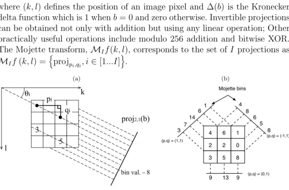
where (k, l) defines the position of an image pixel and ∆(b) is the Kronecker delta function which is 1 when b = 0 and zero otherwise. Invertible projections can be obtained not only with addition but using any linear operation; Other practically useful operations include modulo 256 addition and bitwise XOR.

The Mojette transform, MIf (k, l), corresponds to the set of I projections as

MIf (k, l) = n projpi,qi, i ∈ [1...I] o . (a) k l proj2,1(b) 0i 3 5 bin val. = 8 qi pi (b) 4 6 1 2 2 0 3 5 8 3 7 14 6 1 4 8 6 5 8 9 13 9 Mojette bins (p,q) = (1,1) (p,q) = (0,1) (p,q) = (-1,1)

Fig. 1. (a) A depiction of (pi, qi), the corresponding angle, θi, and the method of

projection, i.e., summing pixel values centered on the line to give a bin value. (b) An invertible Mojette transform of a 3 × 3 example image using direction vectors {(1, 0), (1, 1), (−1, 1)}. Note the spacing between adjacent line sums varies with projection angle

As depicted for the example images in Fig. 1a and 1b, each bin value equals the sum of the pixels crossed by the appropriate line

b = lpi− kqi, (2)

The principle difference from the classical Radon transform is the sampling rate on each projection, which is no longer constant but depends on the

chosen angle as 1/qp2

i + q2i. This can be seen for the different projections

in Fig. 1b which demonstrates the Mojette transform for the directions set

S = {(1, 0) (−1, 1) and (1, 1)}. The number of bins, Bi, for each projection

depends on the chosen direction vector (pi, qi), and for a P × Q image is found

as

Bi = (Q − 1)|pi| + (P − 1)qi+ 1. (3)

The algorithmic complexity of the Mojette transform for a P × Q image with I projections is O(P QI).

2.2 Conditions for reconstructability

Since the set of projection directions is selected arbitrarily, the original data cannot necessarily be recovered from the set of projections chosen. A crite-rion is required to determine if a set of projections is sufficient to uniquely reconstruct the data.

The first result on the conditions for the existence of a unique reconstruction from a given set of I projections came from Katz [13] in a very similar context. He showed that if the following criterion is satisfied, any rectangular P × Q dataset can be uniquely reconstructed:

P ≤ I X i=1 |pi| or Q ≤ I X i=1 qi, (4)

This result has been extended in an independent manner by Normand and Gu´edon [14] to apply to data with compact support of any shape.

2.3 Reconstruction from Mojette projections

The inverse Mojette transform is a fast and simple algorithm [14]. Searching for and updating 1-1 pixel-bin correspondence enables a simple iterative pro-cedure to recover the image. The bin value is back-projected into the pixel and subtracted from the corresponding bins in all other projections. The number of pixels belonging to the corresponding bins is also decremented. The algo-rithmic complexity of the inverse Mojette transform for a P × Q image with I projections is O(P QI) [14]. Figure 2 shows one possibility of the first three steps of the inverse Mojette transform of the example projections given in Fig. 1. 3 37 146 1 4₈ 6-3 =3 5 8 9 -3 =6 13 9 (-1,1) (0,1) (1,1) 1 3 07 146 1 4₈ 3-1 =2 5 8 6 ₁₃ 9 -1 =8 4 1 3 07 1₄ -4 =1 0 6 0 4₈ 2 5 8 6 -4 =2 13 8

...

Fig. 2. Three first possible steps of the inverse Mojette transform of the projections obtained in Fig. 1.

need to search for 1-1 pixel-bin correspondence was removed. It was proven

that when ordered by angle, θi = tan−1(qi/pi), each projection reconstructs

the subsequent qi rows of the image for the case where Pqi = Q (or

subse-quent |pi| columns where P|pi| = P ). This knowledge enables the periodic

sequence of reconstructible pixels to be predetermined, removing the need for the accounting images in the reconstruction.

This result improves reconstruction time by a factor of 5 but is also useful for removing unwanted redundancy. Since the rows (or columns) of the image that are reconstructed by a given projection are known, any projection bins not containing pixels from these rows (or columns) can be removed. Thus for pure compression applications, the Mojette transform can be completely non-redundant mapping P × Q pixels to P Q bins.

3 A review of the preliminary study

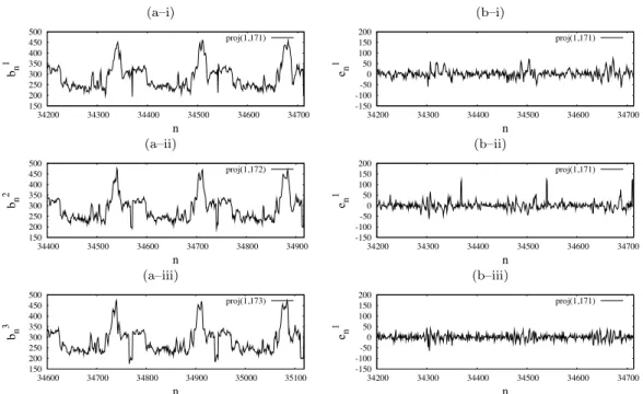
Autrusseau et al [2] noted that the Mojette projection data is highly corre-lated within a projection and also that a strong correlation exists between projections at similar angles. This can be seen in Fig 3a–i to 3a–iii for the projection set {(1, 171), (1, 172), (1, 173)} with respective projection angles of

89.665◦_{, 89.667}◦_{, and 89.669}◦_{. This implies that a form of differential coding}

should be an efficient compression technique.

The technique presented in the paper defines a simple compression technique based on two Differential Pulse Code Modulation (DPCM) schemes of order 1. One scheme is applied within a projection, defined as “intra-projection” cod-ing, and the other is applied between projections, defined as “inter-projection” coding.

Let bi

n denote the value of the nth bin of the ith projection, i.e., projpi,qi(n).

Assume this is the current bin value to be coded and letbbi

n be the prediction

of bi

n with the encoded prediction error defined as ein= bin−bbin.

According to (2), horizontally adjacent pixels in the image are separated by

qi in the projection bins. Therefore the projection data is periodic with qi and

an appropriate prediction for intra-projection coding is:

b

bin= b i

n−qi. (5)

Figure 3b–i depicts the result of this coding applied to the section of proj1,171

given in Fig. 3a–ii. A prediction for inter-projection coding is simply defined as b bi n=eb i+1 n , (6)

(a–i) 150 200 250 300 350 400 450 500 34200 34300 34400 34500 34600 34700 bn 1 n proj(1,171) (a–ii) 150 200 250 300 350 400 450 500 34400 34500 34600 34700 34800 34900 bn 2 n proj(1,172) (a–iii) 150 200 250 300 350 400 450 500 34600 34700 34800 34900 35000 35100 bn 3 n proj(1,173) (b–i) -150 -100 -50 0 50 100 150 200 34200 34300 34400 34500 34600 34700 en 1 n proj(1,171) (b–ii) -150 -100 -50 0 50 100 150 200 34200 34300 34400 34500 34600 34700 en 1 n proj(1,171) (b–iii) -150 -100 -50 0 50 100 150 200 34200 34300 34400 34500 34600 34700 en 1 n proj(1,171)

Fig. 3. (a) A zoom of three projections of ‘Lena’ with projection vectors (1, qi) where

qi is i–171, ii–172, and iii–173 showing the periodicity within a projection and the

correlation between the projections. (b) i–intra-projection coding applied to the section of proj1,171 given in (a–i). ii– inter-projection coding using proj 1,172 (a–ii)

as a reference projection. iii– both intra- and inter-projection coding of proj1,171

where ebi+1

n is the bin in projpi+1,qi+1 that “best” corresponds to b

i

n. This is

more difficult to realise in practice since the projections are of different length and the most appropriate bin to utilise for prediction is not obvious. This is explored more fully in section 4, here linear interpolation is used. Figure 3b–ii

depicts the result of this coding applied to the section of proj1,171given in Fig.

3a–ii using proj1,172 as the reference projection. Both schemes used together

produce a DPCM of order 3 as follows:

b bi n= b i n−qi+eb i+1 n −ebi+1n−qi+1. (7)

Figure 3b–iii shows the result of this coding applied to the section of proj1,171

given in Fig. 3a–ii once again using proj1,172 as the reference projection.

It is important to note that given I projections, the total number of bins

according to (3) is I + (Q − 1)P|pi| + (P − 1)Pqi and Katz criterion, (4),

must be satisfied for inversion. This implies projection sets that minimise

redundancy are those of the form {(1, q1, 1), (1, q2), ..., (1, qI)} such that Pqi

is equal to or only slightly greater than Q (or {(p1, 1), (p2, 1), ..., (pI, 1)} such

that P|pi| ≥ P ). In a compression context, this restriction is more dominant

than selecting projection directions according to texture orientation. A method to take advantage of this is a subject for future research.

im-ages has been presented in Fig. 4. Compression results have been given as the final entropy in bits per pixel (bpp) and have been compared with the original entropy of the image and the compression results from applying JPEG2000. JPEG2000 has been selected for comparison even though it does not generally give optimal compression. It is robust to image type, (i.e., natural, artificial, smooth, textured), and is commonly used due to its multi-resolutional ca-pabilities. Likewise, the Mojette also has other capabilities in data storage and encryption so achieving compression at least comparable to JPEG2000 is desirable.

(a) (b)

Fig. 4. (a) The compression results for Intra- and Inter-projection compression for two projections as outlined in [2] compared with JPEG2000 for the 11 test images depicted in (b) numbered left to right, top to bottom. The first row contains 512×512 natural images: ‘Lena’, ‘Boats’, ‘Peppers’. The second row contains C2RMF images: ‘Hand’ 1200×1854, ‘Drape’ 2376×3542, ‘Flowers’ 1405×1125, ‘Kitchen’ 3822×3333. The last row contains 256 × 256 medical images: ‘Knee’,‘Angio’, ‘MRI’, ‘Chest’

Figure 4 shows that some degree of compression is generally achieved (apart from the high contrast ‘Knee’ image) however the results are not comparable to those from JPEG2000. The next section seeks to identify more powerful prediction schemes which are appropriate for both intra- and inter-projection coding to improve compression results.

4 Projection compression using multi-band image techniques

4.1 Intra-Projection compression of projection images

Phillip´e and Gu´edon [16] showed that the 2D image auto-correlation is retained in the Mojette projections. If the projection data is arranged in columns of

length qi or rows of length pi (whichever is greater is preferable), this

auto-correlation becomes apparent as the projection appears as a “folded” im-age. This has been depicted in Fig. 5 for three projections of ‘Lena’. The

(a–i) 0 100 200 300 400 500 600 700 800 0 10000 20000 30000 40000 50000 60000 70000 80000 bn 1 n proj(1,171) (a–ii) 0 100 200 300 400 500 600 700 800 0 10000 20000 30000 40000 50000 60000 70000 80000 bn 2 n proj(1,172) (a–iii) 0 100 200 300 400 500 600 700 800 0 10000 20000 30000 40000 50000 60000 70000 80000 bn 3 n proj(1,173) (b–i) (b–ii) (b–iii)

Fig. 5. (a) Three 1D projections of ‘Lena’ with projection vectors (1, qi) where qi

is i–171, ii–172, and iii–173 (b) The same projection data displayed as images with columns heights of qi and a width of 514

remapping of projection bins is performed by projecting pixel value, I(k, l), to projpi,qi(nk, nl) according to:

if |pi| ≥ qi      nk = j k |pi| k nl = l − (k−n_pik)qi , otherwise      nl= j l |qi| k nk = k − (l−n_qil)pi , (8)

(where ⌊x⌋ gives the greatest integer less than or equal x), such that the

corresponding bin in the 1D projection, projpi,qi(b), is found as:

b = nlpi− nkqi (9)

This implies that 2D image compression schemes can be applied when per-forming intra-projection coding. The prediction complexity can be increased from a simple DPCM of order 1 to DPCM order to 3 and further to well known ADPCM techniques with context coding such as LOCO (of order 3) [17] and CALIC (of order 7) [18] and Glicbawls [19] which uses the entire set of causal data. As an example, the compression results in bits per pixel (bpp) for each of these respective methods to encode 2 projections of three different images using the direction vectors {(P/2, 1), (P/2+1, 1)} is given in Fig. 6 and compared with the result of applying JPEG2000 to the image. (Similar results are achieved using the direction vectors {(1, Q/2), (1, Q/2 + 1)}). This shows

that compression results better than JPEG2000 can be achieved in some cases with the use of more sophisticated image coding techniques without the need for inter-projection coding. This is an important result for distributed storage. However, the more complex techniques require more memory and computation time. A good trade-off (by design) is CALIC.

0 1 2 3 4 5 6 7 8 1 2 3 4 5 6 7 ent ropy (bpp) Boats Flowers Angio J P E G 2000 CA L IC D P CM -1 D P CM -3 L O CO -I CA L IC G li c ba w ls Applied to 2 proj. 'images' Applied to image

Fig. 6. The entropy results for Intra-projection compression of two projection ‘im-ages’ using prediction schemes: DPCM-1, DPCM-3, LOCO, CALIC, and Glicbawls. This is compared with applying JPEG2000 and CALIC directly to the image

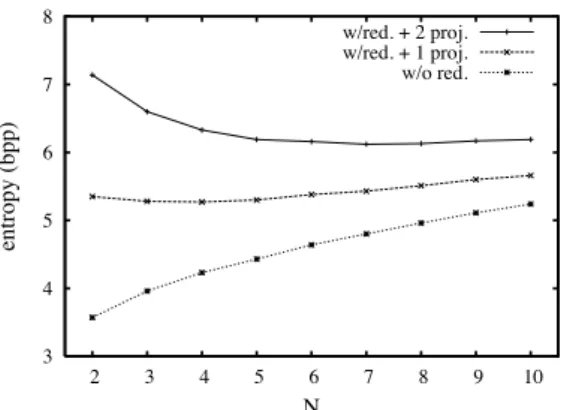
The implications of these results is that redundancy can be inserted for dis-tributed storage or transmission very efficiently. For the example above, an extra projection with a direction vector (−P/2 − 1, 1) can be also included. The resulting compression will still be less than 6.0 bpp (as shown in Fig. 7 for ‘Flowers’) but with the added advantage that any 2 of the 3 projections is sufficient to recover the image according to (4). If each projection is stored on a unique server or transmitted over a unique channel, this is a very se-cure distribution scheme. Of course the number of projections required for reconstruction and the degree of redundancy can be tuned as required. Figure 7 gives the compression achieved with the number of projections re-quired to recover the ‘Flowers’ image, N . At each N there are three values, the first is the compression attained without redundancy in the projections, i.e., N projections. The next two give the compression attained with some redundancy, where 1 (resp. 2) extra projection(s) are included such that any N of the N + 1 (resp. N + 2) projections is sufficient to recover the image, i.e., an additional redundancy of 1/N (resp. 2/N ).

Since the projections can be represented as images, inter-projection coding could be considered to be similar to inter-band image coding, e.g., coding between the RGB components of an image. The next section investigates inter-projection compression issues and techniques associated with this idea.

3 4 5 6 7 8 2 3 4 5 6 7 8 9 10 ent ropy (bpp) N w/red. + 2 proj. w/red. + 1 proj. w/o red.

Fig. 7. A plot of compression against the number of projections, N , required to reconstruct the ‘Flowers’ image: without redundancy, with 1 extra projection (so any N of the N + 1 projections is sufficient for reconstruction), and with 2 extra projections (so any N of the N + 2 projections is sufficient for reconstruction).

4.2 Inter-Projection compression

A simple but effective inter-band prediction method is presented in [20] to extend CALIC to multi-spectral images. The essential idea is to compute the

cross-correlation between the current band, xi_{, and the next band, x}i+1_{, over}

the causal ‘neighbourhood’ data used in CALIC prediction. These regions are

depicted in Fig. 8; Note that xi

n and xi+1n have the same spatial location but

are in different bands. If these two regions are highly correlated then the

intra-band CALIC prediction of the nth _{pixel value of the current band, xb}i

n, can be

improved upon by using information from the next band, xi+1_{. This is true}

since the actual value of the nth _{pixel in the reference band, x}i+1

n , is known. xi n xi+1n xi n-1 ... xi+1 n-1 ...

Current band, i Reference band, i+1

Fig. 8. The causal ‘neighbourhood’ in both the current spectral band and the ref-erence spectral band used in Inter-band CALIC prediction

A similar idea can be applied between Mojette projections of an image. In Inter-band CALIC the different bands contain images that are spatially con-sistent but with different intensities according to the band of the spectrum. With inter-projection compression however, the same pixel intensities, i.e., f (k, l), exist in all projections but with a different phase or period of “mix-ing” with other intensities. Therefore, the best phase to use when predicting

each bin value must be determined. In other words, which projection, projpj,qj,

should be used as the reference projection and which bin in this projection best corresponds to the current bin required to be predicted in the current

projection, proj_pi,qi?

Let us investigate the position of pixels summed in a “raysum” to give a

bin value, proj_pi,qi(b). Adjacent pixels in this set are separated by (pi, qi) as

shown in Fig. 9a. Consider the pixels sampled by two raysums from different projections as depicted in Fig. 9b. This figure shows that the distance between

the previous and subsequent pixels sampled increases by (pi− pj, qi− qj) each

step. Therefore when coding projpi,qi the obvious choice of projection to utilise

as a reference for inter-projection compression is projpj,qj such that the length

of this difference vector is minimised. This is denoted as proj_pi+1,qi+1.

The question of which raysum from this projection should be used for predic-tion of bi

n = projpi,qi(n) is not so obvious since it is more content dependant. A

selection criterion is required to determine the best raysum from projpi+1,qi+1

in the shaded region of Fig. 9c that will give the best prediction for the ray-sum, bi

n, shown. There are two questions: 1. How many candidate raysums are

there in projpi+1,qi+1? and 2. What are their bin indices?

(a) pi qi (b) 3(pi-pj,qi-qj) 2(pi-pj,qi-qj) (pi-pj,qi-qj) (c)

Fig. 9. (a) Relative position of pixel values summed to give a projection bin value. (b) The difference in sampled pixels between two raysums of different projections including a common pixel. (c) The shaded region contains raysums from proj_pj,qj that intersect the given raysum from proj_pi,qi whose contibuting pixels are shown as white squares

To address the first question, assume there are a maximum of ri image pixels

sampled in the raysum to give bi

n. The value of riis found as min(⌈P/pi⌉, ⌈Q/qi⌉)

where ⌈x⌉ gives the smallest integer greater than or equal x. The longest pos-sible vector between corresponding sampled pixels of the two lines is therefore

(ri− 1)(pi− pi+1, qi− qi+1). This also gives the maximum possible vector

be-tween pixels on the two bounding lines in Fig. 9c. Thus, from (2) there are

M = (r − 1) [(qi− qi+1)pi+1− (pi− pi+1)qi+1] + 1 candidate raysums in the

shaded region of Fig. 9c. For this example assume M = 5 as shown in Fig. 10a.

To determine the indices of these candidate bins is straight forward. The raysum that samples pixels closest to the l axis (dark grey pixels in Fig. 10a)

intersects with the the raysum giving bi

n (white pixels in Fig. 10a) in first

region of the image, m = 0, as indicated in Fig. 11a. Therefore, the (nk, nl)

(a) proj(pi,qi) proj(pi+1,qi+1) bi n bi+1 n-m m = 0 m = 1 m = 2 m = 3 m = 4 (b) proj(pi,qi) proj(pi+1,qi+1)

b

b

Fig. 10. (a) Depiction of the 5 candidate raysums from proj_pi+1,qi+1 in the shaded region labelled by phase, m. Any of these could be used when predicting the given bin value in proj_pi,qi. (b) the position of these bins in the respective projection ‘images’

in Fig. 10b), i.e.,

e

bi+1_n = projpi+1,qi+1(nlpi+1− nkqi+1), (10)

This is for a set of (pi, qi) direction vectors where |pi| ≥ qi. The same equation

applies to the case where |pi| < qi, however, here it is the raysum the samples

pixels closest to the k axis, (black pixels in Fig. 10a).

In summary, the bin values from projpi+1,qi+1 that are candidates to be used in

the prediction of bi

n includeebi+1n from (10) and the preceding M − 1 bin values,

i.e., ebi+1

n−m for m ∈ [0, M − 1]. These bins have been depicted in Fig. 10b for

the example. Given the optimal candidate bin ‘phase’, m, the intra-projection prediction can be improved by:

b bi n = pred(b i n) +eb i+1 n−m− pred(ebi+1n−m), (11)

where pred() is any of the prediction models introduced in section 4.1. Selecting phase, m, in the reference projection for the prediction, i.e., using

e_bi+1

n−m, gives the best prediction for the mth section of the image, as labelled

in Fig. 11a for the example given in Fig. 10a and 10b. The prediction is successively worse for the regions m ± 1, m ± 2, and so on. A sensible choice for m is therefore the raysum in the centre of the shaded region, M/2, and this does in general give the best result. However, if the central region of the image is smoother than towards the image boundaries, the correct prediction

of texture edge positions is more critical than an overall minimum distance between corresponding sampled pixels of the two raysums.

This has been demonstrated for several 512 × 512 images using the proj104,1

to predict projection proj_103,1. In this case, (as in the previous diagrams),

there are M = 5 candidate raysums to investigate which correspond to the 5 sections of the image as shown in Fig. 11a. In these regions the sampled

pixels of the raysums from bi

n and ebi+1n−m are identical (and hence the data

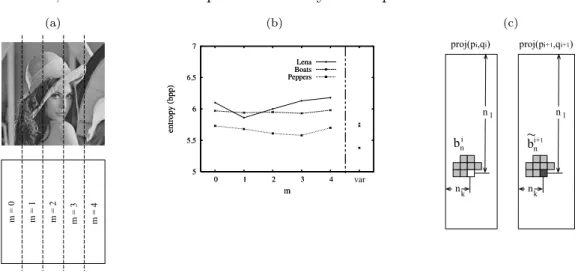
of these sections is removed entirely according to (11)). Figure 11b gives the inter-projection compression rates achieved using (11) with constant phase, m, for all predictions. Here pred() is the Gradient Adjusted Prediction (GAP) introduced in [18]. It is expected that these plots attain a minimum at m = 2, however, this is not true in practise for any of the plots.

(a) m = 0 m = 1 m = 2 m = 3 m = 4 (b) 5 5.5 6 6.5 7 0 1 2 3 4 5 ent ropy (bpp) m Lena Boats Peppers 5 5.5 6 6.5 7 0 1 2 3 4 5 ent ropy (bpp) m Lena Boats Peppers var (c) proj(pi,qi) proj(pi+1,qi+1) bi n b i+1 n n n n n k k l l

Fig. 11. (a) the 5 regions of the image which in selecting phase, m, in prediction will be removed entirely from the current projection after coding. (b) The compression results for inter-projection compression of proj103,1 from proj104,1 using constant m

and variable m, i.e., ‘var’. (c) The causal neighbours from the current projection and the reference projection used firstly to determine cross-correlation and also for prediction

By selecting phase, m, the contribution of the mth _{section of the data is}

removed. Thus, better compression results are achieved when the phase cor-responds to the most textured region of the image. For example, the second region of ‘Lena’, labelled m = 1 in Fig. 11a, contains the highly textured hair. Removing this textured region from the projection by setting m = 1 for inter-projection coding gives the lowest entropy as seen in Fig. 11b. These results demonstrate that the accurate location of texture edges is very important in the predictors performance.

A content dependant method is desired to select the optimum raysum from the

M candidate raysums of projpi+1,qi+1. A fast method that attains near optimal

performance in inter-projection coding is to determine the vertical region of

‘activity’ and select the phase ofebi+1

n−m, accordingly.

A slower but more effective selection criteria can be achieved by investigating

the 2D cross-correlation between the causal neighbourhoods of bi

n and ebi+1n−m

in the two projections for all phases, m ∈ [0, M − 1]. These causal neigh-bourhoods have been depicted in Fig. 11c. The phase, m, of the candidate bin selected, ebi+1

n−m, is that with the greatest cross-correlation with bin. If this

cross-correlation is above some threshold it should be useful to improve the intra-projection prediction, otherwise only intra-projection coding is consid-ered. This gives the best overall compression results as shown for the ‘var’ ,(i.e., variable), column in Fig. 11b with compression consistently lower than any constant phase, m.

(a) (b–i) (b–ii) (b–iii)

Fig. 12. (a) The compression results for Inter-(GAP) and Intra-(CALIC) projec-tion compression of two projecprojec-tions using variable phase, m. Compared with the inter-projection compression results from the previous section using scheme B. (b) A visualisation of the decorrelation achieved using inter-projection coding. Three prediction error projections i–proj170,1, ii–proj171,1, and iii–proj172,1 of ‘lena’.

Pro-jections i and ii have been inter-coded and effectively decorrelated from projection iii. Note that the grey levels are centered about 0 with a window of 64.

Figure 12b shows, for the example projections, that inter-projection coded data (12b–i and 12b–ii) has been effectively decorrelated from the basis pro-jection (12b-iii). Figure 12a shows the compression rates using GAP for inter-projection prediction and CALIC for Intra-inter-projection coding are comparable to JPEG2000.

Figures 13a and 13b summarise the results achieved in this paper for intra-and inter-projection coding respectively. They plot the average compression ratios of each type of image, i.e., natural,art, and medical, using the compres-sion techniques from the premiminary study (Fig. 4a), and the multi-spectral band image coding scheme (Fig. 12a). The average entropy of each scheme is compared with the entropy of the original image and the compression achieved

using JPEG2000. Results show that this scheme is particularly suited to the intended application to the scanned art image database of the C2RMF. For the art images, the compression achieved using solely intra-projection coding is similar to JPEG2000 and including inter-projection coding is more effective than JPEG2000.

(a) Intra-projection coding (b)Inter-projection coding

Fig. 13. A plot of average compression ratio over the 11 test images for both (a) intra-and (b) inter-projection coding using: the DPCM-1 method from the preliminary study, and the CALIC image scheme. Results are compared wih the average entropy of the raw image and the compression achieved by applying JPEG2000 to the image.

5 Conclusions and Future Research

The technique to losslessly compress images via linear prediction of the Mo-jette projection presented in [2] has been improved upon here. Average com-pression achieved using intra-projection coding of 2 projections was improved from 5.38 bpp to 4.48 bpp using a fast lossless image coding technique. Average inter-projection compression entropy was also improved from 4.77 bpp to 4.00 bpp using a lossless inter-spectral band image compression technique. Figure 13 shows that these improved results are comparable to those achieved using JPEG2000 applied directly to the image and that these techniques are par-ticularly suited to the intended purpose of this work on compressing scanned art images for the TSAR project.

The image coding techniques have been adapted to fully exploit the nature of the Mojette projection data. This periodic nature is present since the Mojette projections preserve the 2D auto-correlation of the image and implies that image compression and inter-spectral band image compression can be applied. The prediction method selected for intra-projection coding should be selected depending on the requirements for compression and implementation time. A

method to select the optimal raysum from all candidate raysums of a reference projection to use for inter-projection prediction has also been presented. Compression rates comparable to JPEG2000 are achieved using image coding techniques, however, the image coding techniques take advantage of the 2D correlation and hence, by design, have less complexity, require less memory, and thus have a lower implementation time. Another possible compression scheme that may be applicable is video inter-frame coding with motion esti-mation and is a direction for future research. Another area for future investi-gation is that of coding colour images with predictions using inter-projection and inter-band correlation simultaneously.

These results imply that the Mojette projections which have applications in distributed storage and encryption of images in databases can also be ef-fectively losslessly compressed and many of the requirements of an image database outlined in section 1 can be achieved using solely the Mojette trans-form.

The methods explored here concentrated on predictive coding. Techniques using scalable transforms such as DWT, DCT and FFT may prove useful. If a block based approach could be made feasible, then it may also be beneficial to investigate projections directed along and orthogonal to texture orientation.

Acknowledgements

The majority of this work was conducted while AK held a postdoctoral po-sition at l’Universit´e de Nantes supported by a grant from the R´egion Pays de la Loire, France. This work is funded by Region Pays de la Loire - Miles project.

References

[1] JP. Gu´edon, D. Barba and N. Burger, Psychovisual image coding via an exact discrete Radon transform, Proc. Visual Communications & Image Processing (VCIP), Lance T. Wu editor, May 1995, Taipei, Taiwan, pp. 562-572.

[2] F. Autrusseau, B. Parrein and M. Servi`eres, Lossless Compression Based on a Discrete and Exact Radon Transform: A Preliminary Study, Proc. IEEE Int. Conf. on Accoustics, Speech, and Signal Processing (ICASSP), vol. II, May 2006, Toulouse, France, pp. 425-428.

[3] P. Gu´edon, B. Parrein and N. Normand, Internet distributed image information system, Integrated Computer-Aided Engineering, vol. 8, pp. 205-214, 2001.

[4] A. Kingston, S. Colosimo, P. Campisi and F. Autrusseau, Lossless Image Compression and Selective Encryption Using a Discrete Radon Transform, IEEE International Conference on Image Processing, Sept. 16-19 2007, San Antonio, TX, USA.

[5] F. Zhai, Y. Eisenberg and A. K. Katsaggelos, Joint source-channel coding for video communications, Handbook of Image and Video Processing, Elsevier Academics Press, 2nd Edition, Al. Bovik editor, 2005.

[6] G. Davis and J. Danskin, Joint source and channel coding for image transmission over lossy packet networks, SPIE Conference on Wavelet Applications of Digital Image Processing XIX, pp. 376-387, August 1996.

[7] H. Bin, G.F. Elmasry and C.N. Manikopoulos, Joint lossless-source and channel coding using ARQ/go-back-(N, M) for image transmission, IEEE Transactions on Image Processing, 12(12), pp. 1610-1617, Dec. 2003.

[8] Y. Ming and N. Bourbakis, An overview of lossless digital image compression techniques, 48th Midwest Symposium on Circuits and Systems, 2(7-10), pp. 1099-1102, Aug. 2005.

[9] JP. Gu´edon and N. Normand, The Mojette Transform: the First Ten Years, Proc. 12th International Conference on Discrete Geometry for Computer Imagery,

´

E. Andres and G. Damiand and P. Lienhardt editors, Springer-Verlag, vol. LNCS3429, pp. 79-91, Poitiers, France, Apr. 2005.

[10] SR. Deans, The Radon Transform and Some of Its Applications, revised edition, Krieger, Malabar, FL, 1993.

[11] F. Mat´uˇs and J. Flusser, Image representation via a finite Radon transform, IEEE Transactions on Pattern Analysis & Machine Intelligence, 15(10), pp. 996-1006, Oct. 1993.

[12] BT. Kelley and VK. Madisetti, The fast discrete Radon transform. I: Theory, IEEE Transactions on Image Processing, 2(3), pp. 382400, 1993.

[13] M. Katz, Questions of uniqueness and resolution in reconstruction from projections, Lect. Notes in Biomath., Springer Verlag, 1977.

[14] N. Normand, JP. Gu´edon, O. Philipp´e and D. Barba, Controlled redundancy for image coding and high-speed transmission, Proc. SPIE Visual Communications and Image Processing, R. Ansari and MJ. Smith editors, vol. 2727, pp. 1070-81, Feb. 1996.

[15] N. Normand, A. Kingston and P. ´Evenou, A Geometry Driven Reconstruction Algorithm for the Mojette transform, Proc. 13th International Conference on Discrete Geometry for Computer Imagery, A. Kuba and LG. Ny´ul and K. Pal´agyi editors, Springer-Verlag LNCS4245, pp. 122-33, Szeged, Hungary, Oct. 2006. [16] O. Philipp´e and JP. Gu´edon, Correlation of the Mojette representation for

non-exact image reconstruction, roceedings of Picture Coding Symposium, vol. 1, pp. 237-41, Berlin, Germany, Sep. 1997.

[17] M.J. Weinberger and G. Seroussi and G. Sapiro, LOCO-I: a low complexity, context-based, lossless image compression algorithm, Proc. Data Compression Conference, IEEE Computer Society, Mar - Apr 1996, pp 140-149, Los Alamitos, CA, USA.

[18] X. Wu and N. Memon, Context-based, adaptive, lossless image coding, IEEE Transactions on Communications, 45(4), pp. 437-444, Apr 1997.

[19] B. Meyer and P. Tischer, Glicbawls - Grey Level Image Compression by Adaptive Weighted Least Squares, IEEE Computer Society, Proc. Data Compression Conference, pp. 503, Snowbird, Utah, USA, Mar. 2001.

[20] X. Wu and N. Memon, Context-based lossless interband compression-extending CALIC, IEEE Transactions on Image Processing, 9(6), pp. 994-1001, Jun. 2000.