HAL Id: hal-01699865
https://hal.archives-ouvertes.fr/hal-01699865
Submitted on 2 Feb 2018
HAL is a multi-disciplinary open access
archive for the deposit and dissemination of
sci-entific research documents, whether they are
pub-lished or not. The documents may come from
teaching and research institutions in France or
abroad, or from public or private research centers.
L’archive ouverte pluridisciplinaire HAL, est
destinée au dépôt et à la diffusion de documents
scientifiques de niveau recherche, publiés ou non,
émanant des établissements d’enseignement et de
recherche français ou étrangers, des laboratoires
publics ou privés.
Controller design for a class of delayed and constrained
systems. Application to supply chains
Charifa Moussaoui, Rosa Abbou, Jean-Jacques Loiseau
To cite this version:
Charifa Moussaoui, Rosa Abbou, Jean-Jacques Loiseau. Controller design for a class of delayed and
constrained systems. Application to supply chains. A. Seuret; H. Özbay; C. Bonnet; H. Mounier.
Low-Complexity Controllers for Time-Delay Systems, 2, Springer, 2014, Advances in Delays and Dynamics.
�hal-01699865�
constrained systems. Application to supply
chains.
Charifa Moussaoui, Rosa Abbou and Jean Jacques Loiseau
AbstractThis chapter aims to investigate the construction of efficient controllers for some input time delay systems, subjected to strict constraints of positivity and saturating limitations, in presence of some exogenous bounded disturbances. The results are presented through the application of supply chains, for which controller design is a challenging issue trading-off between stabilising properties in presence of time lags, and constraints due to the physical limitations and specificities of the plants of the supply chain. We show that the stabilization of such flow systems can be tackled by the stabilization of input time delay systems, using a predictor based feedback approach. This classical control method, which permits to overcome the delays, is enriched by using saturation terms that allow the consideration of the physical constraints of the system resources composing the serial supply chains.
1 Introduction
Input time delay systems are common models widely used for dead-time systems representation. Such systems are characterized by the presence of some irreducible time lags, due to, for example, process durations, mass or information transport phenomena and sensor responses. These systems attracted a great deal of attention from both practitioners and researchers, since they are involved in many industrial processes and applications. The control problems related to are challenging issues which fuel constantly the researchers community. Indeed, in addition to the pres-ence of time-lags, these systems are frequently subject to some physical constraints and additional specificities. Furthermore, they are often subject to some exogenous perturbations effects, that makes the controller design task quite more difficult.
Charifa Moussaoui, Rosa Abbou and Jean Jacques Loiseau
LUNAM Universit´e, Institut de Recherche en Communications et Cybern´etique de Nantes, UMR 6397. ´Ecole Centrale de Nantes, 1 rue de la No¨e, BP 92101, 44321 Nantes Cedex 3, FRANCE. e-mail:{Charifa.Moussaoui, Rosa.Abbou, Jean-Jacques.Loiseau}@irccyn.ec-nantes.fr
Our concerns focus on the supply lines supply lines which are quite representa-tive of such dead-time systems. They consist of a network of interconnected stages, composed of manufacturers, suppliers parts, exchanging goods, financial and infor-mation flows, through transportation, warehousing and retailing operations, all in the sake of fulfilling end-customer requests. These operations are time consuming and request important time-lags that can not be neglected or simply approximated. A central issue is to coordinate them over different stages and locations, while provid-ing a convenient service level to end-customers. This task is quietly enhanced when the market demands are unstable or unknown in advance. In addition, the supply line resources are limited by the storage and the production or supplying capacities, which are current bottlenecks for the system. Indeed, the storage devices, say the inventories, are finite resources that can be subject to congestion problems which lead to important goods losses, while the production units are subject to saturation phenomena due to actuator limitations. These practical problems are commonly performed in other systems, where the dynamics is governed by constrained flow exchanges, such as the communication networks and some others load-balancing systems, where the information flows and the buffers in the network nodes, can be perceived, respectively, as the good flows and the inventories of a supply line.
In this chapter, supply line control issue is formulated as a general constrained control problem, for input time delay systems with positivity constraints and satu-rated resources, subject to unknown but bounded disturbances. To handle this prob-lem, we make use of predictive-based control techniques, which efficiency in com-pensating the input time delay is well-established and widely described in the liter-ature. Using pole assignment principle and model reduction [1, 12, 13], we propose a saturated and constrained control law, which allows the controller to handle the system constraints and to meet its specifications. The proposed methodology for designing such controller consists in defining an invariant set for the system tra-jectories, such that the bounded input bounded output (BIBO) stability property is ensured, and for which the system constraints are meet.
After introducing the problematic, the chapter is organized as follows. In Section 2, the dynamical model of each stage of the considered supply line is proposed, and a quick review of the literature concerning this topic is presented. Section 3 is devoted to the controller structure, where some backgrounds about saturated commands and the predictive control methods for input time delay systems are presented. In Sec-tion 4, the controller design issues are addressed and these results are extended to the case of a multi-level supply line in the Section 5, and illustrated through an nu-merical example in Section 6. Finally, a discussion about the obtained results and further investigations conclude this chapter.
2 Problem statement: Inventory and production control
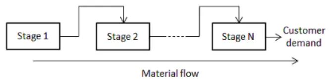
A supply line is a series of stages or levels, that represents manufacturers, suppli-ers, transporters and other parts that are involved in supplying process, in which the
goods flow linearly to reach end-customers, as depicted in Figure 1.
Fig. 1 Multi stages supply chain scheme.
Supply chain control consists of defining appropriate ordering policies that regu-late the production and the supply rates in the different stages of the supply line, so that each stage is able to meet the inventories requirements, and to provide a good service level for the incoming demands. In this field, different frameworks where proposed during the past decades, based on optimization procedures using programming techniques, empirical experiences and control theory methods. Our concern focused on the use of the control theory methods, which provide an ana-lytical and formal framework and allow a structural approach to handle the supply chain issues. Indeed, since the pioneering works of Simon [18], who was the first to use Laplace transform to analyze a supply line dynamics, numerous investigations followed, such that [6, 24, 5, 22, 15, 26], in which the supply chain was modelled us-ing block diagrams and controlled through feedback structures. These investigations lead to the well-known Automatic Pipeline Inventory and Order Based Production Control System (APIOBPCS) models and their variations [10]. They permit to un-derstand the complex interactions that govern supply chains dynamics, identifying the critical agents that impact the inventories stability, such that the delays. The au-thors highlighted the importance of the Work In Process (WIP), which is the amount of goods ordered in the pipeline but not yet received due to the delay. They also re-veal its central role in damping the variance of the demand amplification among the supply chain stages, which is known as the bullwhip or Forrester effect [6].
The advances in the time delay systems control [14, 21], allow further insights into the delayed differential equations describing , in particular, the inventory dy-namics [25, 19, 4], and notable works like [20] permit great extensions considering multiple delays. Nevertheless, the aforementioned works did not take into account the positivity and the capacity constraints of the supply chain resources. Actually, both inventory levels and replenishment orders are constraint free, and are allowed to get some negative values or excessive huge ones, which does not correspond to real plant capacities and thus creates a major gap between theoretical attempts and practical results. For such issues, simulation based analyses are the mostly used, such as in [3, 7, 8, 29, 2, 17], where the impact of constrained production capacity is studied. In [27, 28] an analytical investigation is presented for the forbidden-return case, which corresponds to the constraint of non-negativity on the replenishment orders only. These studies pointed out that considering capacity constrained on the supplying devices, removes the linearity assumption of the model and hence
com-plex dynamics behaviours are revealed. To the best of our knowledge, no work in this field considers capacity and positivity constraints, on both the supplying devices and the inventories, taking into account the pure delays present in these systems dy-namics. This is what this work contributes to. We consider a multi-stage supply line. In a first attempt, our analysis will be held for a single stage, the general case will be presented in Section 5.
Each stage of the supply line represents an elementary system composed of a supplying unit and a storage one. The term ”supplying” is used for the operations of material acquisition, which can be production, transport or retailing process. The supplying units are characterized by a delayθwhich corresponds to the time needed to complete the supplying task, and to a supplying order rate denoted u(t), which is limited by a maximum supplying capacity denoted Umax. The storage units are
namely the inventories. Each elementary stage of the supply chain has an inventory with a maximum storage capacity denoted Ymax. In this work, the customer demands
are unknown in advance but assumed to be upper bounded by an amount denoted dmax. The generic model for the inventory level dynamics is then described by the
following first order delayed equation.
˙ y(t) =
{
u(t−θ)− d(t) for t ≥θ
ϕ(t)− d(t) for 0≤ t <θ, (1) where, y(t) is the inventory level and d(t) the incoming demand rate of each level. The functionϕ(t) describes the initial state of the system such that equation (1) de-scribes the initial dynamics of the inventory for 0≤ t <θ.
As already mentioned, supplying units and inventories as well, are limited resources, which can take non-negative values only. These constraints are formulated as fol-lows. For inventory level
y(t)∈ [0,Ymax] , for t≥ 0, (2)
and for the supplying rate
u(t)∈ [0,Umax] , for t≥ 0. (3)
Then, the working assumption on the consumer demand is formulated such as d(t)∈ [0,dmax] , for t≥ 0. (4)
The controller design task consists of defining a controller which will stabilize the delayed system (1) while ensuring the fulfilment of the constraints (2) and (3), for every bounded disturbance verifying the assumption (4).
3 System control structure
A local management strategy is used for the elementary level, which aims at meeting its local specifications. In this work, we consider that all stages of the considered supply line are applying the same ordering rules, which consists of fulfilling on line the consumer demands, and replenishing the inventory to a referential level denoted yc. The strategy to define on line the control law, that is the supplying rate at each
level of the supply chain, is presented in the following section.
3.1 Order rates and control structure
The order rate u(t) at a given level represents the command of the delayed system given by equations (1). Regarding to the system constraints, and the nature of the system, the control law we propose to apply is a saturated command based on a feedback predictor structure such that
u(t) = sat [0,Umax]
[K(yc− z(t))] ,for t ≥ 0. (5)
where ycis the reference signal of the system, which corresponds to the reference
level for the inventory. K is the controller gain which is used to adjust the order rates placed in each level, and z(t) is the prediction of the future state of the system, that corresponds to the inventory level at t +θ, as it is shown in the sequel.
Saturated commands are commonly used for systems with saturating actuators, and permit to take into account theirs specific limitations. It was shown to be more effi-cient and realistic than a linear constraint control [23, 9]. On the other hand, the use of a saturated controller introduces non-linearities in the closed-loop scheme of the system, due to the sat function defined as
sat [a,b] [ f (t)] = b if f (t) > b , f (t) if a≤ f (t) ≤ b, a if f (t) < a .
For such non-linear systems, stability conditions can be obtained by computing in-variant sets in which the system trajectory remains, and in which the saturation constraints are met, as it is shown in the sequel. The feedback predictor part of the command, is used to handle the delays and the stability properties of the infinite-dimensional system, by allowing the assignment of the closed-loop system poles, in a finite number of locations in the complex plan [12, 11]. Also known as model reduction or Artstein reduction [1], the basic idea of state prediction is to compen-sate the time delayθby generating a control law that enables one to directly use the corresponding delay-free system, thanks to the prediction defined by
z(t) = {
y(t) +∫t−t θu(τ)dτ for t≥θ,
y(t) +∫tθϕ(τ)dτ+∫0tu(τ)dτ for t <θ, (6) which can be rewritten, using expression (1) as
z(t) = y(t +θ) +
∫ t+θ t
d(τ)dτ, for t≥ 0. (7) Indeed, by time derivation of this equation (7), one can see that the resulting system ˙z(t) = u(t)− d(t) ,for t ≥ 0, (8) is delay-free. The system (8) is the reduced model of the system (1)-(5). Artstein [1] demonstrated that the control low u(t) is admissible for the closed loop system (1)-(5) if and only if it is admissible for the system (8)-(5), and that the two systems have the same dynamics properties. Our approach is then based on the use of the reduced system (8) to design the controller such that the system constraints and requirements (2) and (3) will be fully met, as shown in Section 3.2.
3.2 The closed-loop system dynamics
The dynamics of the closed-loop system (8)-(5) is given by the following expression. ˙z(t) = sat
[0,Umax]
[K(yc− z(t)] − d(t) , for t ≥ 0. (9)
The stability analysis of this system is performed by computing an invariant inter-val for the trajectories of system (9), in which the system constraints are met, and the BIBO stability property of the system is warranted. In this sake, the system con-straints (2) and (3) are reformulated in terms of the new state variable z(t) as follows. Using the expression (7), one can see that
y(t +θ) = z(t)−
∫ t+θ
t
d(τ)dτ, t≥ 0. (10) The constraint (2) is verified if both z(t) and the term∫tt+θd(τ)dτ are bounded, so that y(t +θ) ∈ [0, Ymax]. Provided condition (4) is satisfied, it is seen that
∫t+θ
t d(τ)dτ∈ [0,θdmax] ,∀t ≥ 0. Thus, z(t) should be limited by a lower and an
upper bound, zminand zmaxrespectively, which verifies the relation (10), such that
0≤ zmin−θdmaxfor y(t +θ) = 0 , and zmax≤ Ymaxfor y(t +θ) = Ymax.
Then, the original delayed system verifies y(t)∈ [0,Ymax] for all t≥ 0, if and only if
the condition
withθdmax< Ymax, is verified for the reduced system. The control problem
estab-lished in Section 2, is reformulated in terms of founding the controller parameters, which permits to the closed loop system (8)-(7), to verify the constraints (11) under disturbance effects of d(t). The results are given in Section 4.
3.3 Admissible initial conditions
Non-zero initial conditions does not affect the control structure and the system con-straints. Indeed, as shown by equation (1) for t∈ [0,θ], the inventory level evolution depends on the functionϕ(t) and the demand only. Because of the delay, the effects of the command u(t) on the system dynamics are not visible before t =θ. Then, checking whether the system constraints are met or not on the time interval [0,θ[ yields a set of admissible initial conditions, for which the constraint conditions are verified. This set is characterized as follows. Using equation (1), for 0≤ t <θ, the inventory level is given by
y(t) = y0+ ∫ t 0 ϕ (τ) dτ− ∫ t 0 d(τ) dτ,
where y0 is the initial inventory level at time t = 0, and the amount
∫θ
0 ϕ(τ)dτ represents the initial WIP in the pipeline that is denoted wip0. It is seen that the term∫0td(τ)dτbelonging to the interval [0,θdmax], y(t) verifies y(t)∈ [0,Ymax] for
t∈ [0,θ[ if and only if the initial conditions are such that
θdmax≤ y0+ wip0≤ Ymax.
4 Controller designing issues
The controller design consists in determining suitable gain K and inventory refer-ence level yc for each elementary stage of the supply chain, such that the system
constraints and specifications are fully met.Two main issues are to be considered. First, for given systems parameters, namely the maximum capacities Umaxand Ymax,
is it possible to find a controller which will fully meet the constraints and the sys-tem requirements. Then, if such a controller is indeed feasible, the second issue is about the choice of the command parameters K and ycunder the system constraints
and specifications. This is the parameterization phase. In this section, both issues are treated through the dynamics properties analysis of the system, such that the exact solution of the equation (9) is not required. Our proposal is to determine some necessary and sufficient conditions on the controller parameters, to impose the in-variance property of the interval (11), so that the BIBO stability of the system and the constraints are all satisfied. These conditions are given through the following
Theorem 1. A corollary is then formulated, which gives further results concerning the closed-loop system dynamics under Theorem 1 assumptions.
Theorem 1. Being given a system of the form (1), there exists a command of the form (5), for which the system is stable and the constraints (2) and (3) are fulfilled, for any d(t)∈ [0,dmax] if and only if the following conditions hold true
θdmax< Ymax, (12)
and
dmax≤ Umax. (13)
In addition, if the conditions (12) et (13) are met, the constraints (2) and (3) are satisfied under the control law (5) if an only if the controller parameters are such that:
θdmax+
dmax
K ≤ yc≤ Ymax. (14)
Proof. As shown in Section 3.2, the controller of the reduced system (9) should be designed such that constraint (11) is fulfilled. The existence of the controller is then linked with the non-empty property of interval [θdmax,Ymax], which is true only
whenθdmax< Ymax. This later shows the necessity of condition (12), its sufficiency
being obvious.
Conditions (13) and (14) come from the fact that, verifying constraint (11) at any time t≥ 0 implies that, the closed interval [zmin, zmax] is invariant for the system
trajectories. Formally, this property is warranted if and only if the following impli-cations are true, for all t≥ 0
z(t) = zmin⇒ ˙z(t) ≥ 0, and z(t) = zmax ⇒ ˙z(t) ≤ 0.
Using expression of ˙z(t) given by (9), and provided that (4) is true, these inequalities are rewritten respectively
sat [0,Umax]
[K(yc− zmin)]≥ dmax, (15)
and
sat [0,Umax]
[K(yc− zmax)]≤ 0. (16)
Using the sat function definition given in Section 3.1, one can see that the inequality (15) is solvable if and only if Umax≥ dmax, that shows the sufficiency and necessity
of condition (13), and thus ycis such as zmin+ dmax/K≤ yc, which, together with
condition (12) and the equality zmin=θdmax, establishes the sufficiency of the left
part of the condition (14) of Theorem 1. Its necessity comes form the fact that for yc< zmin+ dmax/K, inequality (15) has no solution.
The same analysis is applied for inequality (16). This latter is solvable if and only if
which, together with equality zmax= Ymaxshows that yc≤ Ymax. This establishes the
sufficiency and the necessity of the right member of condition (14) of Theorem 1,
and completes the proof. ⊓⊔
Under the conditions of Theorem 1, the analysis of the closed-loop system dy-namics shows that the system constraints and specifications are truly met. Any sat-isfactory controller actually permits to fill more restrictive constraints on the system variables. We describe these restrictions in the following corollary.
Corollary 1. Being given a system of the form (1), with a control law of the form (5) and suitable initial conditions, such that the conditions (12), (13) and (14) are verified, then the following holds true
y(t)∈ [ yc− dmax K −θdmax, yc ] , (18) and u(t)∈ [0,dmax] , (19)
for all t≥ 0 and d(t) ∈ [0,dmax].
Proof. From expression (9), one can observes that, under Theorem 1 assumptions, the following implications are true for all t≥ 0,
z(t)≥ yc⇒ ˙z(t) ≤ 0 and z(t) ≤ yc−
dmax
K ⇒ ˙z(t) ≥ 0.
These implications show that the effective interval of variation of z(t) is such that z(t)∈ [ yc− dmax K , yc ] , (20)
which represents the smallest invariant interval for the system (9). Indeed, under Theorem 1 assumptions, it is seen that the interval given in (20) is included in the interval given by (11). Thus, using expressions (10) and (5), one can compute the effective interval of y(t) and u(t) variations which are given by expressions (18) and
(19) respectively. ⊓⊔
5 Generalization for N-stages supply chain
In this section, we propose a generalization of the results presented above for the multi-stages supply line, composed of N elementary stages, as presented in Section 2. Each level is now labelled with a subscript i, with i = 1, .., N. In such serially linked structure, each stage i has one supplier i− 1, and is supposed to support the incoming demand di(t) of the following stage i + 1 such that di(t) = ui+1(t)
which faces the end consumer demand denoted dc(t). The inventory dynamics of
each stage is given by the following equation.
˙ yi(t) =
{
ui(t−θi)− di(t) for t≥θi, ϕi(t)− di(t) for 0≤ t <θi,
(21)
where, yi(t) is the inventory, ui(t) is the acquisition rate with delayθi, and di(t) the
incoming demand, with i = c for the customer demand rates.
The present part aims to define the controller parameters of each stage, such as the end consumer demand dc(t) will be satisfied, and taking into account the local
constraints of each single level, as seen in Section 4, and the additional constraints due to the serial structure as well. The constraints (2) and (3) are generalized as follows. For i = 1 , .. , N, the inventory levels are such that
yi(t)∈ [0,Ymaxi] , for t≥ 0, (22)
and the acquisition rates verify
ui(t)∈ [0,Umaxi] , for t≥ 0. (23)
The additional constraints arising from the network structure are about the incoming demand of each level, where di(t) = ui+1(t) for i = 1 , .. , N− 1, such that
di(t)∈
[
0,Umaxi+1
]
. (24)
For the retailer stage i = N, the incoming demand is the end customer demand dc(t).
It verifies the same assumption (4) namely
dc(t)∈ [0,dmax] . (25)
The same control law as the one presented in Section 3.2 , is used in each stage. It is of the form
ui(t) = sat
[0,Umaxi]
[Ki(yci− zi(t))] for t≥θi, (26)
with yci is the reference level for the inventory yi, Kiis the controller gain which is
used to adjust the order rates placed in level i, and zi(t) is the prediction of the future
state of the system, defined as follows
zi(t) = { yi(t) + ∫t t−θiui(τ) dτ for t≥θi, yi(t) + ∫θi t ϕi(τ) dτ+ ∫t 0ui(τ) dτ for t <θi, (27)
The controller design issue in each stage is addressed as shown in Sections 3 and 4. Using the same arguments basing on the analysis of the reduced model obtained for each stage, Theorems 1 is now extended to the N-stages supply line.
Theorem 2. Being given a supply chain of the form (21), there exists a command of the form (26), for which the system is stable, and fulfilled the constraints (22), (23)
and (24), for any dc(t)∈ [0,dmax] if and only if the following conditions hold true. θidmax < Ymaxi, (28)
and
dmax≤ Umaxi, (29)
for all t≥ 0 and i = 1,..,N. In addition, if conditions (28) and (29) are verified, the constraints (23), (24) and (25) are met for any dc(t)∈ [0,dmax], if and only if the
controller parameters are such that:
θidmax+
dmax
Ki ≤ yci≤ Ymaxi
(30) For all t≥ 0 and i = 1,..,N.
Proof. For the N-stages supply line serially linked, the whole supply line dynamics is driven by the end-costumer demand dc(t). Applying Theorem 1 for the last stage
N of the line, Theorem 2 shows that the orders uN(t) vary in the interval [0, dmax].
Then the linking relation between the supply line stages, where dN−1(t) = uN(t)
shows that actually dN−1(t)∈ [0,dmax]. Thus, by recursion, it is seen that di(t)∈
[0, dmax] for all i = 1, .., N. Using this result, the demonstration of Theorem 2 is
directly derived from the proof of Theorem 1. ⊓⊔
6 Simulation example and discussions
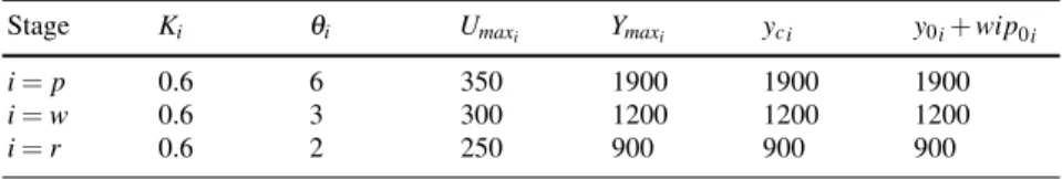
The application example presented in this section, aims at highlighting the efficiency of the distributed control scheme proposed to eliminate the bullwhip effect in a sup-ply chain, and to illustrate the importance of taking into account the positivity and capacity constraints. For this sake, we consider a three-stages supply chain, com-monly used in the literature [3, 8], consisting of a production plant, a wholesale stage, and a distribution centre. Unlike the aforementioned works, where capacity constraints are assumed for the order rates only, we consider both inventories lim-itations, and positivity constraints. The subscripts p , w, and r are used to label the production, the warehouse and the retailer stages respectively. The maximum ca-pacities Umaxi and Ymaxi and some admissible initial conditions are given in Table 1.
Table 1 Simulation parameters for the constrained three-stages supply chain.
Stage Ki θi Umaxi Ymaxi yci y0i+ wip0i
i = p 0.6 6 350 1900 1900 1900
i = w 0.6 3 300 1200 1200 1200
The initial conditions are chosen such that all transitory dynamics are avoided, ac-cording to the rule defined in Section 3.3. Controller parameters Kiand yciare
cal-culated according to Theorem 2, and are also sorted in Table 1. In order to illustrate the inventory dynamics, the customer demand used for this simulation is a square function starting at t = 15 weeks and ending at t = 45 weeks, with an amplitude dmax= 240, unlike the aforementioned works where only step function demands
where considered. The results of the simulation are depicted on Figure 2, where the order rates of each stage and the inventory levels are represented.
Figure 2(a) shows that the order rates placed in each of the three stages, follows closely the demand, causing no amplification through the upstream levels as it is expected by the relation (24). Then, Figure 2(b) shows that the inventory levels re-main non-negative, and are re-completed to their reference levels when the demand is null, as it was specified by the ordering policy presented in Section 1. The out-comes of this simulation study, join the former authors conclusions [8, 29, 2, 3] which stand that capacity constraint of the ordering rates, does not necessarily im-pact the customer service level, which corresponds to the demand satisfaction. The saturating constraint impacts the dynamics too, such that the order rates being lim-ited, the supplying process completion takes more time, but since the condition (29) is verified, the demand is always fulfilled. It is also recognized that such constraints provide an effective improvement in reducing the demand amplification, within the multi-echelon system. Indeed, we showed that a good handling of the delays, via
(a) Dynamics of the order rates
(b) Dynamics of the inventory levels
an appropriate control law, permits to definitely overcome the Forrester effect. This result is also pointed out by the former work of [18] and [16], where it is established that the smoothest system responses are obtained when the same care is given to the inventory discrepancy and the WIP. The formal explanation of this empiric result comes from the input time delay system control, as seen in Section 3, where the ef-ficient delay compensation via the predictor feedback imposes the same coefef-ficient K for both the inventory discrepancy and the distributed delay of the predictor which is the WIP term. Assuming an unknown bounded demand as a working assumption, allows us to maintain this results for every bounded demand signal, no mater if it is a step function shaped or not.
7 Conclusion and perspectives
In this chapter, the controller design problem for serially-linked supply chains, with constrained orders and inventories, and unknown customer demands variations, has been investigated. The problem is stated in terms of controlled input time delay system, with positivity and saturations constraints, subject to bounded disturbances. A saturated feedback predictor controller was introduced to handle both the delayed dynamics and the constraints, where the controller encompasses a distributed delay expressed by the integral term in the prediction. This distributed term corresponds to the WIP amount which the use in inventory regulation is quite classical for damping the bullwhip effect [10, 16, 18]. It is important to notice that the WIP is actually measurable. Thus, the controller proposed in this work is of low complexity, since it corresponds to a static feedback on measurable variables. The main advantage of this work is that practical constraints of positivity and capacity of both orders and inventories are taken into account, that enhanced the accuracy of the results. In addition, the controller proposed eliminates totally the Forrester effect, in case where the delays are properly known. Robustness analysis of the results in case of delay misestimations, and the consideration of variable delays are advised of forthcoming works.
References
1. Artstein, Z.: Linear systems with delayed controls: A reduction. IEEE Transactions on Auto-matic Control. 27 (4): 869–879 (1982)
2. Cannella, S., Ciancimino, E. and Mrquez, A. C.: Capacity constrained supply chains: a sim-ulation study. International Journal of Simsim-ulation and Process Modelling. 4 (2): 139–147 (2008)
3. Evans, G.N. and Naim, M.M.: The dynamics of capacity constrained supply chains. Proceed-ings of International System Dynamics Conference, Stirling, Scotland, 28–35 (1994) 4. Delice, I. I. and Sipahi, R.: Inventory dynamics models of supply chains with delays ;
(eds.) Topics in Time Delay Systems, of Lecture Notes in Control and Information Sciences. Springer, Berlin Heidelberg, 38: 8349–358 (2009)
5. Edghill, J.S., Towill, D.R.: The use of systems dynamics in manufacturing systems. Transac-tion of the Institute of Measurement and Control. (1989) doi: 10.1177/014233128901100406 6. Forrester, J. W.: Industrial Dynamics. Cambridge MA: MIT press, (1961)
7. Gavirneni, S., Kapucinski, R. and Tayur, S.: Value of information in capacitated supply chains, Management Science. 45 (1): 16–24 (1999)
8. Helo, P.T.: Dynamic modelling of surge effect and capacity limitation in supply chains. Inter-national Journal of Production Research. 38 (17): 4521–4533 (2000)
9. Hu,T. L. Z.: Control Systems with Actuator Saturation : Analysis and Design. Birkh¨auser, Boston (2001)
10. John, S., Naim, M.M., Towill, D.R.: Dynamic analysis of a WIP compensated decision sup-port system. International Journal of Management Systems and Design. 1 (4): 283–297 (1994) 11. Kwon, W. and Pearson, A.: Feedback stabilization of linear systems with delayed control.
IEEE Transactions on Automatic Control, 25 (2): 266–269 (1980)
12. Manitius, A. and Olbrot, A.: Finite spectrum assignment problems for systems with delays. IEEE Trans. Automatic Control. 24: 541–553 (1979)
13. Mirkin, L. and Raskin, N.: Every stabilizing dead-time controller has an observer-predictor-based structure. Automatica. 39 (10): 1747–1754 (2003)
14. J. P. Richard, Time-delay systems : an overview of some recent advances and open problems. Automatica. 39 (10):1667–1694 (2003).
15. Riddalls, C.E., Bennett, S. and Tipi, N.S.: Modeling the dynamics of supply chains, Interna-tional Journal of System Science. 31: 969–976 (2000)
16. Riddalls, C. E., et Bennett, S.: The stability of supply chains. International Journal of Produc-tion Research. 40 (2): 459–475 (2002)
17. Shukla, V., Naim, M.M.: The impact of capacity constraints on supply chain dynamics. Inter-national Conference on Computers & Industrial Engineering. CIE 2009, 925–930 (2009) 18. Simon, H. A.: On the application of servomechanism theory in the study of production
con-trol. Econometrica. 20: 247–268 (1952)
19. Sipahi, R., Delice, I.I.: Supply network dynamics and delays; performance, synchronization, stability. Mechanical and Industrial Engineering Faculty Publications (2008) Available at http://works.bepress.com/rsipahi/13
20. Sipahi, R., Delice, I.I.: Stability of Inventory Dynamics in Supply Chains with Three Delays. International Journal of Production Economics. 123: 107–117 (2010)
21. Sipahi, R., Niculescu, S.-I., Abdallah, C. T., Michiels, W. and Gu, K.: Stability and Stabi-lization of Systems with Time Delay, Limitations and opportunities. IEEE Control Systems Magazine. 31 (1): 38–65 (2011)
22. Sterman, J. D.: Modelling managerial behaviour misinterpretations of feedback in a dynamic decision-making experiment. Management Science. 35 (3): 321–339 (1989)
23. Tarbouriech, S., Garcia, G., Da Silva, J., and Queinnec, I.: Stability and Stabilization of Linear Systems with Saturating Actuators. Springer (2011)
24. Towill, D.R.: Dynamic analysis of an inventory and order based production control system. International Journal of Production Research. 20 (6): 671–687 (1982)
25. Warburton, R. D. H.: An exact analytical solution to the production inventory control problem. International Journal of Production Economics. 92: 81–96 (2004)
26. Warburton, R. D. H. , Disney, S. M. , Towill, D. R. and Hodgson, J. P. E.: Further insights into ’the stability of supply chains’. International Journal of Production Research. 42 (3): 639–648 (2004)
27. Wang, X., Disney, S.M. and Wang, J.: Exploring the oscillatory dynamics of a forbidden returns inventory system. International Journal of Production Economics (2012). ISSN 0925– 5273, http://dx.doi.org/10.1016/j.ijpe.2012.08.013.
28. Wang, X., Disney, S.M. and Wang, J.: Stability analysis of constrained inventory systems with transportation delay. European Journal of Operational Research. 223 (1): 86–95 (2012) 29. Wikner, J., Naim, M.M. and Rudberg, M.: Exploiting the order book for mass customized
manufacturing control systems with capacity limitation. IEEE Transactions on Engineering Management. 54 (1): 145–155 (2007)