HAL Id: hal-01044934
https://hal.archives-ouvertes.fr/hal-01044934
Submitted on 24 Jul 2014
HAL is a multi-disciplinary open access
archive for the deposit and dissemination of
sci-entific research documents, whether they are
pub-lished or not. The documents may come from
teaching and research institutions in France or
L’archive ouverte pluridisciplinaire HAL, est
destinée au dépôt et à la diffusion de documents
scientifiques de niveau recherche, publiés ou non,
émanant des établissements d’enseignement et de
recherche français ou étrangers, des laboratoires
Towards an Algorithmic Guide to Spiral Galaxies
Guillaume Fertin, Shahrad Jamshidi, Christian Komusiewicz
To cite this version:
Guillaume Fertin, Shahrad Jamshidi, Christian Komusiewicz. Towards an Algorithmic Guide to Spiral
Galaxies. Seventh International Conference on FUN WITH ALGORITHMS (FUN 2014), Jul 2014,
Lipari, Italy. pp.171-182, �10.1007/978-3-319-07890-8_15�. �hal-01044934�
Towards an Algorithmic Guide to Spiral Galaxies
Guillaume Fertin, Shahrad Jamshidi, and Christian Komusiewicz⋆
Universit´e de Nantes, LINA - UMR CNRS 6241, France.
{guillaume.fertin,shahrad.jamshidi,christian.komusiewicz}@univ-nantes.fr
Abstract. In this paper, we are interested in the one-player game Spi-ral Galaxies, and study it from an algorithmic viewpoint. SpiSpi-ral Galaxieshas been shown to be NP-hard [Friedman, 2002] more than a decade ago, but so far it seems that no one has dared exploring its algorithmic universe. We take this trip and visit some of its corners.
1
Introduction
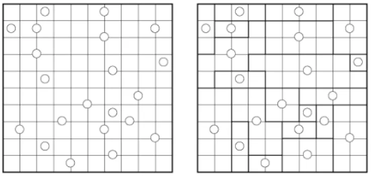
Spiral Galaxies (also called Tentai Show) is a one-player game, described as follows by the Help of its Linux version: “You have a rectangular grid contain-ing a number of dots. Your aim is to draw edges along the grid lines which divide the rectangle into regions in such a way that every region is 180◦
rotationally symmetric, and contains exactly one dot which is located at its centre of sym-metry”. Similarly to many other such puzzles (e.g., Sokoban, Sudoku), apart from being a discrete pastime in boring meetings, it is also a nice combinato-rial and algorithmic problem that one might try to solve computationally. This trend has been developed, among others, by Demaine; see for instance [1], where a survey over hardness results in games is given. For a more general introduction into combinatorial games, we also refer to the book by Hearn and Demaine [6]). Apart from the beauty (and fun!) aspect of such a study, this work is motivated by the fact that while small to medium-size instances of Spiral Galaxies are still fun to solve, larger problems become just too hard, which is frustrating for many players... and might even lead to fits of rage (something you may want to avoid in boring meetings). Hence, an automatic solver for Spiral Galaxies is highly desirable for these cases. In this paper, we thus visit the algorithmic universe of Spiral Galaxies, by providing a series of exact (thus exponential, Spiral Galaxies being NP-hard [5]) algorithms for solving the problem. In particular, we show two fixed-parameter algorithms: one for which the parame-ter is the number of dots (i.e., of galaxies) of the input instance for a constrained version of Spiral Galaxies (where galaxies must be rectangles), and one where the number of “galaxy corners” in a solution is the parameter.
A Formal Problem Definition. We formalize the problem as follows. We have a two-dimensional universe U , where each field in U is described by the coordinate (i, j), where i = 1, . . . , N and j = 1, . . . , M for some N, M ∈ N. We call two
Fig. 1.Two screenshots of a single Spiral Galaxies scenario. Left: the field of squares U with the circular galaxy centers. Right: the corresponding solution. For example, b(1, 1) = g ∈ G, where L(g) = (2, 1). Similarly, b(1, 5) = g′∈ G, where L(g′) = (1, 6.5).
fields (i, j) and (i′
, j′ ) adjacent if |i − i′ | = 1 and j − j′ = 0 or if |j − j′ | = 1 and i − i′
= 0, that is, a field is adjacent to the four fields that are directly left, right, above, and below this field. Let n := |U | be the number of fields. We furthermore are given a set G of k galaxies (’dots’ in the description) along with the location L : G → {1, 1.5, 2, 2.5, . . . , N } × {1, 1.5, 2, 2.5, . . . , M }. We use the noninteger values to denote the case in which a galaxy center is located either between two rows or columns. A galaxy center with noninteger coordinates is adjacent to all fields that can be obtained by rounding its location values. For a galaxy g ∈ G, we use L1(g) to denote the row coordinate of the center of g, and L2(g) to denote
its column coordinate. This is the input of Spiral Galaxies.
There are two natural ways of encoding this input. One is to present each field and each possible galaxy location as a position in a bit string of length Θ(n). Another way is to list the positions of the galaxy centers and the dimensions of the universe. This representation has size Θ(k · log(n)) which is smaller than the first representation if k ≪ n/ log n. Hence, for our exact algorithms we assume that the input length is Θ(n) and for our fixed-parameter algorithms (which assume that k is small) we assume that the input length is Θ(k · log(n)).
A solution to Spiral Galaxies is given by assigning each field of U to some galaxy g. We describe this using the function b : U → G. Before defining the properties of a solution, we give some further definitions. An area A is a subset of U . An area is called connected, if between each field (i, j) ∈ A and (i′
, j′
) ∈ A there exists a path of adjacent fields that belong to A. Two areas A and B are
adjacent if there are two fields α ∈ A and β ∈ B that are adjacent.
In order to be a valid solution, b has to satisfy the following conditions: – rotational symmetry, that is, if b(i, j) = g then b(i′
, j′
) = g, where i′
= 2 · (L1(g) − i) + i and j′ = 2 · (L2(g) − j) + j,
– connectivity, that is, {u ∈ U | b(u) = g} is a connected area, and – hole-freeness, that is, if there is some set G′
of galaxies that is only adjacent to galaxies in G′
∪ {g} for some galaxy g, then at least one element in G′
is at the limit of U .
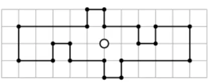
Fig. 2.A galaxy with its corners marked as black dots.
We call (i′
, j′
) ∈ U the g-twin of (i, j). The notation is displayed in the screenshot in Fig. 1. The hole-freeness property is not explicitly demanded by the original problem definition. However, we have not encountered any real-world instance in which some galaxies completely contain other galaxies. Hence, we study the more restricted variant presented here. We believe that our algorithms can, with some technical overhead, be adapted to work for Spiral Galaxies without the hole-freeness property. Note that our definition of a valid solution does not specify that L(g) is inside the galaxy. This property is, however, already guaranteed by the other properties of the solution.
Lemma 1. A nonempty area that is connected, hole-free and symmetric with respect to a location L(g) contains all fields that are adjacent to L(g).
Proof. If the area is a rectangle or shaped like a cross, then the claim holds trivially. Otherwise, assume without loss of generality, that the area contains a field f1which is at least as high as L(g) and to the left of L(g). By the symmetry
property the area, also contains a field f2 that is at most as high as L(g) and
to the right of L(g). Since the area is connected, the two fields are connected by a path of other fields of the area. For each field of this path, its g-twin, however, also belongs to g. Consequently, there are two paths from f1 to f2
that enclose L(g). Since the area is hole-free, this implies that all fields that are adjacent to L(g) belong to the area. ⊓⊔ A corner of an area A is a pair of noninteger coordinates (y, x) such that either one or three of the four neighboring fields (⌈y⌉, ⌈x⌉), (⌈y⌉, ⌊x⌋), (⌊y⌋, ⌈x⌉), and (⌊y⌋, ⌊x⌋) belongs to A (see Fig. 2).
In this paper we present exact algorithms for Spiral Galaxies. In particu-lar, we provide two fixed-parameter algorithms. Note that a problem with input size n is said to be fixed-parameter tractable with respect to a parameter k if it can be solved in f (k) · poly(n) time, where f is a computable function only depending on k. For an introduction to parameterized algorithmics refer to [2].
2
A Nebula of Exact Algorithms
We first provide two exact exponential-time algorithms [4] for solving Spiral Galaxies in the most general case. Though the running times of the two al-gorithms presented here are quite similar, we mention both since they rely on two different viewpoints of the problem. We then focus on the case where any
solution of Spiral Galaxies contains only rectangular galaxies and provide a fixed-parameter algorithm for the parameter number k of galaxies.
Theorem 1. Spiral Galaxiescan be solved in 4N Mpoly(N M ) time. Proof. Given an instance of Spiral Galaxies, any solution can be interpreted as a two-dimensional map, where each galaxy g (and the fields it contains) is a region, and where two distinct regions are adjacent when they contain adjacent fields. The famous four color theorem (see e.g., [8]) tells us that such a map can be colored with at most four colors. The exact algorithm that follows from the above argument can be described easily as follows: generate every possible four-coloring CU of the fields of U ; for each such CU, check whether (a) each
connected set of fields of the same color contains a unique galaxy center, and if so, whether (b) it is a valid galaxy, i.e., it satisfies the symmetry condition and is hole-free. If this is the case, a solution has been found. If no coloring satisfies the two conditions (a) and (b), we have an instance without solution. The running time of the algorithm is straightforward: there are 4 colors and |U | = N M fields to color. Hence the total number of colorings is 4N M; besides,
for any given coloring CU, checking whether conditions (a) and (b) hold can be
done in poly(N M ) time. ⊓⊔
The time complexity can actually be slightly improved as shown in the following. Theorem 2. Spiral Galaxiescan be solved in 24N +MN M poly(N M ) time.
Proof. Take any solution to Spiral Galaxies, and consider two adjacent fields b and b′
. They can be adjacent either horizontally or vertically. If b and b′
belong to distinct galaxies, say g and g′
, we will say there exists a border between them; otherwise, the border does not exist. The algorithm is thus the following: generate all possibilities for borders between adjacent fields (i.e., existence or nonexistence) in U . For each such possibility, compute the maximal connected areas and check whether conditions (a) and (b) from proof of Theorem 1 hold. If this is the case, a solution has been found. If none of the tested possibilities yields a solution, we are in presence of a no-instance. The running time for this algorithm is thus 2nfpoly(N M ), where nf is the number of neighboring fields
in U . The neighboring fields amount to (N − 1)M vertical ones, and (M − 1)N horizontal ones; thus nf = 2N M − N − M , which yields the claimed time
complexity. ⊓⊔
Let Rectangular Spiral Galaxies denote the constrained version of Spi-ral Galaxieswhere a solution may contain only rectangular galaxies. We have the following result.
Theorem 3. Rectangular Spiral Galaxiescan be solved ink!·poly(k log(n))
time.
Proof. The idea here is to guess iteratively, for a free field f (that is, a field not yet belonging to a galaxy), to which galaxy g it belongs, and to branch
on all possible solutions. Any galaxy must have a rectangular shape, thus we choose at each step a free field f which appears as one of the four corners of the galaxy g it will belong to. If such an f exists, knowing f and the center of g is enough to completely determine the shape of g. Now it is easy to see that such a field f always exists: consider for instance, at each iteration, the topmost among all leftmost free fields. The time complexity is straightforward, since at each iteration 1 ≤ i ≤ k, k − i + 1 galaxies centers remain available, and thus we need to branch into k − i + 1 possible cases. Each time a galaxy center is chosen for a field f , computing the dimensions of the rectangle representing the galaxy g that contains f can be performed in O(log(n)) time by subtracting the coordinates of f from L(g) and multiplying the result by two. Note that a free field as described above is always adjacent to one of the four corners of a previously computed galaxy corner, so a free field can be found in poly(k · log(n)) time. Finally, we need to check whether all the rectangles are disjoint, which can be also performed in this running time. Altogether, we obtain the claimed running
time. ⊓⊔
3
An Algorithm for Solutions with Few Corners
It is relatively straightforward to decide in nf(ℓ) time whether there is a
solu-tion with ℓ corners: Guess the exact posisolu-tion and orientasolu-tion of each corner, then connect the corners accordingly and finally check whether this gives a so-lution. The running time follows from the fact that for each corner we have to consider poly(n) choices and that all steps after the guessing can be easily performed in polynomial time.
We now describe an algorithm that can find solutions with at most ℓ corners in f (ℓ) · poly(log(n)) time. The outline of the algorithm is as follows. First, we show how to represent each spiral galaxy as a tiling of O(ℓ) rectangles. Then, we present an integer linear program (ILP) with f (ℓ) many variables which, using a known result on the running time of bounded variable ILPs [7] implies the claimed running time.
Consider any galaxy. Our aim is to represent the galaxy as a tiling of few rectangles. The first step is to divide the galaxy into three parts which will allow us to naturally capture the symmetry condition when defining the rectangle tiling. While doing so, we aim to keep the number of corners low.
Lemma 2. The fields of every galaxyg with ℓ corners can be three-colored with
at most three colors black, red, and blue such that
– ifL(g) has integer coordinates, then the field containing L(g) is black,
oth-erwise no fields are black,
– the red area has at mostℓ + 2 corners, – theg-twin of every red field is blue.
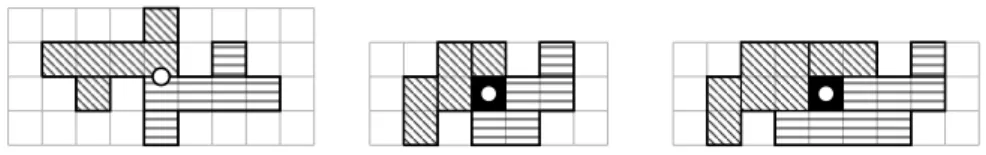
Proof. Let L(g) = (y, x) be the location of the galaxy center. We discuss only the cases in which y is noninteger (the case in which x is noninteger is symmetrical), or in which both x and y are integers (see Fig. 3).
Fig. 3. Examples of some galaxies and the coloring as provided by the algorithm in the proof of Lemma 2 (herein, the red fields are hatched diagonally and the blue fields horizontally). Left: L(g) has noninteger coordinates, middle: L(g) is a separator, right: L(g) has 8 neighbors.
If y is noninteger, then color (⌈y⌉, ⌈x⌉) red. Then check whether there is an uncolored field that belongs to the galaxy and is to the left or to the right of a red field. If this is the case, color it also red. When there is no such field, then note that the row of red fields is a separator of the galaxy. Color the g-twins of this line of red fields (which is the line below) blue. Now color all uncolored fields that can reach blue fields only via red fields with red and all other fields blue. The resulting coloring clearly fulfills the first and the last condition of the lemma. It remains to show the number of corners. At most ℓ/2 corners of the red area are also corners in g. In addition, there are at most two corners between red and blue fields (recall that the separator is a straight line of fields). Since g has at least four corners, the number of corners in the red fields is at most ℓ/2 + 2 ≤ ℓ. If y is integer, then color the field that contains y black. If the galaxy contains no further fields, then the lemma holds. Otherwise, distinguish two further cases.
Case 1: Removing the center from the galaxy cuts the area in at least two connected components. In this case, pick one of these components, color it red and color the fields of its g-twins blue. Then pick, if it exists, another uncolored connected component and color it red and its g-twins blue. No further uncol-ored connected components exist. The red connected components has again at most ℓ/2 corners that are corners in g. Furthermore, there are at most four cor-ners between red fields and the black field. Hence, the number of corcor-ners in the areas defined by the red fields is at most ℓ/2 + 4 ≤ ℓ + 2.
Case 2: Otherwise.In this case, the galaxy center has eight neighbors. Color the field to the left of the center red and call it the current field. While the current field has a left neighbor that is part of g, color this field red and make it the current field. Next, make the field to the top-left of the galaxy the current field and color it red. Now, while the current field has a right neighbor that belongs to g, color it red and make it the current field. Now, the red fields are a separator. Color all fields that can reach the center only via red fields also with red. After this, color all g-twins of the red fields blue.
Again, the area defined by the red fields has at most ℓ/2 corners that are corners in g plus four corners on the border to the blue or black fields. The overall number of corners is thus at most ℓ/2 + 4 ≤ ℓ + 2. ⊓⊔ In order to formulate the ILP we will model each galaxy as a union of rect-angles. The following lemma is a straightforward corollary of [3, Theorem 1].
Lemma 3. An orthogonal polygon with ℓ corners can be partitioned into at
mostℓ nonoverlapping rectangles.
Definition 1. Arectangle representation of a galaxy g is a set of rectangles Rg= {R1, R2, . . . , Rq} such that:
– the union of allRi is exactly g, – Ri andRj do not overlap if i 6= j,
– for eachRi, there is exactly one rectangleRj∈ Rgsuch that the four corners
ofRj are exactly theg-twins of the four corners of Ri.
For a galaxy representation, we use s(Ri) to denote the rectangle that is
symmetric to Ri.
Lemma 4. A galaxy g with at most ℓ corners has a rectangle representation
with O(ℓ) rectangles.
Proof. By Lemma 2 we can partition g into three areas that have O(ℓ) corners altogether. Now, for the red part we choose some partition into O(ℓ) rectangles which exists by Lemma 3. For the blue part choose the symmetric (with respect to L(g)) partition into rectangles. The black part, if it exists, is a rectangle so add the corresponding rectangle if it exists. Clearly, the union of the rectangles is g, the rectangles do not overlap and, by the choice of the partition of the blue part, there is for each red rectangle Ri a symmetric blue counterpart Rj. The
black rectangle R, if it exists, consists just of one field whose center is L(g), so the corners of R are symmetric to themselves. ⊓⊔ We now use the rectangle representation to fix the main structure of a putative solution. A layout of a solution is a structure consisting of the following parts:
– For each galaxy g, we fix a set of rectangle identifiers Rg
1, . . . , R g
q, q = O(ℓ).
– For each rectangle Rgi, we fix s(Rig) (note that if L(g) has integer coordinates, Rgi = s(R
g
i) is possible).
– For each pair of rectangles Rg
i and R g′
j , we fix whether R g
i is above, below,
to the left, or to the right of Rgj′ (at least one of the four must be the case).
– For each pair of rectangles Rg
i and R g′
j , we fix whether they are adjacent or
not, and if this is the case, we fix the “extent” of the adjacency. For example, if Rgi is above R
g′
j , then we fix whether the left side of R g′
j is at least as far
to the left as the left side of Rigor not, and similarly, whether the right side
of Rgj′ is at least as far to the right as R g i or not.
– For each rectangle, we fix whether it is adjacent to the left, right, top, or bottom limit of the universe.
Clearly, the number of layouts is bounded by a function of ℓ since the number of rectangles to consider in any solution is O(ℓ). The main structure of the algorithm is now as follows. Try all possible layouts. For each layout, first filter “bad” layouts that do not guarantee that the galaxies are connected, that the
galaxies are hole-free, or that they cover the whole universe. Then, create an ILP with O(ℓ) variables and solve it. If it has a feasible solution, then use this solution to construct a solution of Spiral Galaxies.
We now describe how to filter bad layouts. For each galaxy g, create a graph whose vertices are the rectangles Rgi. Make two vertices adjacent in this graph if
the corresponding rectangles are fixed to be adjacent by the layout. Reject the layout if the resulting graph is not connected for some galaxy.
Now create a graph whose vertices are the galaxies. In this graph, make two galaxies g and g′
adjacent if there is a pair of rectangles Rgi and R g′
j that are
fixed to be adjacent by the layout. Furthermore, add one vertex that represents the limits of U and make it adjacent to each galaxy g that has a rectangle Rgi
that is fixed to be adjacent to the respective limit. Now, reject the layout if there is a galaxy g that is a cut-vertex in this graph, that is, there is a pair of galaxies g′
6= g and g′′
6= g such that all paths between g′
and g′′
contain g. Finally, consider each rectangle Ri of the layout that is adjacent to at least one
other rectangle. Assume without loss of generality, that the bottom fields of Ri
are adjacent to the rectangles Q1 i, . . . , Q
q
i, which are ordered such that
– the left border of Q1i is fixed to be at least as far to the left as the left border of Ri and there is no other rectangle Q
j
i for which this holds,
– the right border of Qqi is fixed to be at least as far to the right as the right border of Ri and there is no other rectangle Q
j
i for which this holds, and
– for i′
> 1, Qi′
i is fixed to be adjacent and to be to the right of Q i′−1 i .
If such an order does not exist, then reject the layout. Otherwise, we build the ILP formulation. We only need to check for feasibility, hence there will be no objective function that we need to maximize.
For each rectangle Ri in the layout, we introduce four variables: x1i, y1i, x2i,
and y2
i, where (y1i, x1i) shall be the top-left field of Ri and (y2i, x2i) shall be the
bottom-right field of Ri. No further variables are introduced and the number of
variables thus is O(ℓ). We now introduce inequality constraints that guarantee that the ILP solution gives a solution to Spiral Galaxies. First, we constrain all coordinates to be in the universe.
∀xji : 1 ≤ x j i ≤ M (1) ∀yji : 1 ≤ y j i ≤ N (2)
The second set of constraints forces all rectangles to be nonempty and guarantees that the coordinate pair (y1
i, x1i) is indeed the top-left field.
∀x1i :x1i − x2i > 0 (3) ∀y1i :y 1 i − y 2 i > 0 (4)
Now we introduce constraints for rectangle pairs to force that the rectangles do not overlap, that adjacencies are preserved as fixed in the layout, and that each galaxy is symmetric. Herein, we describe only the case in which the rectangle Ri
is above Rj, all other cases can be obtained by rotating the universe. First, we
guarantee that the rectangles do not overlap. y2
i − yj1> 0 (5)
If Ri and Rj are fixed to be the corresponding rectangles in the two symmetric
parts of a galaxy g, that is, Ri= s(Rj), then assume without loss of generality,
that the right border of Riis not to the left of the right border of Rj. Then, we
add the following constraints.
2 · L2(g) − x1i − x2j = 0 (6) 2 · L1(g) − yi1− yj2= 0 (7) 2 · L2(g) − x2i − x 1 j = 0 (8) 2 · L1(g) − yi2− yj1= 0 (9)
Now, we add the constraints concerning adjacent rectangles. If Ri and Rj are
fixed to be adjacent, then, since Ri is above Rj, we add the constraint
y2
i − yj1= 1. (10)
If we fix the left border of Rj to be at least as far to the left as the left border
of Ri, then we add the constraint
x1i − x 1
j ≤ 0. (11)
We add similar constraints for the right borders of Ri and Rj (according to
whether or not we have fixed Ri to extend further to the right than Rj).
Finally, we add the following constraints for the rectangles that are adjacent to the limit of the universe.
y1
i = 1 if Riis adjacent to the top limit of U (12)
yi2= N if Ri is adjacent to the bottom limit of U (13)
x1i = 1 if Ri is adjacent to the left limit of U (14)
x2i = M if Ri is adjacent to the right limit of U (15)
Lemma 5. If the ILP as constructed above has a feasible solution, then the Spiral Galaxiesinstance is a yes-instance.
Proof. First, we show that the rectangles that are fixed to make up a galaxy g create an area that fulfills the properties of a galaxy. By the filtering step and by Constraint 10, the area created by the rectangles is connected. Furthermore, every field in this area is contained in a rectangle. By Constraints 6–9 there is a rectangle whose corners are g-twins of the rectangle containing this point. Hence, the g-twin of the each field is also contained in g. Now, by the filtering step before the ILP construction, the galaxy is also hole-free and therefore it fulfills all properties of a galaxy.
It remains to show the global property that the rectangles form a partition of the universe. By Constraint 5, the rectangles do not overlap, so it remains to show that the rectangles cover the universe. Assume that this is not the case. Then there is some field not covered by any rectangle but adjacent to some rectangle Ri. Assume without loss of generality that this field is below Ri.
Clearly, Riis not fixed to be adjacent to the bottom border by the layout. By the
filtering step, the field Rithus has at least one neighboring rectangle that is fixed
to be below Ri and extend further at least as far to the left than Ri. Similarly,
such a rectangle exists for the right border of Ri. Furthermore, between these
two rectangles the filtering step guarantees that there is a chain of horizontally adjacent rectangles that are below Ri and adjacent to Ri. Hence, every field
below Ri is covered by some rectangle. ⊓⊔
The converse of the above statement is also true in the sense, that if there is a solution to Spiral Galaxies, then there is one layout which passes the filtering and whose constructed ILP has a feasible solution. The existence of this layout is guaranteed by Lemma 3 plus the fact that the filtering step does not remove this layout. The feasible ILP solution is then obtained by simply plugging in the coordinates of the rectangles. Altogether we thus obtain the following.
Theorem 4. Spiral Galaxiesparameterized by the numberℓ of corners of a
solution is fixed-parameter tractable.
Proof. The correctness follows from Lemma 5 and the discussion above. It re-mains to show the running time. The number of layouts to consider is bounded by a function in ℓ since the number of galaxies is O(ℓ) and the number of rectan-gles that we need to consider for each galaxy is also O(ℓ). Hence, the number of objects for which all different possibilities of “applying some fix” only depends on ℓ. Therefore, the number of ILPs to solve is also only a function of ℓ. Since each ILP has O(ℓ) variables and O(poly(ℓ)) many constraints it can be solved in f (ℓ) · poly(log(n)) time [7]. All other steps can be performed in polynomial
time. ⊓⊔
4
Outlook
We conclude with two open problems. First, is Rectangular Spiral Galax-iessolvable in polynomial time? Second, is Spiral Galaxies fixed-parameter tractable with respect to the number k of galaxies? A natural approach to show fixed-parameter tractability for k would be to show that the solution has only f (k) corners. Indeed, we tried to show that this is the case. However, even for four galaxies only, this is not true.
Theorem 5. For every ℓ ∈ N, there are yes-instances of Spiral Galaxies
with four galaxies such that every solution has more thanℓ corners.
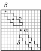
Proof. Let x > ℓ + 2 and consider the following instance with N = M = 2x + 1 and four galaxies α, β, γ, δ. In the instance, α will be very large, γ and δ will
α β
γ
δ
Fig. 4.An instance of Spiral Galaxies with four galaxies and many corners.
be small, and β will be tiny. To denote the positioning of the centers of the small galaxies, we introduce another variable y which is some even integer such that ℓ ≤ y < x. The four galaxy centers are as follows.
– L(α) = (x + 1, x + 1), – L(β) = (1, 2),
– L(γ) = ((y + 3)/2, y/2 + 5/2), and – L(δ) = (2x + 1 − y/2, 2x − y/2).
A sketch of the instance and of a solution for one set of values of x and y is given in Fig. 4.
First, observe that by the choice of y, the galaxies β and γ live in the upper-left quadrant, that is, the set of fields (i, j) with i, j ≤ x+ 1, and galaxy δ lives in the lower-right quadrant. Therefore, all α-twins of fields of β and γ must belong to δ. Hence, the shape of δ is a union of the shapes of β and γ. Further, galaxy β has its center on the last row of U , so it must be flat (have height one) and, since its center is on the second column, it can be either a galaxy containing just the center or a flat galaxy of width three.
We now show that the solution must essentially look like the one shown in Fig. 4. The center of β does not belong to α, so its α-twin which is (2x + 1, 2x), belongs to δ. But then the δ-twin of (2x + 1, 2x) belongs to δ as well. This field is (2x − y + 1, 2x − y). Now, the α-twin of this field is (y + 1, y + 2) and it is again not in galaxy α, so it must be in galaxy γ (recall that β is flat). Now the main difference between γ and δ that creates the many corners is the following. The height difference for γ-twins is odd since its center sits at noninteger coordinates. The height difference for δ-twins, however, is even since δ’s center sits at integer coordinates. Moreover, the height of γ is exactly y since it cannot reach fields above (y + 1, y + 2) (their α-twins are unreachable for δ). Therefore, galaxy γ has at least one field in each row from row y + 1 until row 2. Similarly, galaxy δ has at least one field in each row from row 1 until row y + 1. Note that for galaxy δ the formula (i + 1, i) defines a straight diagonal line between the three fields that are already assumed to be in δ. We now show a statement which implies that the fields of δ must be close to this main diagonal.
Claim.For 1 < i ≤ y + 1 and 1 ≤ j < 2x − i, if (2x + 1 − i, 2x − i − j) belongs to δ, then (2x + 2 − i, 2x + 1 − i − j) belongs to δ.
If (2x + 1 − i, 2x − i − j) belongs to δ, then its α-twin (i + 2, i + 3 + j) belongs to γ (since i > 1 it cannot belong to β). Therefore, the γ-twin of this field also
belongs to γ. This field is (y + 1 − i, y + 2 − i − j). Again, the α-twin of this field belongs to δ. This field is (2x − y + i, 2x − 1 − y + i + j). Finally, the δ-twin of this field belongs to δ. This field is (2x + 2 − i, 2x + 1 − i + j) which proves the claim.
Now, we know that (2x + 1, 2x + 2) cannot belong to δ as it is outside of the universe. Hence, the maximum deviation of δ from the main diagonal to the right is one, which implies that the maximum deviation of δ from the main diagonal to the left is also one. We also know that in row 2x − y, the field that is on the main diagonal belongs to δ. By the above claim the complete main diagonal thus also belongs to δ. Since the galaxy is connected, this implies that either in row 2x − y or in row 2x − y + 1 the right or left neighbor of the main diagonal also belongs to δ. Again by the above claim this implies that either the left or the right neighbor of the main diagonal is part of δ for all rows i ≥ 2x − y + 1. By the symmetry of the galaxy we then obtain that the left and right neighbor of the main diagonal have to belong to δ for all rows of δ.
Hence, each of the y + 1 rows of δ, i.e., rows 2x − y to 2x + 1, has two corners. Therefore, the overall number of corners is larger than ℓ. It is easy to verify, that there is indeed for all x and y as chosen above a solution: the galaxy δ is as described, the galaxy β is a flat galaxy with width 3, the galaxy γ is the set of remaining α-twins of the fields that are in δ, and all other fields are in α. ⊓⊔ Currently, we don’t have a conjecture on either of the two questions. We do have a proof that the answer is not 42 but we defer it to a full version of the paper.
Acknowledgments. We thank the anonymous referees of FUN 2014 for several comments improving the presentation of this paper.
References
[1] E. D. Demaine. Playing games with algorithms: Algorithmic combinatorial game theory. In Proc. 26th MFCS, volume 2136 of LNCS, pages 18–32. Springer, 2001. Available at http://arxiv.org/abs/cs.CC/0106019. [2] R. G. Downey and M. R. Fellows. Fundamentals of parameterized complexity.
Undergraduate Texts in Computer Science, Springer-Verlag, 2012.
[3] L. Ferrari, P. Sankar, and J. Sklansky. Minimal rectangular partitions of digitized blobs. Computer vision, graphics, and image processing, 28(1):58– 71, 1984.
[4] F. V. Fomin and D. Kratsch. Exact exponential algorithms. Springer, 2010. [5] E. Friedman. Spiral galaxies puzzles are NP-complete. Available at http:
//www2.stetson.edu/~efriedma/papers/spiral.pdf, 2002.
[6] R. A. Hearn and E. D. Demaine. Games, puzzles, and computation. AK Peters, Limited, 2009.
[7] R. Kannan. Minkowski’s convex body theorem and integer programming.
Mathematics of operations research, 12(3):415–440, 1987.
[8] N. Robertson, D. P. Sanders, P. D. Seymour, and R. Thomas. The four-colour theorem. J. Comb. Theory, Ser. B, 70(1):2–44, 1997.