DESIGN TROTTER: Inter-Function Cycle Distribution Step

HAL Id: hal-00008493

https://hal.archives-ouvertes.fr/hal-00008493

HAL is a multi-disciplinary open access archive for the deposit and dissemination of sci-entific research documents, whether they are pub-lished or not. The documents may come from teaching and research institutions in France or abroad, or from public or private research centers.

L’archive ouverte pluridisciplinaire HAL, est destinée au dépôt et à la diffusion de documents scientifiques de niveau recherche, publiés ou non, émanant des établissements d’enseignement et de recherche français ou étrangers, des laboratoires publics ou privés.

DESIGN TROTTER: Inter-Function Cycle Distribution

Step

Thierry Gourdeaux, Jean-Philippe Diguet, Jean-Luc Philippe

To cite this version:

Thierry Gourdeaux, Jean-Philippe Diguet, Jean-Luc Philippe. DESIGN TROTTER: Inter-Function Cycle Distribution Step. Real-Time Systems, 2003, Paris, France. �hal-00008493�

DESIGN TROTTER:

Inter-Function Cycle Distribution Step

Thierry Gourdeaux, Jean-Philippe Diguet, Jean-Luc Philippe Université de Bretagne Sud, LESTER Lab., BP 92116, 56321 Lorient Cedex

tel: 0/33 2 97 87 45 60 Fax: 0/33 2 97 87 45 00

e-mail: firstname.name@univ-ubs.fr http://lester.univ-ubs.fr

ABSTRACT

This work is located in the domain of System On Chip design and specifically addresses the question of HW/SW parallelism allocation and scheduling at a system level. This paper describes the inter-function (or inter-task) estimation step within our system-level design framework. Given resource/delay trade-off curves for each function (i.e. functional block) of a complex application we propose a genetic-based method to the distribute time ratio over the set of functions in order to respect the time constraints while favoring intra and inter-function resource sharing. The aim of this task is to provide a global approach of the system in order to converge towards a promising HW/SW target architecture.

KEY WORDS

Partitionning, Scheduling, SystemLevel, Genetic Algorithm

CONTACT

I)

INTRODUCTION

In order to face the challenge of high performance/area and performance/power ratios (PAR, PPR), the design of embedded systems is turning into the optimized selection of tuned and heterogeneous systems on chip (SOC). The objective is to meet the best fitting, mainly in terms of power, area, performance and QoS, between the application(s) and the chip components within a time window matching the market requirements. The main issue in this domain is to cope with the trade-off between the exploration of a huge design space and the accuracy of solution evaluations. Generally this question is handled through a refining process which consists in reducing the search space while increasing the estimation time with more accurate architectural models.

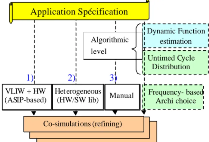
Then three kinds of approaches are proposed regarding the design space exploration (see Figure 1). The first one includes library-based HW/SW partitioning frameworks that automatically perform an implementation choice for each task (real-time systems) or functions (control data-flow) within a reduced set of hardware or software pre-characterized solutions [1,2,3]. The second solution consists in tuning a generic predefined architecture with the objective of finding the optimal parameters. In [4], the authors use the dependencies between parameters to efficiently prune the design space. The target architecture is based on three components to be parameterized: a VLIW processor, a memory hierarchy and a HW accelerator. Pertinent design space decomposition is detailed in [5] where moreover the choice of parameters is driven by the clustering of valid and Pareto-optimal sets of previously evaluated components. A third class of methods stresses primarily the simulation and model aspects while considering a manual application partitioning. For instance, Spade [6] is a modeling and simulation environment that handles several abstraction levels. The architecture units workloads are manually analyzed by the designer in order to perform HW/SW partitioning and iteratively refine the architecture. VCC [7] from Cadence is help for the system definition and functional validation but with serious restrictions regarding the limited set of architectural models for temporal simulation.

All these solutions are located after a key point, which is the parallelism distribution within, and inter the different functions composing the application. A function can have the granularity of a task if an embedded RTOS is considered or the sense of a functional block within a standard description (for instance DCT, motion estimation blocks). We have addressed the inter-function issues in two different ways. In [8] the question is solved with a HW/SW codesign framework based on a static and preemptive scheduling, which enable to handle periodic and multi-cadences tasks. In this paper, the approach is different, the application is modeled as a coarse grain data-flow graph where each node represents a functional block including it's own control. It has been proved [9] that algorithmic transformations and parallelism management before architecture assignment can provide significant gains especially in terms of power within the domain of data-transfers in multimedia applications. Actually, regarding the global optimization of the function-level parallelism, a couple of decisions have a great influence on the quality of the final solution (i.e. PPR, PAR). These decisions are:

i) the parallelism to be exploited within a function : from a fully parallel to a restricted sequential implementation ii) the choice of parallel execution between the different functions : the starting dates of the functions (i.e. a coarse grain scheduling)

If we refer to the metaflow described in [9], these aspects are intra an inter-task concurrency management. So, we propose an approach which is based on two main steps: the intra-function parallelism estimation for various cycle budget (ideally from the critical path to a sequential execution) and an inter-function parallelism management. This paper focuses on the second step, currently the resources considered are data-transfers and processing operations. The first step aspects are described in [10][11].

As explained in Figure 1, our strategy starts with a dynamic estimation of each application function. This estimation is based on a architecture definition whose the accuracy depends on the designer description. Each cycle budget ∆T from the dynamic estimation provides the inter-function step with a scheduling profile [0-∆T] for each data-transfer and processing resource. Then, a first part of the inter-function step consists in a distribution of cycles over the set of functions (Fi) in order to balance resource use. In a second part, a reduced set of solutions is saved and a second cycle distribution step is launched with more accurate information about the cycle values and instruction dependencies. Namely, we operate a technology mapping. Note that depending on the target

architecture different frequencies can be handled, the term codesign is not really adapted since each frequency can be associated with a HW or SW areas from an heterogeneous set: {SW1(F1)..SWN(FN) ; HW1(F'1) ..HWM(F'M)}. In

this paper we focus the inter-function cycle distribution based on a genetic algorithm. For simplicity without loss of generality we use a reduced set of two frequencies associated respectively to HW and SW parts. The method aspects are detailed in the next section.

Figure 1: Design Space exploration approaches Figure 2: Refining stages

I.1)

Problem Formulation

The general optimization problem we address is: "Given a set of functions described as a task graph, given a set of data transfer and processing resources, given a set of scheduling profiles for each task corresponding to various cycle budgets, given a set of available cycle clocks corresponding to various HW or SW area on the target SOC and given a global time constraint, assign a cycle budget and a frequency to each function and decide the starting date of the scheduling of each function in order to minimize resource."

I.2)

Key contribution

Conjoint approach for inter and intra function (or task) parallelism management for resource use optimization.

II)

REFINING STAGES

The tool, under development, operates stage by stage by proposing for each of them a set of solutions in order to gradually converge towards an optimized architecture. Each decision reduces the number of solutions and provides a set of inputs to the optimization next stage. These stages are presented in Figure 2.

II.1)

System Exploration Stage

At this level, we use abstract cycles since the target architecture is not yet defined. The aim is explore resource parallelism to me mapped in the subsequent flow steps.

II.2)

"Codesign" Stage

At this level, the aim is to respect a time constraint ∆T while minimizing resource and favoring resource sharing within and inter functions. However, the common time unit is an abstract cycle, so we need to map cycles into time. Considering a heterogeneous architecture and power minimization, we use the period of different clocks. Namely, each clock period corresponds to a SOC area within which resource sharing is possible. In addition, note that constraints on resource availability can be introduced in order to model a SOC area associated to a processor core. Thereafter, we'll see they could be integrated in the design flow. The solutions provided at this stage give a qualitative approach by specifying the target of the resource (processor, coprocessor, and accelerator) and

Co-simulations (refining) 1) 2) 3) 4) Algorithmic level VLIW + HW (ASIP-based) Het erogeneous (HW/SW lib) Manual Frequency- based Archi choice Untimed Cycle Distribution Dynamic Function estimation Application Spécification System exploration Codesign Codesign + communications Logic Synthesis

quantitative by giving the minimal time of execution, the selected frequencies and especially the number of resources used. This paper addresses this second stage.

II.3)

"Codesign + Communications" Stage

Given a set of promising solutions from the second stage, we can perform the last exploration step while considering communications between functions. In the previous step only data-transfers were considered, however we need bus and buffer accurate models to finally select the final solution. This part is currently studied and won't be developed in this paper.

III)

PROBLEM FORMULATION

III.1) Algorithm Input Data

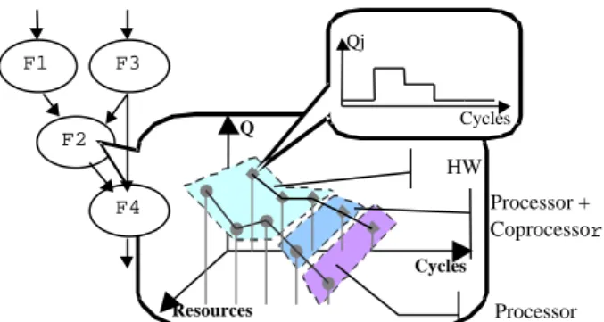
The algorithm input is a function graph called subsequently SLDFG (System Level Data Flow Graph). At each function is associated a trade-off curve which represents, for a given cycle budget, the amount of required resources. Each point of the trade-off curve provides a data quadruplet [10][11], which specifies (see Figure 3): - the cycle budget

- ∀j ∈ Set(resources) the quantity Qj of resource j

- The SOC component target (SW core, SW core + Coprocessor or HW) - Resource scheduling profile

Note that a function can't operate on several kind of targets simultaneously, e.g. the resource sharing between functions is only possible if functions belong to the same frequency area. Moreover, available frequencies required for the "codesign" stages, are specified by the designer.

Figure 3: SLDFG and data associated

III.2) Paths definition

To simplify exploration and scheduling, the SLDFG is converted into an array of data paths. Figure 4 is the array representation of the SLDFG in Figure 3. We observe three paths P1 {F1,F2,F4}, P2 {F3,F2,F4} and P3 {F3,F4}. Each path is characterized by a scheduling priority order. The SLDFG is traveled with a depth first search algorithm in order to solve function dependencies while taking into account the path priority order. Thus, the mobility of functions, which belong to weak priority paths, is constrained by high priority paths. We'll see later how, for a given solution, the path priority is initially

randomly generated. Figure 4: Paths array

F2 Q Cycles Resources _Processor HW Cycles Qj F1 F4 F3 Processor + Coprocessor

P1

P2

P3

F1

F3

F3

F2

F2

F4

F4

F4

III.3) Time distribution within a path

Time constraints are also assigned to functions through a priority-based mechanism. Each path Pi must respect a delay constraint ∆Ti, in each path a time ratio D(Fk)=∆Ti.P(i,k)/N is allocated to each function k, where P(i,k) is the priority of the function k, such as for each path i : ∑kP(i,k)= N. The parameter N enables the designer to tune the size of the solution space. Note that if a function k belongs to a previously scheduled path i', then its delay is already fixed (i.e. this is a scheduling constraint for the path i)

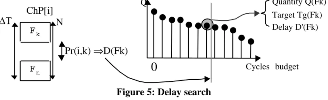
In the "codesign" stage, this priority Pr(i,Fk) is converted into a delay D(Fk) allocated to the application. Regarding the function time ratio, the algorithm searches in the trade-off curve, the solution with the closest delay

D'(Fk) lower than D(Fk) (Fig.5). The cycles to time conversion is computed by choosing one of the available

SOC operation frequencies (i.e. a target Tg(Fk)). We will see in the next section how these frequencies are selected or fixed by the designer. The quantity Mi(Fk)= D'(Fk) - D(Fk) is the intrinsic mobility of the function k.

ChP[i] F_k F_n Pr(i,k) ⇒D(Fk) N ∆T Quantity Q(Fk) Target Tg(Fk) Delay D'(Fk) Cycles budget Q

0

Figure 5: Delay search

III.4) Mobility due to path common functions

A function can belong to several paths. The coarse grain scheduling must then favor resource-reuse within each target while respecting precedence constraints. A given node in the SLDFG is first characterized by its intrinsic mobility, which can be used in order to choose a scheduling date which optimized resource reuse. However, the starting date and the allocated delay of a given node also depend on previously scheduled nodes. In figure 4 for instance, if the path P1 is firstly scheduled then two cases happen for the scheduling of the function F3. First, in

order to respect delays we set: D'(F2) = Min{D'(p1,F2); D'(p2,F2)}.

Then if D'(p1,F1) > D'(p2,F3) then mobility of F3 is : M(F3) = Mi(F3) + (D'(F1)-D'(F3)) else if D'(p1,F1) <

D'(p2,F3) : M(F3)= Mi(F3).

Figure 12 gives a graphical view of scheduling with both mobilities and scheduling profiles. For example, the functions 1, 2, 3 are concurrent to functions 9, 10, 11 and share several resources. The zoom shows the global mobility, which is the summation of the extrinsic mobility (ALAP-ASAP) and the intrinsic mobility (difference between date computed from priority and the selected implementation). Depending on the scheduling profile of F1 and on the optimization strategy (fine or coarse grain, see section 3.6), the mobility of F10 can be exploited in order to optimize resource sharing with F1 (bus, ALU).

III.5) Information Coding

The resource use during the application execution can be seen as a hollow matrix, thus an optimized coding is obtained while only storing the peculiar points.

Q=2 [60..90] Q=1 [10..20] Q=1 [90..110] 10 20 60 90 110 Q

Figure 6: Information coding

Each kind of resources consists in a set of block chained lists. Each block corresponds to a given quantity of resource used during a time period. For instance in Fig.6, one unit is used within the time slots [10..20] and

[90..110] while two units are required within the interval [60..90]. Regarding resource sharing, an additional information is the list of functions using this resource during this period. Moreover each kind of resources can be associated with different frequencies, but resource sharing is possible between functions using the same kind of resource with the same frequency (i.e. on the same target). Figure 7 shows the data structure: each individual is coded as an array that indicates the resource use. Each array cell contains a chained list of frequencies used for this kind of resource, then each node of this chain if a block specifying : the number of resources used, the functions using it and the start and end dates.

R-1 R+1 R Qty=3 Begin=4 End=9 Functions=f1, f3 Qty =1 Begin =10 End =15 Functions = f3 Qty =2 Begin =2 End =12 Functions =f2 Freq 1 Freq f

Figure 7: Resources occupation coding

III.6) Coarse & fine-grain function Scheduling

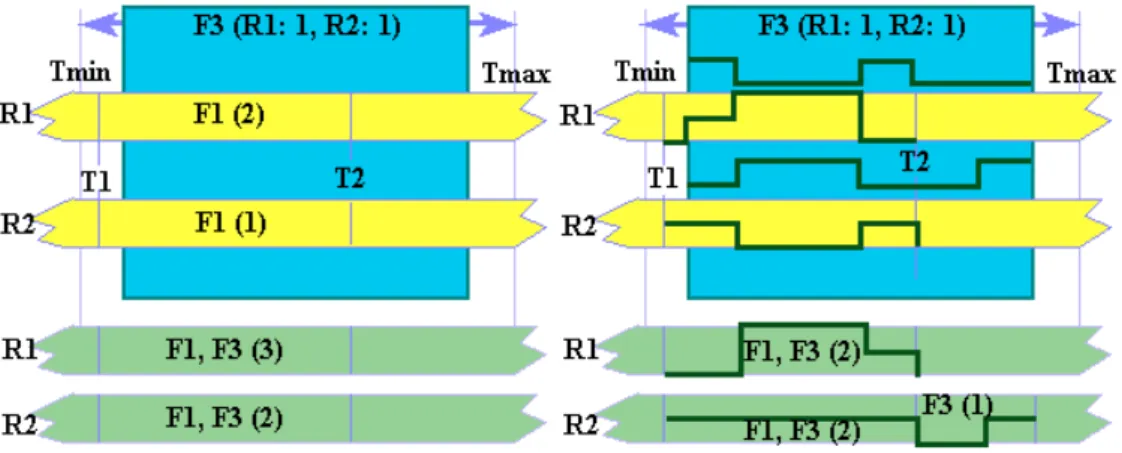
We have implemented two kinds of resource sharing optimizations. The first one, called coarse-grain scheduling, is based on the maximal resource quantities required by each. For instance in Fig.8a, the global mobility of F3 is such as, F3 has to schedule between Tmin and Tmax. In this slot time, F1 uses a maximum of 2 resources of type F1 between T1 and T2 while F3 requires one resource of this type. So the number of ressources allocated equals to 3 during this period. The fine-grain scheduling, explores the scheduling profiles of functions in order to get resource sharing at a cycle level.

Figure 8: Coarse/fine-grain estimation for function insertion

In Figure 8b, the scheduling function F3 does not increase the quantity of resources, since its profile is complementary to F1 profiles R1,R2). On the other hand, in Figure 8a, without precise information, the quantities of F3 resource are added to those required by F1. Thus, the time distribution procedure can be seen as a slide-rules (whose the width is equal to number of cycles allocated to the function) moving from an interval to an other one while seeking the best matching with the occupation profiles of each resource Rj. This is clearly a trade-off between the speed and the optimization degree, which is decided by the designer. For each resource, the designer can either let the algorithm finding the minimum quantity of resources, or specify a maximum quantity not to exceed. For instance, in Figure 8a, the case is not disqualifying if the upper limit of R1 is a least 3.

III.7) Exploration and scheduling method choice

The scheduling problem under time constraint while minimizing resource is known to be NP complete, moreover we address the scheduling of functions characterized by cost/delay trade-off curves, which means in practice a "double-level" scheduling problem. So, an exhaustive search is a non-sense regarding the solution space size, however the characteristics of the search space are the following.

i) Due to the level of abstraction, the graph size is quite reasonable. Actually we focus on a data-flow graph at a system level where a node represents a functional block. So, it means that the graph size is typically lower that a hundred of nodes while the number of implementation solutions for each node is around ten.

ii) There is no obvious "a priori" good solutions, the introduction of hazard has been considered as a necessity like the possibility of getting out local optimal during the exploration.

On one hand, a branch & bound has been firstly considered, but it appeared to be too slow because of be the width of the resulting tree. Moreover, the nature of the problem make the heuristics very difficult to control in an efficient way and it was possible to easily explore different path scheduling priorities. Different other greedy approaches didn't provide good results mainly because of the issue of priority during the scheduling. Finally a genetic method appeared to be an interesting approach to manage isotopic search, to control the solution space explosion and the exploration delay in a very parallel way.

IV)

GENETIC ALGORITHM

Genetic Algorithms (GA) are based on evolutionary models in which the most fitted individuals have more chances to survive. Starting with a population where all individuals have been randomly generated, GA tries, generation after generation, to improve the population average fitness in order to find the best individual, i.e. an optimal solution. In our case, an individual corresponds to the partitioning/scheduling of the application function. GA uses two operators to combine two individuals in order to produce new solutions. These operators are crossover and mutation. The first one mixes two chromosomes to generate a new one (or two), and the second randomly modifies a gene inside a chromosome (i.e. a parameter of a given solution). Quality of solutions and convergence speed depend on population size, mutation and crossover ratio, selection and replacement methods. All these parameters are chosen empirically. Genetic Algorithms have already been used for solving classical scheduling problems in high-level synthesis [12,13] or in job-shop scheduling [14]. The main difficulty is to be able to manage constraints (precedence, allocation etc...) without including a critical verification step between each generation production i.e. to produce individual which represent feasible solutions.

In fact, in order to perform both partitioning and scheduling we have defined an hybrid genetic algorithm. The GA only generates the parameters for each individual (function priority, frequencies…) which conduct to a potential efficient solution (good fitness between constraints (resource, time, consumption, communication)) and the scheduling algorithm (Depth First Scheduling [15]) enables to schedule each function of the application.

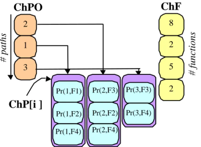
IV.1) Chromosome Encoding

Genes are usually encoded as bit strings. However it would be the detection of aberrant crossover would be inefficient. For this reason, we chose a natural coding. A solution is coded with three kinds of chromosomes. The first one ChPO gives the priority of path proceeding. For instance, in Figure 9 we observe that the proceeding order is {P2,P1,P3}. Thus, the path coded in the first gene is scheduled first and the following paths are then constrained by their predecessors. This coding has been chosen in order to favor critical paths.

The second kind of chromosomes is the components of the array ChP[i], which represent the SLDFG. Each chromosome ChP[i] gene contains Ni genes corresponding to the Ni functions within the path i.

Figure 9: Coding of chromosomes

A gene is a value representing Pr(i,Fk): the ratio of time which has to be allocated to the function k. The third kind of chromosome ChF contains the coding of available frequencies (i.e. target Tg(Fk)), a gene value is an index of the frequency array. The priority-based coding for paths, time allocation and mobility use is very important since it enables to produce few unfeasible solutions (lethal individual: an unfeasible solution is generated when the time ratio allocated to a function is lower than its critical path). Thus we avoid the implementation of a time-consuming procedure to check the solutions validity.

IV.2) Operators

Crossover

The crossover probability usually ranges from 20 to 60% [12]. Thanks to the chosen coding, genes are independent. The uniform crossover is the adopted method. It is a swap of a continuous succession of genes between two randomly selected points. Nevertheless, since the quantity, the content and the meaning of genes varies from a chromosome to another, crossover are only feasible between two same kind of chromosomes ie: ChPO, ChF or ChP[i]. For the last one ChP[i], the crossover are performed between two genes representing the same path (a given value for i) because they must have the same number of genes. Since ChPO contains all the paths only one time, a modified uniform crossover is applied to ovoid doubloons.

Figure 10: Uniform crossover Mutation

The mutation probability typically ranges from 0.1 to 1% [12]. The mutation allows maintaining a relative diversity in population, and thus avoids focusing on a local optimum. As for the crossover operator, a modified mutation is applied to ChPO to insure not having two times the same chromosome.

C1

C2

C1

C2

ChPO

ChF

ChP[i ]

IV.3) Objective Function

The objective functions gives some measure of individual fitness with respect to the population average. It permits to distinguish the best individuals from the worst, and thus to select which solutions will be part and parents of the next population. In a first time we adopt an objective function as used in high-level synthesis [12]. The area is obtained for HW resource technologic libraries. This model will be completed with communication and consumption costs in future work.

Equation 1: Objective function

IV.4) Initial Population

The initial population is randomly generated such as all the individuals created are viable. In order to converge quickly, the initial population is partly generated with the solution set of the preceding phase. At the end, a reduce number of good solutions is provided to the designer who takes the final decision.

V)

EXAMPLE

As example, we use the "biped soccer player" application conjointly developed with the a robotic lab. Many of these functions implement image and signal processing algorithms. Figure 11 gives the SLDFG of the robotic

Table1: Required resources Figure 11: SLDFG and chromosome coding

C is the number of paths

dFc et bFc are respectively the delay

and start cycle of the last function F of the path c

R is the number of different resources in

system

Qr is the quantity of the resource r

ar is area unit of the resource r ∑− = = + ∑− = = 1 0 . ) 1 0max( R r Q a A b C c d D r r Fc Fc A D K F . . α δ + = P1 P2 P3 P4 F1 F1 F9 F9 20/9 22/2 18/2 5/1 F2 F2 F10 F10 33/0 45/6 20/6 7/8 F3 F3 F11 F11 21/1 19/5 10/3 31/7 F4 F4 F4 F4 11/6 9/4 14/0 22/6 F5 F5 F5 F5 6/5 3/1 9/5 12/1 F6 F12 F6 F12 4/6 2/9 13/7 23/9 F7 F7 4/3 11/7 F8 F8 1/5 5/1 F1 F2 F3 F4 F5 F6 F7 F8 F9 F10 F11 F12

UAL Mul t Mac Add Add/ Sub

ACS Bus

F1 Threshold X X

F2 _{edge det ection}Filtering & X X X X X

F3 Center of_gravity X X X X F4 Scene analysis X X X X X F5 Decision X X X X F6 Source coding X X F7 Encrypt ion X X X F8 Canal coding X X F9 _decodingCanal X X F10 Decryption X X X F11 _decodingSource X X X F12 _commandMotors X

application and the Table 1 shows the required resources. In table 2 is presented a chromosome representation for a solution, which highlights the constraint influence. Actually, functions needing intensive computation are implemented into HW to respect time constraint, whereas the others functions are implemented in SW, with an exception for source decoding because ACS is only available in HW (Figure 13). The figure 12 shows the corresponding scheduling. A zoom a been made to see difference between extrinsic and intrinsic mobilities.

Figure 12: Function (Fi) level scheduling

Figure 13: Area and time costs

VI)

CONCLUSION

We have presented an original method to cope with the question of the global optimization of the VLSI implementation a complex application characterized by a graph of dependent functions (or task graph) for which cost/delay tradeoff curves are already known (provided by the intra-function estimation step). The genetic-based algorithm has been implemented within our codesign framework "Design trotter" in order to compute the

function-level (task) scheduling step. This design-flow step addresses the SOC partitioning, scheduling and resource sharing optimization a system level.

The first step was the implementation of the method, now we intend to conduct experiences in order to tune the algorithm parameters and improve the convergence delay. In the future, we first plan to address architectures with more that two clock frequencies (various HW clock areas). Secondly we aim to extend the objective function in order to take into account power considerations. Finally, buffer communication will be introduced to perform the third step of the codesign flow.

VII) REFERENCES

[1] B.P.Dave, G.Lakshminarayana and N.K.Jha," COSYN HW/SW Co-synthesis of Heterogeneous distributed embedded systems ", IEEE Trans. on Software Engineering, Vol.7, No.1,Mar., 1999.

[2] J.Madsen and al., "LYCOS: the Lyngby Co-Synthesis System", Design Automation for Embedded Systems, Vol.2, No.2, Mar.,1997.

[3] D.D.Gajski, F.Vahid, S.Narayan, and J.Gong, "System-level exploration with SpecSyn", in 35th ACM/IEEE Design Automation Conf., San Francisco, USA, 1998, pp. 812-817.

[4] T.Givargis, F.Vahid and J.Henkel, "System-level Exploration for Pareto-optimal configurations in parameterized systems-on-a-chip", IEEE Int. Conf. on Computer-Aided Design, Nov., 2000

[5] S.G.Abraham, B.R.Rau and R.Scheiber, "Fast DesignSpace Exploration Throught Validity and Quality Filtering of Subsystem Designs", Tech. Rep. HPL-2000-98, HP Labs. Palo Alto, USA, July, 2000.

[6] P.Lieverse, T.Stefanov, P.Van der Wolf and E.Deprettere, "System Level Desoign with Spade: an M-Jpeg Case Study", IEEE Int. Conf. on Computer-Aided Design, Nov., 2001.

[7] Cadence virtual component co-design, http://www.cadence.com/datasheets/vcc.html.

[8] A.Azzedine, J-Ph.Diguet and J-L.Philippe, "Large Exploration for HW/SW Partitioning of Multirate and Aperiodic Real-Time Systems", 10th Int. Symp. on HW/SW Codesign, Mar., USA, 2002.

[9] F.Catthoor, D.Verkest and E.Brockmeyer, "Proposal for unified system design metaflow in task-level and instruction-level design technology research for multi-media applications", 11th IEEE/ACM Int. Symp. on System Synthesis, Taiwan, Dec., 1998.

[10] Anonymous auto-citation: to be indicated in the final paper. [11] Anonymous auto-citation: to be indicated in the final paper.

[12] E.Torbey and J.Knight "High-Level Synthesis of Digital Circuits using Genetic Algorithms", May 1998 [13] M.J.M Heijligers, L.J.M Cluitmans, J.A.G Jess: "High-Level Synthesis Scheduling and Allocation using

Genetic Algorithms", Asia and South Pacific Design Automation Conference, Japan, pp. 61-66, 1995. [14] J.Liu and L. Tang, "A modified genetic algorithm for single machine scheduling"; Computer and Industrial

engineering 37, pp.43-46, 1999

[15] T.H.Cormen, C.E.Leiserson, R.L.Rivest, "Introduction to Algorithms, MIT Press, Cambrodge, Masschusetts, 1990.