Supervised Band Selection in Hyperspectral Images using Single-Layer Neural Networks

(1)

HAL Id: hal-01969497

https://hal.archives-ouvertes.fr/hal-01969497

Submitted on 9 Dec 2019

HAL is a multi-disciplinary open access archive for the deposit and dissemination of sci-entific research documents, whether they are pub-lished or not. The documents may come from

L’archive ouverte pluridisciplinaire HAL, est destinée au dépôt et à la diffusion de documents scientifiques de niveau recherche, publiés ou non, émanant des établissements d’enseignement et de

Supervised Band Selection in Hyperspectral Images

using Single-Layer Neural Networks

Mateus Habermann, Vincent Frémont, Elcio Hideiti Shiguemori

To cite this version:

Mateus Habermann, Vincent Frémont, Elcio Hideiti Shiguemori. Supervised Band Selection in Hy-perspectral Images using Single-Layer Neural Networks. International Journal of Remote Sensing, Taylor & Francis, 2018, 40 (10), pp.3900-3926. �10.1080/01431161.2018.1553322�. �hal-01969497�

(2)

Supervised Band Selection in Hyperspectral Images using Single-Layer Neural Networks

Mateus Habermanna_{, Vincent Fremont}b _{and Elcio Hideiti Shiguemori}c

a_{Sorbonne Universit´}_{es, Universit´}_{e de Technologie de Compi`}_{egne, CNRS, UMR 7253,}

Heudiasyc, Compi`egne, France;

b_{Centrale Nantes, CNRS, UMR 6004, LS2N, Nantes, France;}

c_{Institute for Advanced Studies (IEAv), Brazilian Air Force, S˜}_{ao Jos´}_{e dos Campos, Brazil.}

ARTICLE HISTORY Compiled November 18, 2018 ABSTRACT

Hyperspectral images provide fine details of the scene under analysis in terms of spectral information. This is due to the presence of contiguous bands that make possible to distinguish different objects even when they have similar colour and shape. However, neighbouring bands are highly correlated, and, besides, the high dimensionality of hyperspectral images brings a heavy burden on processing and also may cause the Hughes phenomenon. It is therefore advisable to make a band selection pre-processing prior to the classification task. Thus, this paper proposes a new supervised filter-based approach for band selection based on neural networks. For each class of the data set, a binary single-layer neural network classifier per-forms a classification between that class and the remainder of the data. After that, the bands related to the biggest and smallest weights are selected, so, the band selection process is class-oriented. This process iterates until the previously defined number of bands is achieved. A comparison with three state-of-the-art band selec-tion approaches shows that the proposed method yields the best results in 43.33% of the cases even with greatly reduced training data size, whereas the competitors have achieved between 13.33% and 23.33% on the Botswana, KSC and Indian Pines datasets.

KEYWORDS

Band selection; neural network; dimensionality reduction; hyperspectral image; k-nearest neighbours.

1. Introduction

Hyperspectral images (HSI) have tens and sometimes even hundreds of spectral bands and so provide more information about a scene than, for example, RGB and multispec-tral images, which have fewer bands (Xia et al. 2017; Xu, Li, and Li 2017). In practical terms, more spectral information allows better identification of objects, which can be distinguished even where they have similar colors and shapes (ElMasry and Sun 2010). Multispectral and hyperspectral sensors are similar in terms of collecting informa-tion outside the visual spectral range. What makes them different is that multispec-tral sensors have spaced bands in the specmultispec-tral range, whereas in HSI sensor technol-ogy, the bands are contiguous, providing finer details about the scene under analysis

(3)

(Schowengerdt 2006). However, contiguous bands tend to be highly correlated, and this creates a large amount of redundant information (Cao et al. 2017a). Moreover, in fea-ture spaces with high dimensionality —resulting from numerous spectral bands—the data points become sparse, which impairs the ability of the classifier to generalize when insufficient training data are provided (Cover 1965; Theodoridis and Koutroum-bas 2008). A lack of training data affects some classifiers, such as those Koutroum-based on Deep Learning (DL) (Schmidhuber 2015). Normally, deep architectures have several param-eters to be adjusted. However, these classifiers are very sensitive to the ratio between training patterns and free classifier parameters, which can lead to overfitting. These various drawbacks represent a challenge in a number of remote sensing data analysis problems. For this reason, HSI data classification normally includes a preprocessing step to reduce data dimensionality (Dong et al. 2017; Luo et al. 2016).

A commonly used method for dimensionality reduction is the so-called feature ex-traction (Liu et al. 2017; Ren et al. 2017; cal, Ergn, and Akar 2017). It transforms the original features into new ones by combining the spectral bands. Normally, the new features belong to a much lower dimensional space, while retaining much of the original data variance. A very popular feature extraction technique is the Principal Component Analysis (PCA) (Jiang et al. 2016; Bishop 2006). PCA seeks to project the original data into a lower dimensional orthogonal space whose axes are a linear com-bination of the original axes, such that most of the data variation is concentrated in the first new features —also called Principal Components. Feature extraction changes the original data representation, which can hamper the post-processing analysis when the physical meaning of individual bands needs to be maintained (Feng et al. 2017; Khalid, Khalil, and Nasreen 2014).

Another popular approach for dimensionality reduction is feature selection, which, in the realm of hyperspectral images, can also be called band selection (BS) (Cao et al. 2017a, 2016). Like feature selection, BS seeks to reduce the dimensionality of the original data while retaining as much information as possible. For classification purposes, it is also important that a BS method can choose the correct bands to provide a good class separability (Jahanshahi 2016; Marino et al. 2015). The advantage of band selection is that it retains the original bands, what makes the results more interpretable (Li and Liu 2017).

Band selection methods can be subdivided into two branches: groupwise selection methods (Yuan, Zhu, and Wang 2015) and pointwise selection methods (Serpico and Bruzzone 2001; Du and Yang 2008). Under the groupwise selection approach, the whole set of spectral bands are separated into many subsets, and the finally selected bands are drawn from those subsets (Martnez-UsMartinez-Uso et al. 2007).

Pointwise methods perform band selection without partitioning. Those methods can be subdivided into two approaches: subset search and band ranking. Subset search methods (Su et al. 2014) generate the final set of selected bands by adding new bands to a initially empty set—sequential forward selection—, or it can remove bands from a set containing all the spectral bands, constituting a sequential backward selection (Theodoridis and Koutroumbas 2008). Band ranking methods assign weights to each band, based on a previously chosen criterion, and then the bands related to the biggest weights are selected (Chandra and Sharma 2015).

Normally, BS methods are used either as a preprocessing step before the classifier, or they perform their task during the classification process. The former approach, called filter method, has no relation with the classifier. Its main advantage is a shorter processing time than for wrapper-based approaches. The main drawback is that the feature selection is not done by the classifier, which generates suboptimal results

(4)

(Sha-hana and Preeja 2016; Molina, Belanche, and Nebot 2002). The other method is called wrapper method. In this scheme, the feature selection algorithm is embedded in the classifier’s training phase. Once a band is inserted into the subset of selected bands or removed from it, the classifier needs to be trained again in order to evaluate this new subset. The main drawback of wrapper methods is therefore their excessive com-putational cost. The positive aspect is a better classification accuracy that may be obtained (Shahana and Preeja 2016; Molina, Belanche, and Nebot 2002).

One problem often faced by researchers on hyperspectral aerial images is the paucity of available training data with ground truth information. Some existing approaches seek to perform BS in a unsupervised fashion (Cao et al. 2017b; Wang et al. 2017b; Xu, Shi, and Pan 2017; Wang et al. 2017a; Sui et al. 2015), and the selection of bands can be done by ranking, clustering (Su and Du 2012), or searching methods (Sun et al. 2017). However, when there are images with ground truth, it is possible to perform a supervised band selection.

The method proposed in this paper is a filter-based and supervised approach. For each class of the problem, we use a single-layer neural network (SLN) to perform a binary classification in a one versus all fashion. Then the bands related to the smallest and biggest weights are selected, and highly correlated bands to those already selected are automatically discarded from the data set, following a methodology also proposed in this paper. In this way, highly redundant information can be discarded. The process iterates until a previously determined number of bands is reached.

Assigning labels to HSI pixels is a highly time consuming task. Thus, we restricted the proposed algorithm to work with only 20% of the available training data.

The contributions of this paper can be summarized as follows:

• It is a novel and easily implementable framework for HSI band selection based on single-layer networks;

• It is a class-oriented band selection approach. That is, the BS process takes into consideration the intrinsic characteristics of each class, by selecting the most discriminating bands between that class and the remainder of the classes; • We propose to select the bands directly related to the biggest and smallest

components of the hyperplane that separates a one-vs-all scheme;

• A new methodology is proposed to avoid highly correlated bands during the band selection process; and

• We compare the proposed methods with three state-of-the-art band selection algorithms and do valuable comparisons between filter and wrapper-based ap-proaches.

2. Literature Review

Hyperspectral band selection techniques can be split into three major branches, namely, supervised, unsupervised and semi-supervised approaches. Since the proposed method is supervised, we will cite in this Section only supervised and semi-supervised works.

Furthermore, it is still possible to subdivide the existing works into filter and wrap-per approaches.

The wrapper methods perform the band selection based on the accuracy of the clas-sifier. For example, (Monteiro and Murphy 2011) propose a band selection framework for hyperspectral images using boosted decision trees (DT). Several DTs are

(5)

gener-ated and the most recurrent features are selected. In (Fauvel et al. 2015), a method that iteratively selects spectral bands that will be assessed by a Gaussian Mixture Model classifier is proposed. The bands selection is made by a method called non-linear parsimonious feature selection. One positive aspect of the proposed framework is the selection of few bands—about 5% of the total quantity. In (Cao, Xiong, and Jiao 2016), the authors propose a BS framework based on local spatial information. Initially, the subset of selected bands is empty, and at each iteration a band is added to it. Then, this subset is used as input to a Markov Random Field-based classifier. Based on the local smoothness, the last inserted band is accepted or discarded. Due to the paucity of the training data, this method could not achieve better results than its competitors. In (Zhan et al. 2017), a framework based on Convolutional Neural Networks (CNN) and Distance Density (DD) is proposed. In this case, DD is used, in-stead of random search, for the selection of the candidate bands, which are assessed by a CNN classifier. Experiments show that the DD-based BS is faster than its random-based counterpart. In (Bris et al. 2014), the authors address the problem of designing superspectral cameras dedicated to specific applications. Thus, they seek to find the best number of bands and the most useful spectrum regions suitable for their ne-cessities. For this, they use two different band selection methods, namely, Sequential Forward Floating Search and Genetic Algorithm-based approach. The classifier used is a Support Vector Machine (SVM). In (Su, Cai, and Du 2017), the authors pro-posed a wrapper-based framework using extreme learning machine as classifier. Both the selection of bands and optimization of classifier’s parameters are performed by an evolutionary optimization algorithm called Firefly. In (Ma et al. 2017), it is proposed a framework that measure the band importance by means of gain ratio, then the bands subset is evaluated by polygon-based algorithm with SVM. The authors use not only spectral data, but also other types of features.

When it comes to filter-based approaches, there are some different criteria for the band selection, such as, distances measures (Keshava 2004), class separability mea-sures (Cui et al. 2011), information, dependence (Camps-Valls, Mooij, and Scholkopf 2010), correlation, searching strategies (Jahanshahi 2016; Su, Yong, and Du 2016) and classification measures (Habermann, Fremont, and Shiguemori 2017). For example, in (Damodaran, Courty, and Lefevre 2017), the authors propose a class separability-based approach. To be more precise, a new class separability measure based on surrogate ker-nel and Hilbert space independence criterion in the kerker-nel Hilbert space is devised. Then, the proposed class separability is used as a objective function using LASSO optimization (Hastie, Tibshirani, and Wainwright 2015). The authors claim that this framework allows the selection of spectral bands to increase the class separability, thus avoiding an intensive subset search. In (Jahanshahi 2016), the author proposes a framework for hyperspectral band selection based on an evolutionary algorithm to per-form the band selection, and then he uses a SVM classifier to assess the selected band subsets. The BS step is performed by Multi-Objective Particle Swarm Optimization, which ranks the bands according to the relevance between each band and the ground-truth information. In (Su, Yong, and Du 2016), the authors propose a framework that uses Firefly algorithm for the selection of bands. The bands subsets found during the search are evaluated by Jeffreys-Matusita distance. In (Das 2001), the author lists some of the pros and cons of wrapper and filter methods for feature selection, and proposes a filter-based forward selection algorithm that shares some common features with the wrapper method. The proposed framework uses boosted decision stumps. Over series of iterations, the features that correctly predict the classes’ labels are cho-sen. In (Patra, Modi, and Bruzzone 2015), the authors propose a BS framework based

(6)

on Rough Set theory (RST) (Pawlak 1992), which has already been applied in image classification tasks (Pessoa, Stephany, and Fonseca 2011). RST is a paradigm to deal with vagueness, incompleteness and uncertainty of data. Firstly, informative bands are selected by RST, based on relevance and significance. Comparison of classification results shows that this method outperforms its competitors when a small number of bands is selected.

Normally, researchers working on the supervised band selection area have to devise methods capable of handling few training data. It may be a challenging issue for filter-based methods filter-based on classification and class separability measures. For wrapper approaches, the paucity of training data poses worse problem, since such methods rely exclusively on classifiers to generate results. So, in order to alleviate this inconvenience, unlabeled instances are added to the training data, constituting, thus, a semisupervised model. In (Bai et al. n.d.), the authors propose a framework based on spectral-spatial hypergraph model. Firstly, the method builds a hypergraph model using all data to measure the similarity amongst pixels. Then, a semisupervised learning algorithm is used in order to assign class labels to unlabeled samples. After that, the selection of bands is performed by a linear regression model that uses group sparsity constraint. Finally, the selected data are used to train a SVM classifier. This method has the advantage of using the spatial information of pixels. In (Bai et al. 2015), the authors assert that most band selection methods do their job taking into consideration all the classes at the same time, and this could result in suboptimal band subset choice. Then, a framework that selects bands for each class in a pairwise fashion is proposed. Initially, the Expectation-Maximization (EM) algorithm is used to calculate the mean vectors and covariance matrices of each class. Then, for each pair of classes, Bhattacharyya distances are calculated and the best bands subset is chosen. After that, a binary classifier is embedded into the ME process in order to get the posterior probabilities of instances, based on the selected bands. Finally, all the binary classifiers are fused. In (Jiao et al. 2015), the authors propose a semi-supervised framework based on affinity propagation, which is an exemplar-based clustering method. For the bands selection, bands correlation and bands preference are taken into account. In the paper, a new normalized trivariable mutual information is devised to measure band correlation. Due to the noisy bands the clustering step is disturbed, so a new method based on Statistics is devised, that is, the mean value of the neighbouring bands correlation is compared to the correlation between two contiguous bands in order to find bands bearing low information. Finally, the framework is capable of selecting informative bands, whereas it can discard redundant ones.

3. Proposed Framework 3.1. Definitions

Let X be the data set corresponding to a hyperspectral image, where each element of X is a tuple (xi, yi), and xi ∈ Rd×1 is a vector containing a spectral signature and

yi ∈ {1, 2, ..., q} is its corresponding class—or label; where q is the number of classes

cj, with j = 1, 2, ..., q, and d is the dimensionality of the feature space F.

Let S be the set of selected bands, and G the set containing bands highly correlated to those in S. Let A be the set containing the original spectral bands ak, with k =

1, 2, ..., d0; where d0 is the original quantity of bands. And let σ be the previously

(7)

Figure 1.: Flowchart of a filter approach. The band selection takes place before the training phase of the classifier.

Finally, let f : F −→ t be a single-layer neural network, where t = {0, 1}, and the feature space F initially equals to A and updated by A \ (S ∪ G) after each iteration. The input to f is a vector x and its output is a scalar given by

ˆ

t = f (z) = 1

1 + e−z, (1)

with z = wTx + b, where w ∈ Rd×1 and b are the weights and bias of the neural network, respectively.

According to (1), ˆt ∈ [0, 1], and in order to assign a binary value to it, the following criteria are adopted:

If z < 0 =⇒ f < 0.5 =⇒ ˆt ← 0, and (2)

if z ≥ 0 =⇒ f ≥ 0.5 =⇒ ˆt ← 1. (3)

From (2) and (3), it is clear that the signal of z determines whether an input vector is to be assigned to class 0 or to class 1.

As the input data is normalized into [0, 1], the coefficients wl∈ w , with l = 1, ..., d,

in the hyperplane equation

z = x1_iw1+ x2iw2+ ... + xdiwd+ b (4)

play an important role in determining the signal of z, and, as a consequence, the estimate ˆti for xi.

The cost function of this single-layer network is cross-entropy, and the training is done by stochastic gradient descent, using the back-propagation algorithm.

3.2. Detailed description

The proposed method follows a filter-based approach, that is, it takes place before the classifier training phase, as illustrated in Figure 1.

Our framework is also based on a sequential forward selection approach, meaning that it starts with an empty subset, i.e., S = ∅, to which the bands selected from A will be added. As it is based on single-layer neural networks, we call it SLN, whose characteristics are described below.

(8)

3.2.1. Iterations

SLN is an iterative class-oriented band selection method that starts at class c1 and

ends at the last class, that is, cq. At each iteration a binary classification problem is to

be solved by the function f . At iteration j, for j = 1, 2, ..., q, two groups, class j-vs-all, are to be separated by a hyperplane defined by w and b, where the class j is composed of all xi ∈ X with yi = j, and the remainder of the data is a balanced

compo-sition of all xi ∈ X whose yi 6= j. The total amount of iterations is always denoted as q.

3.2.2. Bands selection

After the training of the single-layer network, it is possible to assign degrees of per-tinence to all ak ∈ A \ (S ∪ G). Since every element xl of x is directly linked to

wl, the value of wl is a token for the band al. This is the reason why we choose a

single-layer neural network for BS. Deeper architectures would create more complex relationships among weights and spectral bands, thus, the consequent band selection based on weights magnitudes would not be a straightforward task. Besides, architec-tures with hidden layers have more parameters to be adjusted, and it would demand more training data.

Note that our interest is not on the hyperplane defined by z in (4), but on how the weights affect the signal of z, as in (2) and (3). The z signal determines the binary class of an input vector x . Thus, our focus is not on the classification itself, but on the behavior of the features.

In (4), the largest and the smallest—the negative value with the biggest magni-tude—weights make the most important contributions to the signal of z. For this reason the bands corresponding to these weights are also considered as the most im-portant, and, consequently these bands are added to the set S. This band selection strategy has, at least, two advantages:

• This method selects the most discriminant bands for the one-vs-all cases; and • It is possible to assign either 0 or 1 to the class of interest during the training

of the single-layer neural network.

After each iteration, the feature space F is updated by A\(S∪G), and this procedure is repeated until the last class. In this way, each class chooses its most discriminant bands.

3.2.3. Avoiding highly correlated bands

By definition, the bands of a hyperspectral image are contiguous, which implies a high correlation between neighbouring bands (Schowengerdt 2006). In Figure 2 this fact is depicted, emphasizing the high correlation amongst neighbouring bands, taking the band 72 as reference.

Based on this fact, it is possible to devise a method to avoid the selection of highly correlated bands. Thus, for each band ak∈ F we build a vector vk, in such a way that

its elements are the bands indices in a descending order in relation to the correlation to the band ak. That is, vk(1) is the index of the band avk(1), which is the most

correlated to ak.

Finally, the following procedure is adopted:

(9)

Figure 2.: Correlation values of spectral bands in relation to the band 72, indicated by the yellow vertical line, of the Botswana image. The higher degree of correlation amongst neighbouring bands compared to more distant ones is evident.

• G ← a_v_k₍₁₎, where G is initially an empty set; and

• After the iteration, the feature space F is updated by A \ (S ∪ G).

It is worth noting that only ak∈ S will be the selected bands, and the bands in G

are discarded.

3.2.4. Number of selected bands

The number σ of selected bands is user-defined. Thus, for each class cj, with j =

1, 2, ..., q, a number of round(σ/q) bands can be selected, where round() is an operator that rounds up the value of its argument to the next integer. Sometimes, at the end of the BS process, |S| > σ. In such a case, it is possible to use the k-means algorithm (Su et al. 2011) to select the σ sought bands.

It is worth noting that, at the end of the proposed band selection process, |S| = |G|. Thus, |S| + |G| ≤ d0, and, consequently, |S| ≤ d0/2 is a requirement that must be

met, where d0 is the original number of bands. In other words, this means that the

maximum amount of bands that the proposed method is capable of selecting is the half of the total amount of original bands. In practice, however, this limitation is not supposed to impair a BS process due to, at least, two reasons: i) the high correlation amongst neighbouring bands, permitting a certain band to bear its neighbours’s information; and ii) in order to avoid either heavy processing burden or Hughes phenomenon (Sun et al. 2016), it is desirable to greatly decrease the dimension of the input data.

There is no minimum limit of bands to be selected. However, when σ < q, not all the classes can contribute to the band selection. In this case, suboptimal results may be achieved.

Algorithm 1 summarizes the steps followed by our SLN approach.

Figure 3 depicts the proposed method. For each class cj, in Figure 3(a), a binary

one-vs-all classification is performed between class cj and the remainder of the data

set. In Figure 3(b), the bands ak corresponding to the largest and smallest weights are

then added to set S, and, in Figure 3(c), the highly correlated bands avk(1) are added

(10)

Algorithm 1: Proposed band selection framework.

1: Input : X, F = A, S = ∅, G = ∅, q and σ. 2: for r = 1 : q do

3: - Assign the value 1 to samples that belong to class c_r, and the value 0 to a

balanced composition of the remaining classes

4: - Use f : F −→ {0, 1} to find a separating hyperplane z between class cr and

the remaining classes of the data set

5: - Identify the round(σ/q) bands a ∈ F related to the largest and smallest

w ∈ w , and insert their indices in the temporary set S0 6: for k=1:round(σ/q) do 7: S ← a_S₀_(k), and G ← a_v S0(k)(1) 8: end for 9: S0 = ∅ 10: F = A \ (S ∪ G) 11: end for 12: if |S| > σ then

13: - Use k -means algorithm to select σ bands 14: end if

15: Return: S

process iterates from the first class, c1, until the last class, cq.

4. Experiments and Results

In this Section, the bands selected by the proposed method and their subsequent classification accuracies by two classifiers are shown and analyzed.

Before that, the datasets used in this paper are presented. Also, the classifiers used to obtain the results will be shortly described, as well as the three competitors used to compare results.

Three hyperspectral images will be used: i) Botswana; ii) Indian Pines; and iii) Kennedy Space Center.

(11)

4.1. Hyperspectral Datasets

• Botswana: This image has a spatial resolution of 30 m. It has 145 bands covering the 0.4 − 2.5 µm range with a spectral resolution of 10 nm. The Botswana image comprises 1476 × 256 pixels, with 14 classes to be classified.

• Kennedy Space Center (KSC): The spatial resolution of this image is 18 m. The KSC image comprises 512 × 614 pixels and has 176 spectral bands. There 13 classes to be classified.

• Indian Pines: This scene was acquired by the AVIRIS sensor over the Indian Pines test site in north-western Indiana. It consists of 145 × 145 pixels and 224 spectral reflectance bands in the 0.4 − 2.5 µm wavelength range. The image contains two-thirds agriculture, and one-third forest or other natural perennial vegetation. Regarding the ground truth, there are 16 classes.

4.2. Classifiers

One way to compare the output of the different band selection methods is to perform a classification of the data sets using their respective selected bands as input.

To this end, we chose two classifiers largely used in hyperspectral images classifi-cation, namely, k-nearest neighbours (KNN) and Classification and Regression Trees (CART) (Theodoridis and Koutroumbas 2008; Duda, Hart, and Stork 2001). Since the focus of this paper is on the relative comparison amongst different BS methods, we restrict the analysis to these two classifiers.

4.2.1. KNN

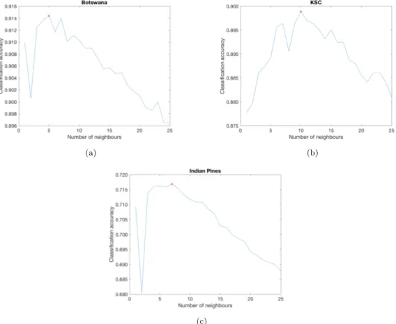
The k-nearest neighbours approach is a nonparametric classifier. It takes into con-sideration the spatial relationship amongst data points. Each new entry is classified according to its k-nearest neighbours in the feature space, being assigned the label of the majority. Different k values lead to different outcomes, so, in order to find the most suitable number of neighbours, for each k = n, with n ∈ {1, 2, ..., 25}, the KNN classification using the three images described in Section 4.1 has been performed. Each image has been analyzed separately, and the mean results are shown in Figure 4. All the spectral bands were used in order not to favor any BS method compared in this work. The best accuracy for the Botswana dataset is achieved with k = 5. For the KSC image, the best number of neighbours is k = 10. And k = 7 yields the best outcome for the Indian Pines dataset. These parameters will be kept throughout this paper. 4.2.2. CART

Classification and Regression Trees is a nonparametric classifier based on Decision Trees. Basically, it defines features thresholds in order to split the feature space into homogeneous regions. For the classification of a new entry, its features are analyzed according to the previously learned thresholds, and its label will be assigned according to the feature space region this entry falls into.

4.3. Related Works for Comparison

Results obtained by the proposed approach in this paper are compared with results from three state-of-the-art supervised band selection approaches. The framework we

(12)

(a) (b)

(c)

Figure 4.: KNN mean classification accuracies with different numbers of neighbours. In (a), the best number of neighbours (red dot) k for the Botswana image is k = 5. In (b), the best number of neighbours is k = 10. And in (c), k = 7.

(13)

propose is based on Machine Learning, so, for the sake of a more diverse comparison, we chose methods from three different branches, namely Statistical Models, Evolutionary Algorithms (EA) and Image Processing (IP).

4.3.1. Statistical Models-based Approach

In the first method (Feng et al. 2017), the authors propose a framework that uses Non-homogeneous Hidden Markov Chains (NHMC) and wavelet transform as tools for band selection. Spectral signatures are first processed by wavelet transform, which is capable of encoding compactly the locations and scales at which the signal structure is present. A zero-mean Gaussian mixture model is then used to provide discrete values for the wavelet coefficients. The more Gaussian components used, the greater the detail in the descriptors generated. However, the authors demonstrate that the accuracy obtained using just two Gaussian components is usually only 1% less than where multiple Gaussian components are used and therefore in this paper, we have limited ourselves to two in order to reduce the computational load. Since wavelet coefficient properties can be accurately modeled by a NHMC, this Hidden Markov Chain is also used. Processing yields a set of candidate bands, among which those with the highest score in terms of correlation form the final output of this framework. The authors use an SVM classifier to measure the accuracy of the resulting bands.

This is a filter-based method, because the selection of bands is done before the classification is performed by SVM. It is also a sequential search algorithm, performing a sequential forward selection.

4.3.2. EA-based Approach

The second method is based on EA (Saqui et al. 2016). More precisely, it uses a Genetic Algorithm (GA). Normally, GA methods use three operators: Selection, crossover and mutation of individuals. Each element of the population is a binary vector v ∈ N1×d0

—also called chromosome —where d0 is the number of spectral bands in the image.

Each component, or gene, vkin v indicates the presence of the kth band when vk= 1. At each generation of the algorithm, the population is evaluated by the fitness function, which is a Gaussian Maximum Likelihood Classifier. This classifier classifies the image using the bands indicated by the different vectors v , and the classification accuracy is used as the fitness of the chromosome. After each iteration, the best chromosomes are retained, following which they are subjected to crossover and mutations. The whole process is repeated until a predefined number of generations is reached. At the end, the selected fittest chromosome is the one with the selected bands.

Clearly, this is a wrapper-based method, i.e., the process of selecting features is embedded in the classifier. It also performs a random search, in virtue of the intrinsic characteristics of EA-based methods.

4.3.3. Image Processing-based Approach

The third competitor (Cao et al. 2017a) is a semi-supervised method that uses Image Processing tools in its wrapper-based band selection framework. Firstly, it trains a SVM classifier based on labeled instances, then this classifier assigns class label to un-labeled data, which end up having wrong labels —or pseudo ground-truth. After that, the resulting classification map is improved by an IP-based edge-preserving filter. At this point, there are two data sets: One with the original ground-truth information, and other with calculated pseudo ground-truth information. Then, for each combination of

(14)

Figure 5.: KNN accuracies with different percentages of Botswana training data.

candidate bands to be selected, another SVM is trained using the data with original ground-truth, and its accuracy is assessed by the data set with pseudo ground-truth. By testing several band combinations, it is possible to select the one with the highest classifier accuracy.

4.4. Results

Supervised approaches rely on labeled training data to obtain their results. As already stated, the assignment of labels to pixels is an expensive task. So, in this paper, the proposed BS framework uses only a small percentage of the available training data to get its results.

4.4.1. Percentage of the training data used

We ran the proposed band selection algorithm ten times, with different fractions of the available training data. For each percentage ps= s/100, with s ∈ {10, 20, ..., 100}, the

proposed BS method has been used to select bands, and the cardinality of its training set was |X| × ps. Thus, for each ps there is a set Ss of selected bands. Each Ss has 50

selected bands.

Using all the three images, Figure 5 shows how the KNN classifier’s mean accuracies change with different quantities of training data. In general, there is a tendency of getting higher accuracies as the amount of training data increases. With 20% of the available training data, the proposed algorithm had an accuracy similar to that of 30% and 40%. As it is desirable to work only a small fraction of the available training data, we chose to use only 20% of the data to select bands using the proposed method. 4.4.2. Methods Comparison

The bands selected by each competitor will be compared. We measure the validity of each subset of selected bands using two classifiers, namely, KNN and CART, which are largely used in classification of hyperspectral images (Wang et al. 2017a; Wang, Lin, and Yuan 2016; Zhu et al. 2017; Zhang et al. 2017).

(15)

(a) (b)

(c)

Figure 6.: (a) Mean spectral signatures for the Botswana image. (b) Mean spectral signatures for the KSC image. (c) Mean spectral signatures for the Indian Pines image.

command, from Statistics and Machine Learning toolbox. For CART, fitctree was used, also from Statistics and Machine Learning toolbox. The proposed BS framework was also implemented in Matlab, and we used the trainSoftmaxLayer command, from Neural Network Toolbox, for single-layer neural network, with 2000 training epochs—normally the training phase stopped before this, so other training epochs quantities were not tested.

First, it is important to analyze the dataset to have an idea of the complexity of the problem. Figure 6 shows the mean spectral signature of each class. In Figure 6(a), for example, it can be seen that in some regions the spectral signatures are further apart than in other regions of the electromagnetic spectrum. Since each spectral signature corresponds to a class, one might conclude intuitively that the bands where the curves are more spread out will provide a better class separability. In Figure 6(b), the spectral signatures of classes are practically juxtaposed, except in a handful of regions. This can prevent the classifier from achieving a good outcome.

The competitor described in Section 4.3.1 will be called NHMC. The method de-scribed in Section 4.3.2 will be called GA. Finally, the algorithm dede-scribed in Section 4.3.3 will be referred to as ICM.

All the classifiers results that will be exhibited in this paper are the mean values of 10 runs. Standard-deviation values are also calculated.

(16)

4.4.2.1. Botswana image. Table 1 shows the bands selected by the proposed method, SLN. In Table 2, which exhibits the KNN mean accuracies and their respective standard-deviation for Botswana image, we see that the SLN method outperformed its competitors with 20, 30, 40 and 50 bands. Figure 7 (a) gives a plot of the results of the four methods. It is then possible to see the advantage of the proposed method in almost all cases.

Table 3 shows the CART mean accuracies and standard-deviations for Botswana image. The proposed SLN method got the best results with 40 bands. Figure 7 (b) gives a visual perspective about the results.

Table 1.: Selected bands for the Botswana image. 10 bands 1 3 20 27 32 37 43 50 54 68 20 bands 1 4 7 16 20 21 24 26 31 35 37 44 47 50 57 59 62 69 93 98 30 bands 1 4 6 10 13 16 21 24 29 33 35 38 41 43 47 49 50 55 59 61 67 71 75 84 89 93 107 113 122 125 40 bands 1 4 6 10 11 13 16 21 23 24 25 27 29 32 33 35 38 40 41 43 47 49 50 52 54 55 59 61 67 71 74 75 84 89 93 106 107 112 122 125 50 bands 1 2 6 13 15 19 20 23 24 26 27 29 32 34 35 41 43 44 47 49 50 52 53 54 55 61 63 64 65 66 69 71 73 74 75 79 84 87 94 96 98 103 106 107 112 115 117 122 125 131

Table 2.: KNN results for Botswana image, in percentages. The results in bold are the highest values, and std stands for standard-deviation.

10 bands 20 bands 30 bands 40 bands 50 bands Method mean std mean std mean std mean std mean std SLN 90.86 0.58 91.19 1.13 91.09 0.91 91.16 1.10 91.22 1.15 NHMC 90.54 0.66 90.69 0.57 90.68 0.60 90.85 0.58 90.99 0.76 GA 90.95 0.72 90.89 0.69 90.75 0.53 91.00 0.76 90.89 0.67 ICM 90.52 0.71 90.54 0.71 90.26 1.14 90.32 1.02 90.51 0.88

Table 3.: CART results for Botswana image, in percentages. The highest values are emphasized in bold, and std means standard-deviation.

4.4.2.2. KSC image. In Table 4 all the bands selected by the SLN approach are displayed.

(17)

(a) (b)

Figure 7.: Botswana image accuracy results having as input bands selected by all BS methods. In (a), results achieved by the KNN classifier. In (b), results obtained by CART.

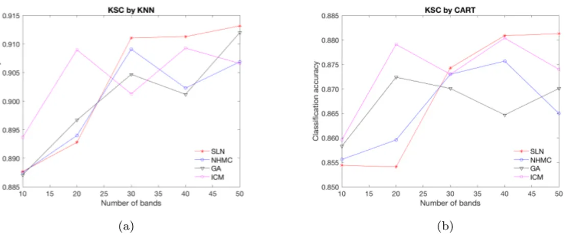
Table 5 shows the KNN mean accuracies and standard-deviation for KSC image. The proposed method SLN got the best results with 30, 40 and 50 bands. Figure 8 (a) shows the results.

In Table 6, the CART classifier results are exhibited. The same results are depicted in Figure 8 (b). The proposed method got the best results again with 30, 40 and 50 bands.

Table 4.: Selected bands for KSC image. 10 bands 1 17 34 37 48 74 98 134 161 175 20 bands 1 6 8 19 25 28 33 48 53 72 76 95 133 139 143 150 163 168 173 176 30 bands 1 2 9 15 19 28 31 34 37 41 44 47 48 72 74 75 96 97 101 110 124 133 135 139 143 147 160 163 167 175 40 bands 1 3 7 16 19 26 28 30 32 34 35 39 40 43 49 51 53 56 71 73 77 93 94 95 96 101 104 125 133 134 142 145 150 153 159 162 167 169 171 174 50 bands 1 3 7 9 18 19 26 28 33 34 37 38 39 41 42 47 48 51 53 59 68 69 70 71 72 73 78 96 97 100 101 107 110 111 120 121 125 127 131 133 135 137 140 142 143 159 162 171 173 175

4.4.2.3. Indian Pines image. The bands selected by our approach are shown in Table 7.

According to Table 8, the proposed method got the best result with 30 bands, using the KNN classifier with Indian Pines image. In Figure 9 (a), the results are displayed. In Table 9, the proposed SLN method has the best result with 30 bands. The results can be visualized in Figure 9 (b).

(18)

Table 5.: KNN results, in percentages, for KSC image. The values in bold represent the highest outcomes and std stands for standard-deviation.

Table 6.: CART results for KSC image, in percentages. The values in bold represent the highest values, and std stands for standard-deviation.

(a) (b)

Figure 8.: Classification accuracies for KSC images, having as input the bands selected by the methods under analysis. In (a), results by KNN classifier. In (b), results obtained by CART.

(19)

Table 7.: Selected bands for Indian Pines image. 10 bands 10 25 32 39 42 48 63 75 91 98 149 20 bands 5 11 18 23 25 29 36 44 52 56 60 64 75 91 94 98 106 117 132 168 30 bands 5 6 11 16 18 20 23 25 29 30 31 36 38 44 47 52 54 56 60 62 64 74 75 91 94 98 106 117 132 168 40 bands 1 8 10 12 15 19 20 23 27 30 32 36 39 41 49 51 54 56 58 60 64 66 71 74 75 80 91 94 98 101 113 117 149 156 167 170 173 178 206 218 50 bands 4 8 11 14 18 20 22 27 30 32 36 38 41 44 46 48 52 58 60 62 64 66 68 71 75 77 81 84 86 88 90 94 95 98 100 109 117 124 137 140 149 153 156 167 170 172 174 178 202 216

Table 8.: KNN results, in percentages, for Indian Pines image. The highest values are in bold, and std means standard-deviation.

Table 9.: CART results for Indian Pines image, in percentages. The highest values are in bold, and std stands for standard-deviation.

(20)

(a) (b)

Figure 9.: Indian Pines image classification results by KNN classifier. In (a), KNN results. In (b), results achieved by CART.

4.4.3. Linear separation in a one-vs-all scheme

As we use a linear classifier in the proposed framework, all the results and their subsequent analyses are only valid if the classification problem to be solved is also linear.

In a one-vs-all scheme, in many cases the two groups are linearly separable. There are other situations in which a hyperplane cannot separate the two classes, however it may still provide a reasonable separation. To illustrate this, in Figure 10, all the 14 classes present in the Botswana image data set are displayed in a one-vs-all fashion. We reduced the data dimensionality by using the first two principal components from the Principal Components Analysis. The data samples in green color represent the class j under analysis, for j = 1, ..., 14, and the blue points stand for a balanced composition of the remaining classes. Thus, for each frame in Figure 10, the number of green and blue points is practically the same. The red line segment in each frame represents the separating boundary provided by a single-layer neural network.

4.5. Remarks about the results 4.5.1. KNN versus CART

Both classifiers used in this paper are nonparametric, that is, they do not assume any hypothesis about data distribution nor about its parameters. Yet, they share more dissimilarities than characteristics in common. To illustrate this, one can notice the differences between the overall accuracies of the two classifiers, taking into account all the methods compared in this paper using the three hyperspectral images: For KNN, the mean accuracies of all results are 84.03%, whereas CART has 81.18% of mean accuracy. One possible explanation may be related to the highly nonlinearity of the classes boundaries. For example, let hl be a homogeneous region of the feature space

defined by CART, whose a new entry xi will be classified as cl, even if it belongs

to class cj. This, obviously, is a classification error. KNN classifier, in this situation,

would inquire the k nearest neighbours of xi, and eventually assign the cj label to it.

The overall results for each number of selected bands can be seen in Figure 11. For the CART classifier, the classification accuracy increased as the number of bands increased. For the KNN classifier, there was an opposite effect. This indicates that

(21)

Figure 10.: One-vs-all illustration for each class of the Botswana image. In each frame, the horizontal and vertical axis are, respectively, the first (PC1) and the second (PC2) principal components. The green dots represent the class under scrutiny, whereas the blue ones stand for data samples of the remaining classes. The red line segment is given by a single-layer neural network.

(22)

Figure 11.: Overall results considering all methods compared in this paper, using all the three images.

CART is not susceptible to the curse of dimensionality, at least in the dimensions and with the analyzed images. In general, one can see that there is not a general improvement in results as the number bands increases from 10 to 50, as shown in Figure 13.

4.5.2. Filter versus Wrapper-based Approaches

It is frequently stated in the literature that wrapper-based methods are superior in performance to filter approaches (Cao et al. 2017a; Theodoridis and Koutroumbas 2008; Shahana and Preeja 2016; Molina, Belanche, and Nebot 2002; Cao, Xiong, and Jiao 2016; Ma et al. 2017). Concerning the methods compared in this paper, SLN and NHMC are filter-based approaches; and GA and ICM are wrapper frameworks, using, respectively, Gaussian Maximum Likelihood and SVM classifiers in their frameworks. In Figure 12, the mean results of all methods are displayed. It uses all the three images with both classifiers. We analyze all the three hyperspectral datasets together just to have an idea of the general behavior each BS method, thus, it is possible to predict the methods’ performances with other HSIs. In sum, Figure 12 shows the mean values of the Tables 2, 3, 5, 6, 8 and 9. It is evident that the wrapper methods are not necessarily better than filter approaches. More precisely, the wrapper methods yield better results in only two situations—with 10 and 20 bands—, and in the remaining cases filter methods have a superior performance.

It is worth noting that a wrapper-based method proceeds to the band selection by using a certain classifier, and this classifier is supposed to be used during the subsequent classification process. It was not the case here. That is, the two wrapper competitors were trained with one classifier and used in this paper with another one, and this fact may explain why those two methods could not outperform the filter-based frameworks. On the other hand, filter methods perform the BS task without any relation with the classifier, what makes them more versatile compared to wrapper approaches.

(23)

Figure 12.: Mean results of each method, using all images and both classifiers.

4.5.3. Methods comparison

In general, as we can see in Figures 7, 8 and 9, all the four methods have their best and worst results in different situations. Thus, pointing out the best framework would not be an easy task.

In Figure 12, we can see the mean results of the four methods. The proposed method, SLN, has the best mean results using 30 and 40 spectral bands. If we take the mean value of all results—using the three images, both classifiers and also all bands—, the results are thus:

NHMC: 83.21%; ICM: 82.96%; SLN: 82.81%; and GA: 81.45%.

Basically, NHMC framework has the best overall result because it gets very high accuracies with more spectral bands. However, it does not achieve good results with less bands. Thus, NHMC has a instable behavior as the number of bands changes.

For the sake of a fair comparison, we will count how many times each method yields the best results—values in bold in Tables 2, 3, 5, 6, 8 and 9. In this case, we have the following outcome:

SLN: 13; ICM: 10; GA: 5; and NHMC: 2.

Consequently, one can infer that our proposed method has a stable outcome, achiev-ing the best results in 43.33% of the tests.

It is worth-mentioning that, in most cases, the BS methods have very similar results that can be considered equal, in terms of statistical significance. However, in this section we insist on ranking the band selection frameworks just to have a way to compared them.

4.5.4. Discussions on the proposed method

As shown in Figure 12, the proposed method has a tendency of achieving better results as the number of selected bands increases from 10 until 30. It is important to notice that each time the single-layer neural network is used to select bands, its training phase starts with random values for weights and bias. Thus, two distinct runs are not likely to have the same outcome. One possible explanation for this decrease from the 30thband

(24)

Figure 13.: Mean accuracies of all results by both classifiers in relation to the number of selected bands. All the three images are used.

may be related to the random initialization of our framework. Furthermore, due to the peaking phenomenon—or curse of dimensionality—(Theodoridis and Koutroumbas 2008), the classification accuracy increases as more spectral bands are used until a critical point, after which the probability of error increases. This explains the fact that the accuracy of the SLN method decreases for 40 and 50 bands.

In order to see that, refer to Figure 13, which shows the overall results of all methods together, using the three images and both classifiers. In general, the accuracies increase until a certain point, after which they start decreasing. The peak in the 20 bands region is due to the high scores achieved by the ICM method, as already shown in Figure 12. As already said in Section 3.2.4, there is not a minimum limit of bands to be selected by SLN. However, Figure 12 shows that SLN achieves below-average results with 10 and 20 bands. When it comes to the 10-bands case, we may conclude that its poor results—compared to its competitors—may be due to the fact that SLN does not inquiry all the classes of band selection when σ < q.

Using 30 bands, the proposed method gets above-average results, as shown in Figure 12. In this case, all the classes were inquired during the BS process. Consequently, better results were achieved.

Finally, we should bear in mind that all the proposed method’s results were attained by using only 20% of the available training data. Besides, the simplicity of the proposed method, in terms of implementation, makes it a good choice in the feature selection area.

5. Conclusion

Hyperspectral images provide rich spectral information about the scene under analysis as a result of their both numerous and contiguous bands. Since different materials have distinct spectral signatures, objects with similar characteristics in terms of colors and shape may still be distinguished in the spectral domain.

One issue to be taken into account is the high correlation between neighbouring bands, which causes data redundancy. The ratio amongst training patterns and free classifier parameters is meaningful for classifiers, and so decreasing the dimensionality

(25)

of data can avoid overfitting.

One way of handling this dimensionality reduction is band selection. One positive aspect of BS is that it retains the original information, which can be very useful in some cases.

In this context, the present paper proposed a supervised filter-based band selec-tion framework based on single-layer neural networks using only 20% of the available training data. For each class in the data set a binary classification into class and non-class was performed, and the bands corresponding to the largest and smallest weights were selected. During this iterative process, the bands most correlated with the bands selected are automatically discarded, according to a procedure also proposed in this letter. In general, the proposed method may be seen as a class-oriented band selection approach, allowing a BS criterion that meets the needs of each class.

A number of other filter-based BS algorithms perform their choice of bands based, for instance, on statistical properties of the data set. A positive aspect of the filter-based method proposed in this paper is that it is filter-based on classification, that is, uses a linear classifier to rank and select the bands. The proposed method outperformed its competitors in 43.33% of the cases analyzed in this paper.

As a secondary conclusion, we showed that wrapper-based approaches are not neces-sarily better than their filter counterparts, when using different classifiers for the band selection process and for the classification. More research on this subject is necessary. A next step is to devise a methodology in order to find the optimum number of bands to be selected for a given application and image.

References

Bai, J., S. Xiang, L. Shi, and C. Pan. 2015. “Semisupervised Pair-Wise Band Selection for Hyperspectral Images.” IEEE Journal of Selected Topics in Applied Earth Observations and Remote Sensing 8 (6): 2798–2813.

Bai, X., Z. Guo, Y. Wang, Z. Zhang, and J. Zhou. n.d. IEEE Journal of Selected Topics in Applied Earth Observations and Remote Sensing (6): 2774–2783.

Bishop, Christopher M. 2006. Pattern Recognition and Machine Learning. Springer. http://research.microsoft.com/en-us/um/people/cmbishop/prml/.

Bris, A. Le, N. Chehata, X. Briottet, and N. Paparoditis. 2014. “Use intermediate results of wrapper band selection methods: A first step toward the optimization of spectral config-uration for land cover classifications.” In 2014 6th Workshop on Hyperspectral Image and Signal Processing: Evolution in Remote Sensing (WHISPERS), June, 1–4.

Camps-Valls, G., J. Mooij, and B. Scholkopf. 2010. “Remote Sensing Feature Selection by Kernel Dependence Measures.” IEEE Geoscience and Remote Sensing Letters 7 (3): 587– 591.

Cao, X., C. Wei, J. Han, and L. Jiao. 2017a. “Hyperspectral Band Selection Using Improved Classification Map.” IEEE Geoscience and Remote Sensing Letters PP (99): 1–5.

Cao, X., T. Xiong, and L. Jiao. 2016. “Supervised Band Selection Using Local Spatial In-formation for Hyperspectral Image.” IEEE Geoscience and Remote Sensing Letters 13 (3): 329–333.

Cao, Xianghai, Jungong Han, Shuyuan Yang, Dacheng Tao, and Licheng Jiao. 2016. “Band selection and evaluation with spatial information.” International Journal of Remote Sensing 37 (19): 4501–4520. https://doi.org/10.1080/01431161.2016.1214301.

Cao, Xianghai, Xinghua Li, Zehan Li, and Licheng Jiao. 2017b. “Hyperspectral band selection with objective image quality assessment.” International Journal of Remote Sensing 38 (12): 3656–3668. https://doi.org/10.1080/01431161.2017.1302110.

(26)

selection.” In 2015 International Joint Conference on Neural Networks (IJCNN), July, 1–6. Cover, T. M. 1965. “Geometrical and Statistical Properties of Systems of Linear Inequalities with Applications in Pattern Recognition.” IEEE Transactions on Electronic Computers EC-14 (3): 326–334.

Cui, M., S. Prasad, M. Mahrooghy, L. M. Bruce, and J. Aanstoos. 2011. “Genetic algorithms and Linear Discriminant Analysis based dimensionality reduction for remotely sensed image analysis.” In 2011 IEEE International Geoscience and Remote Sensing Symposium, July, 2373–2376.

Damodaran, B. B., N. Courty, and S. Lefevre. 2017. “Sparse Hilbert Schmidt Independence Criterion and Surrogate-Kernel-Based Feature Selection for Hyperspectral Image Classifi-cation.” IEEE Transactions on Geoscience and Remote Sensing 55 (4): 2385–2398.

Das, Sanmay. 2001. “Filters, Wrappers and a Boosting-Based Hybrid for Feature Selec-tion.” In Proceedings of the Eighteenth International Conference on Machine Learn-ing, ICML ’01, San Francisco, CA, USA, 74–81. Morgan Kaufmann Publishers Inc. http://dl.acm.org/citation.cfm?id=645530.658297.

Dong, Y., B. Du, L. Zhang, and L. Zhang. 2017. “Dimensionality Reduction and Classification of Hyperspectral Images Using Ensemble Discriminative Local Metric Learning.” IEEE Transactions on Geoscience and Remote Sensing 55 (5): 2509–2524.

Du, Q., and H. Yang. 2008. “Similarity-Based Unsupervised Band Selection for Hyperspectral Image Analysis.” IEEE Geoscience and Remote Sensing Letters 5 (4): 564–568.

Duda, Richard O., Peter E. Hart, and David G. Stork. 2001. Pattern Classification (2nd Ed). Wiley.

ElMasry, Gamal, and Da-Wen Sun. 2010. “Chapter 1 - Principles of Hyper-spectral Imaging Technology.” In HyperHyper-spectral Imaging for Food Quality Analy-sis and Control, edited by Da-Wen Sun, 3 – 43. San Diego: Academic Press. http://www.sciencedirect.com/science/article/pii/B9780123747532100012.

Fauvel, M., C. Dechesne, A. Zullo, and F. Ferraty. 2015. “Fast Forward Feature Selection of Hyperspectral Images for Classification With Gaussian Mixture Models.” IEEE Journal of Selected Topics in Applied Earth Observations and Remote Sensing 8 (6): 2824–2831. Feng, S., Y. Itoh, M. Parente, and M. F. Duarte. 2017. “Hyperspectral Band Selection From

Statistical Wavelet Models.” IEEE Transactions on Geoscience and Remote Sensing 55 (4): 2111–2123.

Habermann, M., V. Fremont, and E. H. Shiguemori. 2017. “Problem-based band selection for hyperspectral images.” In 2017 IEEE International Geoscience and Remote Sensing Symposium (IGARSS), July, 1800–1803.

Hastie, Trevor, Robert Tibshirani, and Martin Wainwright. 2015. Statistical Learning with Sparsity: The Lasso and Generalizations. Chapman & Hall/CRC.

Jahanshahi, S. 2016. “Maximum relevance and class separability for hyperspectral feature selection and classification.” In 2016 IEEE 10th International Conference on Application of Information and Communication Technologies (AICT), Oct, 1–4.

Jiang, J., L. Huang, H. Li, and L. Xiao. 2016. “Hyperspectral image supervised classification via multi-view nuclear norm based 2D PCA feature extraction and kernel ELM.” In 2016 IEEE International Geoscience and Remote Sensing Symposium (IGARSS), July, 1496–1499. Jiao, L., J. Feng, F. Liu, T. Sun, and X. Zhang. 2015. “Semisupervised Affinity Propagation

Based on Normalized Trivariable Mutual Information for Hyperspectral Band Selection.” IEEE Journal of Selected Topics in Applied Earth Observations and Remote Sensing 8 (6): 2760–2773.

Keshava, N. 2004. “Distance metrics and band selection in hyperspectral processing with appli-cations to material identification and spectral libraries.” IEEE Transactions on Geoscience and Remote Sensing 42 (7): 1552–1565.

Khalid, S., T. Khalil, and S. Nasreen. 2014. “A survey of feature selection and feature extraction techniques in machine learning.” In 2014 Science and Information Conference, Aug, 372– 378.

(27)

Intelligent Systems 32 (2): 9–15.

Liu, Z., B. Tang, X. He, Q. Qiu, and H. Wang. 2017. “Sparse Tensor-Based Dimensional-ity Reduction for Hyperspectral Spectral-Spatial Discriminant Feature Extraction.” IEEE Geoscience and Remote Sensing Letters 14 (10): 1775–1779.

Luo, F., H. Huang, Y. Yang, and Z. Lv. 2016. “Dimensionality reduction of hyperspectral im-ages with local geometric structure Fisher analysis.” In 2016 IEEE International Geoscience and Remote Sensing Symposium (IGARSS), July, 52–55.

Ma, L., M. Li, Y. Gao, T. Chen, X. Ma, and L. Qu. 2017. “A Novel Wrapper Approach for Feature Selection in Object-Based Image Classification Using Polygon-Based Cross-Validation.” IEEE Geoscience and Remote Sensing Letters 14 (3): 409–413.

Marino, G., D. Tarchi, V. Kyovtorov, J. Figueiredo-Morgado, and P. F. Sammartino. 2015. “Class separability and features selection: GB-MIMO SAR MELISSA case of study.” In 2015 IEEE International Geoscience and Remote Sensing Symposium (IGARSS), July, 377–380. Martnez-UsMartinez-Uso, A., F. Pla, J. M. Sotoca, and P. Garca-Sevilla. 2007. “Clustering-Based Hyperspectral Band Selection Using Information Measures.” IEEE Transactions on Geoscience and Remote Sensing 45 (12): 4158–4171.

Molina, L. C., L. Belanche, and A. Nebot. 2002. “Feature selection algorithms: a survey and experimental evaluation.” In 2002 IEEE International Conference on Data Mining, 2002. Proceedings., 306–313.

Monteiro, S. T., and R. J. Murphy. 2011. “Embedded feature selection of hyperspectral bands with boosted decision trees.” In 2011 IEEE International Geoscience and Remote Sensing Symposium, July, 2361–2364.

Patra, S., P. Modi, and L. Bruzzone. 2015. “Hyperspectral Band Selection Based on Rough Set.” IEEE Transactions on Geoscience and Remote Sensing 53 (10): 5495–5503.

Pawlak, Zdzislaw. 1992. Rough Sets: Theoretical Aspects of Reasoning About Data. Norwell, MA, USA: Kluwer Academic Publishers.

Pessoa, A. S. Aguiar, S. Stephany, and L. M. Garcia Fonseca. 2011. “Feature selection and image classification using rough sets theory.” In 2011 IEEE International Geoscience and Remote Sensing Symposium, July, 2904–2907.

Ren, Y., L. Liao, S. J. Maybank, Y. Zhang, and X. Liu. 2017. “Hyperspectral Image Spectral-Spatial Feature Extraction via Tensor Principal Component Analysis.” IEEE Geoscience and Remote Sensing Letters 14 (9): 1431–1435.

Saqui, D., J. H. Saito, L. A. D. C. Jorge, E. J. Ferreira, D. C. Lima, and J. P. Herrera. 2016. “Methodology for Band Selection of Hyperspectral Images Using Genetic Algorithms and Gaussian Maximum Likelihood Classifier.” In 2016 International Conference on Computa-tional Science and ComputaComputa-tional Intelligence (CSCI), Dec, 733–738.

Schmidhuber, Jrgen. 2015. “Deep learning in neural networks: An overview.” Neural Networks 61: 85 – 117. http://www.sciencedirect.com/science/article/pii/S0893608014002135. Schowengerdt, Robert A. 2006. Remote Sensing, Third Edition: Models and Methods for Image

Processing. Orlando, FL, USA: Academic Press, Inc.

Serpico, S. B., and L. Bruzzone. 2001. “A new search algorithm for feature selection in hyper-spectral remote sensing images.” IEEE Transactions on Geoscience and Remote Sensing 39 (7): 1360–1367.

Shahana, A. H., and V. Preeja. 2016. “Survey on feature subset selection for high dimensional data.” In 2016 International Conference on Circuit, Power and Computing Technologies (ICCPCT), March, 1–4.

Su, H., Y. Cai, and Q. Du. 2017. “Firefly-Algorithm-Inspired Framework With Band Selection and Extreme Learning Machine for Hyperspectral Image Classification.” IEEE Journal of Selected Topics in Applied Earth Observations and Remote Sensing 10 (1): 309–320. Su, H., Q. Du, G. Chen, and P. Du. 2014. “Optimized Hyperspectral Band Selection Using

Par-ticle Swarm Optimization.” IEEE Journal of Selected Topics in Applied Earth Observations and Remote Sensing 7 (6): 2659–2670.

Su, H., H. Yang, Q. Du, and Y. Sheng. 2011. “Semisupervised Band Clustering for Dimension-ality Reduction of Hyperspectral Imagery.” IEEE Geoscience and Remote Sensing Letters

(28)

8 (6): 1135–1139.

Su, H., B. Yong, and Q. Du. 2016. “Hyperspectral Band Selection Using Improved Firefly Algorithm.” IEEE Geoscience and Remote Sensing Letters 13 (1): 68–72.

Su, Hongjun, and Qian Du. 2012. “Hyperspectral band clustering and band selec-tion for urban land cover classificaselec-tion.” Geocarto Internaselec-tional 27 (5): 395–411. https://doi.org/10.1080/10106049.2011.643322.

Sui, C., Y. Tian, Y. Xu, and Y. Xie. 2015. “Unsupervised Band Selection by Integrating the Overall Accuracy and Redundancy.” IEEE Geoscience and Remote Sensing Letters 12 (1): 185–189.

Sun, W., L. Tian, Y. Xu, D. Zhang, and Q. Du. 2017. “Fast and Robust Self-Representation Method for Hyperspectral Band Selection.” IEEE Journal of Selected Topics in Applied Earth Observations and Remote Sensing 10 (11): 5087–5098.

Sun, W., L. Zhang, L. Zhang, and Y. M. Lai. 2016. “A Dissimilarity-Weighted Sparse Self-Representation Method for Band Selection in Hyperspectral Imagery Classification.” IEEE Journal of Selected Topics in Applied Earth Observations and Remote Sensing 9 (9): 4374– 4388.

Theodoridis, Sergios, and Konstantinos Koutroumbas. 2008. Pattern Recognition, Fourth Edi-tion. 4th ed. Academic Press.

Wang, J., K. Zhang, P. Wang, K. Madani, and C. Sabourin. 2017a. “Unsupervised Band Se-lection Using Block-Diagonal Sparsity for Hyperspectral Image Classification.” IEEE Geo-science and Remote Sensing Letters PP (99): 1–5.

Wang, L., C. I. Chang, L. C. Lee, Y. Wang, B. Xue, M. Song, C. Yu, and S. Li. 2017b. “Band Subset Selection for Anomaly Detection in Hyperspectral Imagery.” IEEE Transactions on Geoscience and Remote Sensing 55 (9): 4887–4898.

Wang, Q., J. Lin, and Y. Yuan. 2016. “Salient Band Selection for Hyperspectral Image Clas-sification via Manifold Ranking.” IEEE Transactions on Neural Networks and Learning Systems 27 (6): 1279–1289.

Xia, J., L. Bombrun, Y. Berthoumieu, C. Germain, and P. Du. 2017. “Spatial Rotation Forest for Hyperspectral Image Classification.” IEEE Journal of Selected Topics in Applied Earth Observations and Remote Sensing 10 (10): 4605–4613.

Xu, X., J. Li, and S. Li. 2017. “Multiview Intensity-Based Active Learning for Hyperspectral Image Classification.” IEEE Transactions on Geoscience and Remote Sensing PP (99): 1– 12.

Xu, X., Z. Shi, and B. Pan. 2017. “A New Unsupervised Hyperspectral Band Selection Method Based on Multiobjective Optimization.” IEEE Geoscience and Remote Sensing Letters PP (99): 1–5.

Yuan, Y., G. Zhu, and Q. Wang. 2015. “Hyperspectral Band Selection by Multitask Sparsity Pursuit.” IEEE Transactions on Geoscience and Remote Sensing 53 (2): 631–644.

Zhan, Y., D. Hu, H. Xing, and X. Yu. 2017. “Hyperspectral Band Selection Based on Deep Convolutional Neural Network and Distance Density.” IEEE Geoscience and Remote Sens-ing Letters 14 (12): 2365–2369.

Zhang, M., Jingjing Ma, M. Gong, Hao Li, and Jia Liu. 2017. “Memetic algorithm based feature selection for hyperspectral images classification.” In 2017 IEEE Congress on Evolutionary Computation (CEC), June, 495–502.

Zhu, G., Y. Huang, S. Li, J. Tang, and D. Liang. 2017. “Hyperspectral Band Selection via Rank Minimization.” IEEE Geoscience and Remote Sensing Letters 14 (12): 2320–2324. cal, M., K. Ergn, and G. B. Akar. 2017. “Comparative analysis of hyperspectral feature

ex-traction methods in vegetation classification.” In 2017 25th Signal Processing and Commu-nications Applications Conference (SIU), May, 1–4.