Science Arts & Métiers (SAM)
is an open access repository that collects the work of Arts et Métiers Institute of Technology researchers and makes it freely available over the web where possible.
This is an author-deposited version published in: https://sam.ensam.eu Handle ID: .http://hdl.handle.net/10985/8737
To cite this version :
Mathieu HOBON, Nafissa LAKBAKBI EL YAAQOUBI, Gabriel ABBA - Quasi optimal sagittal gait of a biped robot with a new structure of knee joint - Robotics and Autonomous Systems - Vol. 62, n°4, p.436-445 - 2013
Quasi optimal sagittal gait of a biped robot with a new
structure of knee joint
M. Hobona,∗, N. Lakbakbi Elyaaqoubia,b, G. Abbaa,b
adesign Manufacturing and Control Laboratory, EA 4495, ENSAM CER Metz, 4 rue
Augustin Fresnel, 57078 Metz Cedex 3, France
bNational Engineering School of Metz, 1 route d’Ars Laquenexy, 57078 Metz Cedex 3,
France
Abstract
The design of humanoid robots has been a tricky challenge for several years. Due to the kinematic complexity of human joints, their movements are noto-riously difficult to be reproduced by a mechanism. The human knees allow movements including rolling and sliding, and therefore the design of new bio-inspired knees is of utmost importance for the reproduction of anthro-pomorphic walking in the sagittal plane. In this article, the kinematic char-acteristics of knees were analyzed and a mechanical solution for reproducing them is proposed. The geometrical, kinematic and dynamic models are built together with an impact model for a biped robot with the new knee kine-matic. The walking gait is studied as a problem of parametric optimization under constraints. The trajectories of walking are approximated by mathe-matical functions for a gait composed of single support phases with impacts. Energy criteria allow comparing the robot provided with the new rolling knee mechanism and a robot equipped with revolute knee joints. The results of the optimizations show that the rolling knee brings a decrease of the sthenic criterion. The comparisons of torques are also observed to show the difference of energy distribution between the actuators. For the same actuator selec-tion, these results prove that the robot with rolling knees can walk longer than the robot with revolute joint knees.
Keywords: biped robot, optimal gait, dynamic model, humanoid design, ∗Principal corresponding author
Email addresses: mathieu.hobon@ensam.eu (M. Hobon), lakbakbi@enim.fr
rolling contact knees
1. Introduction
Over the last several years, the design and the control of biped and hu-manoid robots has been a research track attracting many researchers. A humanoid robot is an autonomous mobile system that needs to be capable of transporting energy and of course its structure and actuators. Walking is a principle of displacement in itself. From the beginning the design must therefore integrate that during the walking the robot must be capable of supporting the weight of the structure and actuators as well as the source of energy. The primary objective of this paper is to verify that the actuators required to perform different walking gaits have a lower mass than expected in the initial design. In addition, this study provides reference trajectories for the control and data on the robot walking. The second objective of this work is to study the kinematics of the knee and its influence on the performance of the robot.
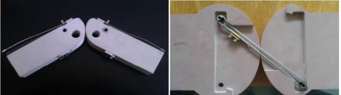
Generally, the knee joints of numerous humanoids robots are simple revo-lute joints. The corresponding configuration is denoted CK robot hereinafter. The methods improving these joints have been investigated by researchers in [1] [2] and [3]. Van Oort et al. [1] introduced a device with 4-bar knees ca-pable of minimizing the energy consumption of the knee’s actuators through locking the knee when the support leg is stretched. Hamon and Aoustin [2] studied a cross four-bar mechanical linkage. They focused on the comparison using the same criteria between two kinematic structures of walking robots: one with classic revolute joint and the other with cross four-bar joint at the knees. The results indicated that the four-bar structure can reduce energy consumption and the forces due to the foot impact on the ground decrease. Finally in the project LARP, Gini et al. [3] designed a pin joint with a mov-ing center of rotation along two cylindrical surfaces. However, the detailed reduction in energy consumption using the pin joint was not stated in their published work [3]. The joint consisting of two cylindrical surfaces rolling one on the other is called thereafter rolling knee and denoted RK. In [4], the authors suggest several solutions to design a rolling knee. A solution including tendons is indicated, as well as different motorization options. As example of possible realization of the joint with tendon, two pictures of the prototype realized in the laboratory are given in Fig. 1
Figure 1: Picture of the prototypes
In general, a walking gait consists of various phases of support (single and double supports) and impact phases. Thus, the robot dynamics is described by a set of hybrid non-linear equations. The selections of a robot’s kinematic structure, its dimensions, its actuators and its control laws are determined by the optimization methodology. It is really important to find an effective optimization criterion. At present, there are several published criteria avail-able [2] [5] [6] and [7]. The criterion most frequently adopted is a quadratic criterion derived from the optimal control techniques. The criterion, named sthenic criterion, is based on the sum of the squares of the actuator torques [5] [8]. Because Joule losses are directly related to the square of the couples, the overall performance can be obtained simply by weighting the previous criterion. Srinivasan [6] proposed, as criteria, the cost indicated by the mean square of muscles forces, relating to the sthenic criterion, or the metabolic cost of muscle contraction power, relating to an energy criterion. The tra-jectory can also be defined by the displacement of the robot’s center of mass using walking patterns [6] or based on the stable gait primitive [9].
The optimization of the dynamics of a non-linear hybrid system is quite complicated. To solve the problem, one can use the approach with direct methods that consist in solving the discretized problem by using paramet-ric optimization techniques. Direct methods can be classified in three ap-proaches: (i) Collocation methods, (ii) Multiple-shooting methods, and (iii) Methods based on parametrization of the state variables by using functions like B-spline or cubic spline functions [10] [11]. A parametrization method was used by [12], [13], [8] who have attained good results.
We chose the third method, the parametrization of the state vector. The problem consequentially becomes a parameter optimization satisfying the non-linear hybrid dynamic equations and the walking constraints of the robot
[14]. These constraints, which must be satisfied, encompass a non-contact requirement for the mobile foot above the ground, the unilateral contact of the fixed foot, the hypothesis in accordance with the impact of mobile foot and the stability of the robot defined by the ZMP position.
The minimization problem can be resolved in many ways. If we provide explicit expressions of the gradient and the Hessian of the criterion, we can use a very simple algorithm such as the gradient method or Newton method [8] [15] [10]. Constraints are nonlinear in the parameters and the impact equation leads to a reduced area of solutions. Moreover, to obtain low com-putation time, these methods often require the explicit calculation of the gradient of the cost function [15]. Genetic algorithms [16] or evolutionary al-gorithms will be more effective but their convergence time is long. Moreover, we do not have here a large number of parameters.
The Nelder-Mead simplex algorithm is another direct search method. [17] has proved the convergence properties in low dimensions. [18] has given a counterexample for a very particular function. We do not have this prob-lem in our case. On the other hand, the simplex algorithm requires adding constraints in criterion with Lagrange multipliers.
In this paper, we intend to study the advantages of an anthropomorphic knee kinematic structure by searching for the inner correlation between dif-ferent gaits and the energy they consume. Optimization methodologies based on the model of inverse pendulum and rigid knees proposed by Srinvasan [6] and Park et al [19] are no longer supported by our model. We confine our robots to a configuration of 7 links, namely, a trunk, two thighs, two shins and two feet. In order to highlight the effectiveness of the new kinematic structure brought by our knees, we do not consider the utilization of springs and compliant devices on robot joints.
In this paper, we compare the evolution of the energy criteria of two kine-matic structures of knees on a robot using different trajectories. The first structure uses classic revolute knees and the second one uses knees with cylin-drical rolling contact. The corresponding geometric, kinematic and dynamic models have been developed for these two structures in Section 2. The opti-mization problem is discussed in Section 3 and two types of trajectories for the gait have been developed in Section 4. According to the results generated in Section 5, we can decide if our new kinematic solution for the knees truly consumes less energy during the cyclic walking. The optimized trajectories with less energy consumption will be used to improve the control strategies of the walking robots. The selection of the criterion is given by the sthenic
function since it is better adapted for the future of the project and for the stabilizing control.
2. The biped modelling
q3 Cg2 q2 q6 Cg6 H Cg3 K2 N O0 Cg1 q1 T1 H1 x0 z0 y0 K1 A1 G 1 G2 G3 G4 G5 T2 Cg4 q4 H2 A2 z5 x5 q5 G6
Figure 2: Biped robot with rolling joint knees
2.1. The Biped and the new knee kinematic
The studied robot consists of seven bodies, namely two feet, two shins, two thighs and a trunk. We consider hereafter two configurations that differ at the knee kinematics. The first configuration possesses a revolute joint on the knee as most of the biped robots and humanoids realized until now [20]. The second configuration possesses a knee with a rolling contact as repre-sented on Fig. 2. We suppose hereafter that the contact of the link between the shin and the thigh is made without sliding. The robot is supplied with six actuators placed at the rotation axis of every joint. We define the inertial ref-erence frame R0 = (O0, ⃗x0, ⃗y0, ⃗z0) related to the foot 1 with the origin O0 the projection of the point A1 on the ground, supposed horizontal, ⃗x0 is the unit vector in the gait direction and ⃗z0the unit vector perpendicular to the ground
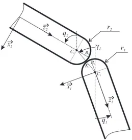
g1 q1 q2 C2 z2 x1 z1 r2 C1 r1 B2 B1 K1 x2
Figure 3: Rolling knee of the support leg
plane. The two configurations are defined in the sagittal plane by the absolute angular coordinates named Xe = [q⊤ xH zH]⊤ with (xH, zH) the hip
Carte-sian coordinates in R0 and q⊤ = [q0, q1, q2, q3, q4, q5, q6] the vector of absolute joint angles. The joint torque vector is defined by Γ = [Γ1, Γ2, Γ3, Γ4, Γ5, Γ6]⊤ as represented on Fig. 2. The joint torques are applied around the axis ⃗y.
Defining θ = [q1−q0, q2−q1, q6−q2, q6−q3, q3−q4, q4−q5]⊤ the joint angular position vector.
For the robot structure with revolute joints, the coordinates of the hip are given by the equations:
xH = −l2sin q2 − l1sin q1 (1)
zH = l2cos q2 + l1cos q1 + hp (2)
with dist(A1, K1) = dist(A2, K2) = l1 the length of the shins, dist(K1, H) = dist(K2, H) = l2 the length of the thigh and dist(O0, A1) = hp the height of
the ankle axis.
However, in the second configuration, in addition to the revolute joints on hips and ankles, the knees contain a rolling contact cylinder on cylinder without sliding between the thigh and the shin. This new structure brings a coupling between the angles of the thigh q2 and of the shin q1. Fig. 3 shows the knee of leg 1. It is assumed that the knee is in contact, connected by a bar with revolute joints on the points C1 and C2. The rotation without
sliding of the shin on the thigh also leads to the rotation of the bar of an angle γ1 with reference to the vertical and given by (3). Also, the equation (4) gives the corresponding angle γ2 for the mobile leg.
γ1 = r1q1+ r2q2 r1+ r2 (3) γ2 = r1q4+ r2q3 r1+ r2 (4) From the kinematic relations and coordinates noted on figures, we can establish the direct and inverse geometric models of both robots. The coor-dinates of the hip of the structure in Fig. 2 are given by the equations:
x′H = −l2′ sin q2 − l sin γ1− l1′ sin q1 (5)
zH′ = l2′ cos q2 + l cos γ1+ l′1cos q1 + hp (6)
with l = r1+ r2. The length l′2 = l2− r2 and l′1 = l1− r1 are chosen so as to have robots of the same height for the two configurations. For the dynamic model, we assume that the centers of mass of the bodies are situated on the same position in vertical stance for both robots.
2.2. The dynamic model
The dynamic model of the robot establishes the relation between the positions, speeds and accelerations of the bodies of the robot, the torques supplied by actuators and interaction forces with its environment. The dy-namic model is usually used for the synthesis of the control laws and the stabilization of the robot, but also to determine the energy consumption of actuators, the mechanical constraints at the joints and actuators, the maxi-mal stresses to which the bodies are subjected. For each gait mode (walking, running, jump, etc.), the dynamic model allows to determine the operating point of actuators and deduce therefore their thermal stresses, the energy losses and the variation of the energy level in the batteries.
When considering only the relations between the dynamics of the bodies, the actuator torques and the external forces, the model is determined by the application of Newton’s second law. A direct explicit relation is obtained by the Euler-Lagrange equations. The rigid bodies of the robot are usually represented by their mass, the position of their center of mass and their inertia matrix. The robot studied here is a planar biped. Furthermore,
we assume that its interaction with the environment is limited to contact between the ground and the foot soles.
For the sake of simplicity, we consider a simple point-mass model for all the bodies. This hypothesis reduces the parameters defining the model for each body which are thus the mass mi and the positions si = dist(OiCgi) of
center of mass Cgi (see Fig. 2).
Finally, the application of the Euler-Lagrange equations gives the well-known differential equation of behavior of the robot ([21] and [22]) which can be expressed as:
D(Xe) ¨Xe+ H( ˙Xe, Xe) + Q(Xe) = BΓ + AcL(Xe)⊤FL+ AcR(Xe)⊤FR (7)
with D(Xe) the 9×9 inertia matrix, H( ˙Xe, Xe) the 9×1 vector of centrifugal
and Coriolis forces, Q(Xe) the 9× 1 vector due to the gravity, B the 9 × 6
control matrix, Γ the 6× 1 vector of torques, AcL and AcR the 3× 9 Jacobian
matrix of external forces and FL and FR the vectors of external wrench
respectively on the left and right feet.
Now, we analyze only the robot behavior during trajectories composed by a succession of simple support phase (SSP) followed by an impact of one foot on the ground. Assuming the left foot is on support on the ground during the SSP. The force on the right foot is zero, so FR = 0. The unknowns of
equation (7) are the coordinates of vector Xe and the vector of the external
forces FL, so we have 12 unknowns. The contact of the left foot in support
is unilateral and subjected to the friction phenomenon. These conditions are not holonomic. We suppose also that the support foot remains in contact (FL. ⃗z0 > 0, ZMP stays inside the foot sole). These hypotheses are verified a
posteriori after the resolution of the dynamic equations.
The contact conditions are explained by xA1 = 0, zA1−hp = 0 and q0 = 0.
Differentiating twice the previous equation with respect to the coordinate vector Xe, we obtain:
AcL(Xe) ¨Xe+ HcL(Xe) = 0 (8)
where AcL(Xe) and HcL(Xe) are explicitly given in [20].
The equations (7) and (8) give: [ D(Xe) −A⊤cL AcL 0 ] [ ¨ Xe FL ] = [ BΓ− H( ˙Xe, Xe)− Q(Xe) −HcL(Xe) ] (9)
The equation (9) gives the behavior of the robot as the assumptions (a single foot on the ground and without sliding, no other interactions with the environment) are verified. Two methods can be used to solve this system. In the first method, torques are known and we determinate Xe(t) and FL(t),
solutions of equation (9): it is the direct method. Whereas the second method uses the solution Xe(t) of equation (8) and the resolution of equation (7) is
made by searching Γ(t) and FL(t): it is the indirect method.
In this paper, we use the indirect method. Assuming that the vector q(t) is known and calculating xH(t) and zH(t) and their derivatives from (8), one
can solve the equations (1)(2) or (5)(6) respectively for robots with revolute joint knees and with rolling joint knees.
The vectors ˙Xe and ¨Xe are also known, which determine the left terms
of the equation (7). The last unknowns are Γ and FL, solved by equation:
[
B AcL(Xe)⊤
]
[Γ FL]⊤= D(Xe) ¨Xe+ H( ˙Xe, Xe) + Q(Xe) (10)
where Γ = [Γ1, Γ2, Γ3, Γ4, Γ5, Γ6]⊤ and FL= [FLx, FLz, CLy]⊤.
These results are used to determine the optimization criterion later on. The detail of the matrix used in the dynamic model is given in [20].
2.3. The impact model
Let us consider now the impact model. The impact model determines the state of the robot when the mobile foot touches the ground with a non-null velocity. This impact problem between two rigid bodies is treated in [23],[24] and [25]. The case of multibody dynamic systems, in particular biped robots, is explained in the literature [26] [27], where the authors make the hypothesis of an instantaneous impact without rebound of the mobile foot with the ground. This hypothesis is verified only if the shock matches perfectly with a plastic impact law. The coefficient of restitution is then equal to zero. This results in a dissipation phenomenon of mechanical energy during the shock. From [26], the impact model is:
D(Xe) ( ˙ Xe + − ˙Xe −) = A⊤cLIR (11) with ˙Xe − and ˙Xe +
representing respectively the speed vector before and after the impact and IR is the wrench of forces and moment between the mobile
foot and the ground. As the robot under study is planar, three components act on the foot, so two forces and one moment. We can therefore write:
The nonholonomic constraint of contact of the support foot on the ground gives:
AcL(Xe) ˙Xe
+
= 0 (12)
Also, (11) and (12) give: [ D(Xe) −A⊤cL AcL 0 ] [ ˙ Xe + IR ] = [ D(Xe) ˙Xe − 0 ] (13) The resolution of equation (13) gives the speed coordinate vector after impact and the impulse of forces during the impact:
IR = ( AcLD(Xe)A⊤cL )−1 AcLX˙e − (14) ˙ Xe + = X˙e − + D(Xe)−1A|cLIR (15)
We define the vector δ = ˙Xe
+
− ˙Xe −
= D(Xe)−1A⊤cLIR. The first seven
components δi, i ∈ [1 · · · 7] will be used to compute the speed vector ˙Xe
+ and so initialize the parameters corresponding to the initial speed of the trajectory defined by equation (20) or (21).
3. Optimization of the cyclic walking
The criterion most used for the optimization of the biped robot gait is the sthenic criterion as defined by the equation (16). This criterion allows minimizing the actuator torques, but also the Joule losses of actuators.
CΓ = 2 d ∫ T 0 Γ⊤Γdt (16)
The minimization of the criterion requires the knowledge of the evolution of the torques with respect to time. According to (7), it means knowing the evolution of the joint variables satisfying the conditions of impact (15) and the conditions of contact. This resolution is complex because we are looking for an explicit function of time Xe(t) while the criterion also depends on the
derivatives ˙Xe and ¨Xe and on inequality constraint conditions.
One of the possible methods to solve (16) is to transform the minimization problem of a functional in a parametric problem [26]. This method provides only a sub-optimal solution which depends on the number of coordinates of the chosen vector p and of the type (Cartesian position, angle, speed,
etc.) of these coordinates. It thus becomes essential to correctly select the coordinates of this vector. We propose in the following section two solutions of vector coordinates. The challenge is to find which solution gives the best results of the criterion minimization.
The criterion (16) can be rewritten under the form:
Cp= 2 d ∫ T 0 Γ⊤(p)Γ(p)dτ (17)
The criterion minimization is now in the form of a parametric optimiza-tion problem under constraints. There are numerous resoluoptimiza-tion methods in the literature. The vector of parameters p being of important size, the res-olution requires a powerful method. The genetic algorithm methods or the simulated annealing methods are preferred if the size of vector is greater than 30 [16]. In our case (see section 4), the size of the vector of parameter is between 10 and 20. We can thus choose a resolution method based on the algorithm of Nelder-Mead (Simplex) [17]. The flexibility of this algorithm al-lows finding more easily a global minimum without remaining locked in local minima. But this algorithm does not manage the constraints associated with our problem. We therefore chose to manage the constraints with Lagrange penalty functions. We then obtain the following expression of the criterion:
Cp = 2 d ∫ T 0 ( Γ⊤(p)Γ(p) + k 7 ∑ i=1 (e(|Ψi(p)|−Ψi(p))− 1) ) dτ + errorIKM (18)
with Ψi, i∈ [1 . . . 7] the Lagrange penalty functions and the weighting factor
k chosen rather big to avoid the trajectory reaching the constraints. The errorIKM term is a flag that takes the value “true” if the inverse kinematic
computation gives a complex value or cannot be calculated. This occurs when the optimization algorithm chooses a parameter vector which is not compatible with the workspace of the robot. The unreachable solution must be discarded in all cases for each robot configuration. At the end of the optimization, the errorIKM term is equal to zero for all solutions.
In case of a gait composed of SSP followed by an impact, we distinguish seven constraints:
1. The unilateral contact imposes that the reaction force following the axis ⃗z remains positive during the movement. Ψ1 = FLz > 0.
2. The position of the ZMP has to stay in the support polygon of the fixed foot. Ψ2 = xZM P + lp > 0 and Ψ3 =−xZM P + (Lp− lp) > 0.
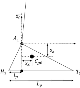
Figure 4: Detail of the foot parameters
3. The knee movement reproduces that of humans thus the knees do not bend backwards. We obtain two new conditions which are Ψ4 = q2−
q1 > 0 and Ψ5 = q3− q4 > 0.
4. The non-penetration of the mobile foot into the ground is verified by the two following conditions, which depend on the robot’s configuration: Ψ6 = zH2 > 0 and Ψ7 = zT 2 > 0 for the CK robot or Ψ6 = zH2′ > 0
and Ψ7 = zT 2′ > 0 for the RK robot.
The x-coordinates of the ZMP during the step is calculated with the equation:
xZM P = −Γ
1− (mpsxg)− (hpFLx)
FLz
(19) where mp represents the foot mass, sx is the x-coordinate of center of mass
of the foot (see Fig. 4) and Γ1, FLx, FLz are obtained with equation (8).
4. Parametrization of the gait
Several mathematical expressions are chosen as candidate function for the optimization. In this work, we use two mathematical functions for the trajectory angles:
• B´ezier functions.
• Cubic splines functions.
For each candidate function, the velocities and accelerations are obtained by successive derivation.
Every trajectory was developed to describe the evolution of absolute an-gles during a step of cyclic walk. The next step is symmetric with an exchange between the variables of thighs and shins (left leg takes the place of the right leg and vice versa). To simplify the calculations, the time t is normalized and described by tn= t/T where T is the period of the step. For tn = 0, the
left foot is on support and the right foot is behind the trunk. For tn = 1,
the right foot is advanced with a distance d and is in front of the trunk. The vector q = [q0, q1, q2, q3, q4, q5, q6]⊤represents absolute angles during the gait. The conditions of cyclicity for every configuration of gait are as follows:
• Foot soles are horizontal at the beginning and at the end of the step. • The angle of the fixed foot is equal to zero throughout the gait step
q0(tn) = 0.
• The trunk angle and the mobile foot angle functions are T-periodic. • The thighs and shins angle functions are 2-T periodic.
4.1. The B´ezier function
The first proposed candidate function is B´ezier function of order 3. They
are parametric trajectories where the curve is described with control points, i.e. we build a polygon with control points. The first and the last control points are the departure and the arrival of the trajectory. Other points serve to get a smooth trajectory by the determination of the centroid of the points. The trajectories of every joint are defined under the form below:
Bqi(tn) = 3 ∑ j=0 3! j!(3− j)!cijt j n(1− tn)(3−j) (20)
So, we have twenty four parameters to describe the evolution of the robot. The parameters ci0 and ci3 define the initial and final points respectively.
The parameters ci1 arise from impact conditions. Other parameters ci2 will
be found by optimization. The reduction of the number of parameters with the conditions of cyclicity gives:
• For the trunk: c60 = c63
• For the mobile foot: c50 = c53
• For the thighs: cij = ci(3−j), i = [2, 3], j = [0, 3]
• For the shins: cij = ci(3−j), i = [1, 4], j = [0, 3]
The impact implies conditions on the initial velocities of the robot bodies. We thus have:
• For the trunk: c61 = 3(c60 − c62) + δ6,
• For the mobile foot: c51 =−3c52+ δ5
• For the thighs: c21 = 3(c20 − c32) + δ2, c31 = 3(c30 − c22) + δ3
• For the shins: c11 = 3(c10 − c42) + δ1, c41 = 3(c40 − c12) + δ4
We finally obtain eleven parameters to define the evolution of a gait step which are the initial positions of shins, thighs and trunk and the control points of positions 2 of B´ezier function for every body.
4.2. The cubic splines function
In this case, the expressions of joint variables are defined on two half-period and described by the following equations:
0≤ tn≤ 12 → fqi(tn) = 3 ∑ j=0 aijt j n (21) 1 2 ≤ tn ≤ 1 → f ′ qi(tn) = 3 ∑ j=0 bij(1− tn) j (22)
where aj and bj, j = [0 . . . 3] represent the necessary coefficients to
parame-terize every angular trajectory.
An addition of conditions of cyclicity is necessary for the continuity be-tween both functions. They are detailed below:
• For the trunk: a60 = b60, a62 = b62, a63 = b63 =−
4 3a62
• For the mobile foot: a50 = b50 = 0, a52 = b52, a53 = b53 =−
4 3a52
• For the thighs: a20 = b30, a22 = b32 = a32+ 6(a30−a20), b23 =−6((a20− a30) + 4 3(a21− a22)), a30 = b20, a32 = b22 = a22 + 6(a20− a30), b33 =−6((a30 − a20) + 4 3(a31 − a32))
• For the shins: a10 = b40, a12 = b42 = a42 + 6(a40− a10), b13 =−6((a10 −
a40) + 4 3(a11− a12)), a40 = b10, a42 = b12 = a12 + 6(a10− a40), b43 =−6((a40 − a10) + 4 3(a41 − a42))
The impact imposes conditions on the initial velocities of the robot bodies. We thus have:
• For the trunk: a61 = b61 + δ6,
• For the mobile foot: a51 = b51 + δ5
• For the thighs: a21 = b31 + δ2, a31 = b21 + δ3
• For the shins: a11 = b41 + δ1, a41 = b11 + δ4
To define the evolution of the robot, forty eight parameters are required. With all the conditions of cyclicity mentioned above, the number of the parameters drops to seventeen. The remaining parameters are calculated from the initial angular positions of shins, thighs and trunk, the final speeds and the initial accelerations of each body.
Vectors that define the cubic splines and B´ezier functions can still be
reduced. The initial angular positions of each body can be calculated using the inverse kinematic model and the conditions of contact of the two feet with the ground. The Cartesian positions of the hip thus replace the initial values of the leg angles. The time T is a parameter added to every vector to find the optimal period for performing the walking step. Table 1 summarizes the number of parameters used in each case.
5. Simulations and results
The simulations were made with the geometrical and dynamical param-eters of the robot HYdRO¨ıd. This robot is 1.39 m tall for a weight around 45 kg. The optimization of the walking trajectories was realized by using the mathematical expressions of the joint variables developed in Section 4.
Table 1: Summary of the vectors of the parameters according to the type of trajectories
Joint trajectory Size of Vectors of
parameter vector parameters p
B´ezier function 11 xHi,zHi,c60,
cj2 for j ={1 . . . 6} ,T
Cubic Splines function 17 xHi,zHi,a60,T ,
bj1 and aj2 for j ={1 . . . 6}
The radii r1 and r2 are chosen identical and equal to 5 cm. The influence of trajectories on the optimization criterion, the angular evolution and the torques of the actuator will be shown in the following section. Then, a focus on the comparison of the energy criteria of both kinematics will be made.
The pre-design parameters of every body for the robot HYDRO¨ıD are expressed in Table 2. These values are derived from the CAD model of the robot.
Table 2: Parameters HYDRO¨ıD robot
Body Lengths Masses Inertia Positions
moments of CoM [m] [kg] [kg.m2] [m] Feet Lp = 0.207 0.678 0.001 sx = 0.0135 lp = 0.072 sz = 0.0321 hp = 0.064 Shin l1 = 0.392 2.188 0.028 0.1685 Thigh l2 = 0.392 5.025 0.068 0.1685 Trunk l5 = 0.543 29.27 0.815 0.1921
5.1. The gait with different trajectory functions
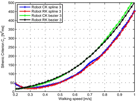
The evolution of the sthenic criterion with respect to the average walking speed is depicted as shown in Fig. 5. We observe in blue and green the optimal criterion for the robot with revolute joints and in red and black the optimal criterion for the robot with the rolling knee kinematics for the two types of functions described in Section 4. The results show that the criterion value of RK robot is lower than that of the CK robot. For the low speeds (between 0.1 and 0.26 m/s), trajectories described by the B´ezier functions
allow to obtain the best results during the walking for both robots. Cubic spline trajectories are the most adapted to describe the gait for the other speeds (greater than 0.26 m/s). The criterion mean value for the RK robot with the cubic spline functions is 7% lower than that for the CK robot. For example, for the RK robot, the minimum value of the criterion is 19 N2ms
obtained at the speed of 0.29 m/s. At this speed, the difference between the two criteria values is about 16%. Overall, whatever the type of function used to describe the gait, the RK robot consumes less energy.
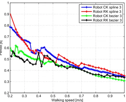
Fig. 6 and 7 present the evolution of the optimal periods of walking and the optimal step lengths depending on the walking speed resulting from the optimization. We notice that the periods for trajectories described by the
B´ezier function are lower than the ones for cubic spline functions.
Accord-ingly, step lengths are also shorter. We can thus say that robots make smaller steps more quickly by using the B´ezier trajectories. This promotes walking
at very low speeds thus the criterion is improved. We notice discontinuity in the period in the presented curves. So for criterion values that are quite sim-ilar, the periods may be very different, which appears in [28] with bifurcation modes.
The stick diagram (cf. Fig. 8) presents the evolution of the biped ac-cording to the kinematic used at the speed of 0.7 m/s by using cubic spline trajectories.
We can notice that whatever the configuration, the robot has the same gait of walking. The optimal speeds of walking found are close to results presented in [29] and [8]. The trunk bends slightly more forwards for the RK robot, unlike the CK robot. Fig. 9 shows the angular evolution of both configurations using B´ezier and cubic spline functions. The analysis of angles
for cubic spline trajectories confirms that the robot angles have the same shape for shins, thighs and trunk. Only the trajectory of the mobile foot for the RK configuration differs from the mobile foot for the CK configuration.
0.2 0.3 0.4 0.5 0.6 0.7 0.8 0.9 1 0 50 100 150 200 250 300 350 400 450 500 Walking speed [m/s] Sthenic Criterion C Γ [N 2 ms] Robot CK spline 3 Robot RK spline 3 Robot CK bezier 3 Robot RK bezier 3
Figure 5: The optimal sthenic criteria versus the walking speed for both robots and for each trajectory function.
The period for the RK robot is longer than that of the CK robot. For the
B´ezier trajectories, the shapes of the angular variables are identical.
Fig. 10 shows the evolution of joint torques for both configurations. The forms of the evolutions of the joint torques are in accordance with those quoted in the literature [8]. We notice that for both types of trajectories, the torques of the hips of the support leg and the mobile leg (Γ3 and Γ4) are lower for the RK configuration. The consequence is a knee torque slightly larger.
The analysis of the evolutions of the joint torques leads to the same selection of the actuators for the two configurations of robots. This means
0.2 0.3 0.4 0.5 0.6 0.7 0.8 0.9 1 0.2 0.3 0.4 0.5 0.6 0.7 0.8 0.9 1 Walking speed [m/s] Périod [s] Robot CK spline 3 Robot RK spline 3 Robot CK bezier 3 Robot RK bezier 3
Figure 6: Evolution of the period T in function of the walking speed for both robots and for each trajectory.
that for both knee configurations, motors and gearbox remain the same. In conclusion, the robot with rolling knee contacts will have greater autonomy.
5.2. Energetic comparison of the two configurations
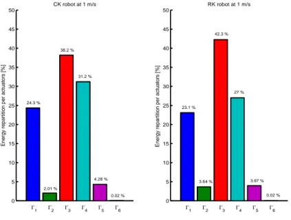
We are interested here in the distribution and the evolution of the cri-terion for each joint. The evolution of the joint torques allows the energy comparison joint by joint of both structures. The study was carried out for all the speeds. The trend of distribution being the same for the various speeds, only the results for the speed of 1 m/s are presented here. The equation to obtain this distribution is the following:
CΓi = 2 d ∫ T 0 Γ⊤i Γidt pour i = [1 . . . 6] (23) EnergyRatio = CΓi Cp (24)
0.2 0.3 0.4 0.5 0.6 0.7 0.8 0.9 1 0.2 0.3 0.4 0.5 0.6 0.7 0.8 Walking speed [m/s]
Length of the half−step [m]
Robot CK spline 3 Robot RK spline 3 Robot CK bezier 3 Robot RK bezier 3
Figure 7: Evolution of the step length in function of the walking speed for both robots and for each trajectory.
with Cp from equation (18).
Fig. 11 shows the distribution of the criterion for each joint for the speed of 1 m/s. We notice that the hip and the knee of support for the RK configuration use more energy than those of the CK configuration. The actuator of the mobile hip of the RK structure absorbs less energy. Fig. 12 shows that the various actuators have the same evolution during the phase of walking for both robots. The energy distribution for the mobile leg and the ankle of support for RK robot is lower compared to CK robot. Only the hip of support uses more energy for the RK robot.
6. Conclusion
The model of a new knee kinematic structure has been developed and compared with that of a robot having a structure with revolute joint on the knees. The study is made on two types of trajectory that are described with
−0.4 −0.2 0 0.2 0.4 0.6 −0.2 0 0.2 0.4 0.6 0.8 1 1.2 1.4 1.6 x[m] z[m] −0.4 −0.2 0 0.2 0.4 0.6 −0.2 0 0.2 0.4 0.6 0.8 1 1.2 1.4 1.6 x[m] z[m]
Figure 8: Stick diagram of the displacement of bipeds for the walking speed of 0.7 m/s. At left, the revolute configuration and at right, the rolling knee configuration. The green diamond represents the center of mass position. The plus marker represents the evolution of the ZMP position.
cubic spline or B´ezier functions. The results show that the new kinematics of
the knee reduces sthenic criterion by about 7% with cubic spline trajectories compared to the results obtained with the revolute joint structure. The decrease of this criterion is clearly visible on the graph of distribution (see Fig. 11).
The perspectives of our study will bring in various phases of walking as the double support and the modification of the geometrical parameters (radii
r1 and r2) which could be a way of improving energy gain. Thanks to the selection of actuators, the addition of the parameters of dry and viscous fric-tions in the dynamic model will allow to know the global energy consumption and the real advantage of the new knee kinematics.
Our future work concerns the study of trajectories with double support phase. To improve the energy efficiency of the robot, we propose to change the radii of the contact cylinders of the knees and/or to modify the shape
0 0.1 0.2 0.3 0.4 0.5 −0.4 −0.3 −0.2 −0.1 0 0.1 0.2 0.3 time [s] Angle [rad] CK Spline function at 0.7 m/s 0 0.1 0.2 0.3 0.4 0.5 −0.4 −0.3 −0.2 −0.1 0 0.1 0.2 0.3 time [s] Angle [rad] RK Spline function at 0.7 m/s 0 0.1 0.2 0.3 0.4 0.5 −0.4 −0.3 −0.2 −0.1 0 0.1 0.2 0.3 time [s] Angle [rad] CK Bezier function at 0.7 m/s 0 0.1 0.2 0.3 0.4 0.5 −0.4 −0.3 −0.2 −0.1 0 0.1 0.2 0.3 time [s] Angle [rad] RK Bezier function at 0.7 m/s q0 q1 q 2 q3 q4 q5 q6
Figure 9: Evolution of absolute joint an-gles for the walking speed of 0.7 m/s
0 0.1 0.2 0.3 0.4 0.5 −15 −10 −5 0 5 10 15 time [s] CK Spline function at 0.7 m/s Γ1 Γ2 Γ3 Γ4 Γ5 Γ6 0 0.1 0.2 0.3 0.4 0.5 −15 −10 −5 0 5 10 15 time [s] Torque [N.m] RK Spline function at 0.7 m/s 0 0.1 0.2 0.3 0.4 0.5 −15 −10 −5 0 5 10 15 time [s] CK Bezier function at 0.7 m/s 0 0.1 0.2 0.3 0.4 0.5 −15 −10 −5 0 5 10 15 time [s] Torque [N.m] RK Bezier function at 0.7 m/s
Figure 10: Evolution of joint torques for the walking speed of 0.7 m/s
0 5 10 15 20 25 30 35 40 45 50
Energy repartition per actuators [%]
CK robot at 1 m/s Γ1 Γ2 Γ3 Γ4 Γ5 Γ6 0 5 10 15 20 25 30 35 40 45 50
Energy repartition per actuators [%]
Γ1 Γ2 Γ3 Γ4 Γ5 Γ6 RK robot at 1 m/s 2,01 % 24.3 % 38.2 % 31.2 % 4.28 % 0.02 % 23.1 % 3.64 % 42.3 % 27 % 3.97 % 0.02 %
Figure 11: Distribution of criterion on the actuators for the walking speed of 1 m/s
of the contact surface of the knees. Using the results of joint torque and speed profiles, it is possible to select the actuators. Thus, models of friction, gearboxes and electrical losses can be determined. This leads naturally to
0 0.1 0.2 0.3 0.4 0 20 40 60 80 100 120 140 160 180 200 time [s] CΓ i [N 2.m.s] 0 0.1 0.2 0.3 0.4 0 20 40 60 80 100 120 140 160 180 200 time [s] CΓ i [N 2.m.s] CΓ 1 CΓ 2 CΓ 3 CΓ 4 CΓ 5 CΓ 6 CΓ 1 CΓ 2 CΓ 3 CΓ 4 CΓ 5 CΓ 6
Figure 12: Evolution of sthenic criterion on the actuators for the walking speed of 1 m/s
repeat the optimizations with an energy criterion to determine the overall transport cost of the robot.
7. Acknowledgement
The authors gratefully acknowledge the contribution of French National Research Agency for its financial support of A.N.R. ARPEGE program, project ANR-09-SEGI-011-R2A2.
References
[1] G. Van Oort, R. Carloni, D. Borgerink, S. Stramigioli, An energy effi-cient knee locking mechanism for a dynamically walking robot, in: Pro-ceedings - IEEE International Conference on Robotics and Automation, 2011, pp. 2003–2008.
[2] A. Hamon, Y. Aoustin, Cross four-bar linkage for the knees of a planar bipedal robot, in: 10th IEEE-RAS International Conference on Hu-manoid Robots, HuHu-manoids 2010, 2010, pp. 379–384.
[3] G. Gini, U. Scarfogliero, M. Folgheraiter, New joint design to create a more natural and efficient biped, Applied Bionics and Biomechanics 6 (1) (2009) 27–42.
[4] T. Howard, L. Berviller, P. Zattarin, G. Abba, Optimized design for the knee structure of a humanoid robot, in: ASME 2012 11th Biennial Conference on Engineering Systems Design and Analysis, ESDA 2012, Vol. 2, 2012, pp. 391–397.
[5] T. Schauß, M. Scheint, M. Sobotka, W. Seiberl, M. Buss, Effects of compliant ankles on bipedal locomotion, in: Proceedings - IEEE Inter-national Conference on Robotics and Automation, 2009, pp. 2761–2766. [6] M. Srinivasan, Fifteen observations on the structure of energy-minimizing gaits in many simple biped models, Journal of the Royal Society Interface 8 (54) (2011) 74–98.
[7] M. Scheint, M. Sobotka, M. Buss, Compliance in gait synthesis: Effects on energy and gait, in: 2008 8th IEEE-RAS International Conference on Humanoid Robots, Humanoids 2008, 2008, pp. 259–264.
[8] D. Tlalolini, C. Chevallereau, Y. Aoustin, Comparison of different gaits with rotation of the feet for a planar biped, Robotics and Autonomous Systems 57 (4) (2009) 371–383.
[9] R. Gregg, T. Bretl, M. Spong, Asymptotically stable gait primitives for planning dynamic bipedal locomotion in three dimensions, in: Pro-ceedings - IEEE International Conference on Robotics and Automation, 2010, pp. 1695–1702.
[10] S. Miossec, K. Yokoi, A. Kheddar, Development of a software for motion optimization of robots - application the kick motion of the HRP-2 robot, in: Proceedings of the IEEE International Conference on Robotics and Biomimetics, ROBIO 2006, Kunming, China, 2006, pp. 299–304.
[11] J. Rummel, Y. Blum, H. Moritz Maus, C. Rode, A. Seyfarth, Stable and robust walking with compliant legs, in: Proceedings - IEEE Inter-national Conference on Robotics and Automation, 2010, pp. 5250–5255.
[12] T.-Y. Wu, T.-J. Yeh, Optimal design and implementation of an energy-efficient, semi-active biped, in: Proceedings - IEEE International Con-ference on Robotics and Automation, 2008, pp. 1252–1257.
[13] S. Miossec, Contribution `a l’´etude de la marche d’un bip`ede, PhD thesis, ´
Ecole Centrale de Nantes, France, in french (November 27, 2004). [14] J. Bonnans, J. Gilbert, C. Lemarchal, C. Sagastizabal, Numerical
Opti-mization, 2nd Edition, 2006.
[15] C.-Y. Wang, W. Timoszyk, J. Bobrow, Payload maximization for open chained manipulators: Finding weightlifting motions for a puma 762 robot, IEEE Transactions on Robotics and Automation 17 (2) (2001) 218–224.
[16] G. Cabodevila, Determination of energy optimal gaits of biped robots, PhD thesis, University of Strasbourg, France, in french (January 15, 1997).
[17] J. C. Lagarias, J. A. Reeds, M. H. Wright, P. E. Wright, Convergence properties of the nelder-mead simplex method in low dimensions, SIAM J. Optim. 9 (1998) 112–147.
[18] K. McKinnon, Convergence of the nelder-mead simplex method to a non-stationary point, SIAM J Optimization 9 (1999) 148–158.
[19] J. Park, S. Lee, Generation of optimal trajectory for biped robots with knees stretched, in: Proceedings - IEEE International Conference on Robotics and Automation, 2009, pp. 166–171.
[20] M. Hobon, N. Lakbakbi Elyaaqoubi, G. Abba, Modeling of rolling knee biped robot, Technical Report RR6/2013-AG, ENSAM (October 2013). URL http://sam.ensam.eu/handle/10985/7480
[21] M. Spong, M. Vidyasagar, Robot dynamics and control, John Wiley and Sons, New-York, 1991.
[22] W. Khalil, E. Dombre, Modeling, identification and control of robots, Hermes Sciences Europe, 2002.
[23] R. M. Brach, Classical planar impact theory and the tip impact of a slender rod, International Journal of Impact Engineering 13 (1) (1993) 21 – 33.
[24] F. Pfeiffer, C. Glocker, Multibody Dynamics with Unilateral Contacts, Wiley, New York, 1996.
[25] W. Stronge, Planar impact of rough compliant bodies, International Journal of Impact Engineering 15 (4) (1994) 435 – 450.
[26] C. Chevallereau, G. Bessonnet, G. Abba, Y. Aoustin, Bipedal robots: modeling, design and building walking robots, ISTE and Wiley Editions, New York, 2009.
[27] Y. Hurmuzlu, F. G´enot, B. Brogliato, Modeling, stability and control of biped robots: a general framework, Automatica 40 (10) (2004) 1647 – 1664.
[28] B. Siciliano, O. Khatib (Eds.), Springer Handbook of Robotics, Springer, 2008.
[29] M. Rostami, G. Bessonnet, Sagittal gait of a biped robot during the single support phase. part 2: Optimal motion, Robotica 19 (3) (2001) 241–253.