is an open access repository that collects the work of Arts et Métiers Institute of Technology researchers and makes it freely available over the web where possible.
This is an author-deposited version published in: https://sam.ensam.eu Handle ID: .http://hdl.handle.net/10985/17729
To cite this version :
Taoufik QORIA, François GRUSON, Frédéric COLAS, Guillaume DENIS, Thibault PREVOST, Xavier GUILLAUD - Critical clearing time determination and enhancement of grid-forming converters embedding virtual impedance as current limitation algorithm - IEEE Journal of Emerging and Selected Topics in Power Electronics p.12 - 2019
Any correspondence concerning this service should be sent to the repository Administrator : archiveouverte@ensam.eu
is an open access repository that collects the work of Arts et Métiers ParisTech researchers and makes it freely available over the web where possible.
This is an author-deposited version published in: https://sam.ensam.eu Handle ID: .http://hdl.handle.net/null
To cite this version :
Taoufik QORIA, Francois GRUSON, Frederic COLAS, Guillaume DENIS, Thibault PREVOST, Xavier GUILLAUD - Critical clearing time determination and enhancement of grid-forming converters embedding virtual impedance as current limitation algorithm - IEEE Journal of Emerging and Selected Topics in Power Electronics p.1-1 - 2019
Any correspondence concerning this service should be sent to the repository Administrator : archiveouverte@ensam.eu
Abstract— The present paper deals with the post-fault
synchronization of a voltage source converter based on the droop control. In case of large disturbances on the grid, the current is limited via current limitation algorithms such as the virtual impedance. During the fault, the power converter internal frequency deviates resulting in a converter angle divergence. Thereby, the system may lose the synchronism after fault clearing and which may lead to instability. Hence, this paper proposes a theoretical approach to explain the dynamic behavior of the grid forming converter subject to a three phase bolted fault. A literal expression of the critical clearing time is defined. Due to the precise analysis of the phenomena, a simple algorithm can be derived to enhance the transient stability. It is based on adaptive gain included in the droop control. These objectives have been achieved with no external information and without switching from one control to the other. To prove the effectiveness of the developed control, experimental test cases have been performed in different faulted conditions.
Index Terms— Grid forming voltage source converter, virtual
impedance, current limitation, droop control, transient stability.
I. INTRODUCTION
rid-forming Voltage Source Converter (VSC) based on droop control [1] has been widely studied in Microgrid and uninterruptible power supply for several types of applications: stability analysis in islanding mode [2], active and reactive power sharing in parallel operation [3], [4], decoupling control of active and reactive power [5]). These studies have been recently extended to power transmission systems dominated by renewable energy sources [6] where new challenges appear such as power converter controllers tuning for stable operation in case of low switching frequency [7], [8], stability assessment for large power system [6],
This project has received funding from the European Union’s Horizon 2020 research and innovation program under grant agreement No 691800. This paper reflects only the author’s views and the European Commission is not responsible for any use that may be made of the information it contains.
T. Qoria, F. Gruson, F. Colas, and X. Guillaud are with Univ. Lille, Centrale Lille, Arts et Métiers Paris Tech, HEI, EA2697 - L2EP - Laboratoire d’Electrotechnique de Puissance, F-59000 Lille, France.
T. Prevost and G. denis are with Réseau de Transport d’Electricité (RTE), Versailles, France.
optimal placement of grid-forming converters in large power system [9].
Unlike grid-following converters that behave as current sources, grid-forming converters are very sensitive to external disturbances. Indeed, due to the voltage source behavior of a grid forming converter, the overcurrent protection deserve a specific attention [10]–[12]. Compared to synchronous generators (SGs) that can support up to seven times over its rated current, power converters can only cope with few percent of overcurrent 20% to 40%. Trying to mimic synchronous machine would require a very large oversizing of semiconductor components and induces large additional costs. Therefore, power converters have to be protected against extreme events as short circuits but also other events which may induce small overcurrent: phase shift, connection of large loads and tripping of a line [13].
Many control strategies have been proposed for grid-forming converter in order to limit the current during transients. One strategy is to limit the current with a saturated control algorithm. This control strategy has been implemented in different ways e.g.; [11], [14], [15]. Despite that the current saturation limits the current during transient; if no PLL is implemented, the voltage controller will not be able to keep the output AC voltage aligned with the grid one. Thereby, the system can become unstable during the post-fault phase [12]. Recently, innovative concepts based on Virtual Impedance (VI) [10], [12], [16]–[18] have been implemented to emulate the effect of a physical impedance when the current exceeds its nominal value. These methods have shown their effectiveness to limit the current transients in case of lines tripping [10] and heavy load connection [12] while keeping the same nature of the power source “i.e.; voltage source”. Moreover, they ensure more stability in comparison to the current saturation [12]. Hence, the virtual impedance control proposed in [12], [17] is adopted in this paper.
Conventionally, if a power converter loses the synchronism and becomes unstable after large disturbances, it will be disconnected from the main grid for safety purposes [19]. However, in future power systems dominated by renewable energy sources (RESs), grid-forming converters have not only to cope with current limitation, but also to feed loads and provide services to the main grid even after fault clearing. In the literature, some papers proposed to switch from voltage
Critical clearing time determination and
enhancement of grid-forming converters
embedding virtual impedance as current
limitation algorithm
Taoufik Qoria, François Gruson, Member, IEEE, Fréderic Colas, Member, IEEE, Guillaume Denis, Thibault Prevost, Xavier Guillaud, Member, IEEE,
control based on the droop control to the PLL-based current control [1], [20] in order to maintain the synchronism and to ensure a transient stability. These methods require a complex algorithm for fault detection, triggering conditions. Moreover, as specified by [1], fault recovery could only be achieved after a considerable retuning of the voltage controller and the power controller in order to avoid AC voltage collapse. Recently, the transient stability mechanism of the current source VSC based droop control has been discussed in the literature in [14], [21]–[23] in case of operating point change and a 50% voltage sag. However, to the best of our knowledge, the post-fault synchronization of the VSC based on droop control and virtual impedance operating as voltage source has not been discussed in the literature. Hence, the contributions of the present paper consist to:
- Explain theoretically the synchronization process of a VSC based on droop control and virtual impedance when it is subjected to large disturbances such as a three-phase bolted fault.
- Propose an adaptive droop control to increase the critical clearing time and to limit the angle variation during the fault, and thereby, to enhance the system dynamics and its transient stability after fault clearing.
This paper is mainly focused on a grid forming control with a negligible inertial effect, which allows to develop some simplified analytical expressions and to give some general considerations in term of transient stability analysis. Since the inertial effect can be modified by the control, it is also interesting to study the case when it is not negligible. Simplified approaches are not possible anymore, however, it is still possible to use the same methodology, thanks to the simulation results, to evaluate the transient stability and enhance the critical clearing time.
Contrary to the conventional methods where the control has to switch from one strategy to another one (e.g.; from droop control to PLL), or require a triggering condition to avoid a transient instability after fault clearing, the proposed control does not need to switch to other strategies during fault which simplifies its analysis.
To show the effectiveness of the developed control in ensuring a current limitation as well as stable post fault synchronization, an experimental test bench has been developed to validate the proposed control algorithm.
The reminder of this paper is organized as follow. Section II first describes the studied system and its control structure, then, it recalls the operation principle of the virtual impedance for current limitation and shows its impact on the system dynamics. Section III presents the synchronization process of
the grid-forming based droop control during and after fault clearing. Section IV proposes a variable droop control to enhance the transient stability of the power converter. Section V presents the developed experimental bench and the experimental validation of the proposed control.
II. GRID-FORMING VOLTAGE SOURCE CONVERTER BASED ON DROOP CONTROL AND VIRTUAL IMPEDANCE
A. Description of the system
The studied system is depicted in Fig. 1. It consists of a three-phase 2-Level VSC supplied by a DC voltage source. On the AC side, the VSC is connected to an AC grid through an 𝐿#𝐶#𝐿% filter. The AC grid is represented by an ideal AC
voltage source in series with its equivalent impedance (𝐿',𝑅' ).
In this paper, 𝑣, represents the modulated voltage by the
converter, 𝑖. the output current through the filter 𝐿#, 𝑒' the AC
voltage across the capacitor 𝐶#, 𝑖' the grid current through the
transformer inductance 𝐿%, 𝑣0%% the AC voltage at the point of
common coupling (PCC) and 𝑢2% the DC voltage.
Fig. 1. Power electronic converter connected to an AC system via an LCL filter.
B. Grid-forming control structure
Fig. 2 presents the grid-forming cascaded control structure. The control consists of an inner cascaded AC voltage and current loops represented in the synchronous rotating frame (SRF) [8]. The inner control is ensured by two cascaded proportional-integral controllers (PI), feedforward decoupling terms and compensations. The AC voltage loop determines the current reference to the current control, and generates the modulated voltage to the linearization stage that delivers the modulation signals to the switching stage of the power converter. The control angle 𝜃456 and the AC voltage
references 𝑒'∗78 are provided by a primary control based on the
droop control 𝑃 − 𝜔 and 𝑄 − 𝐸'.
The primary control is expressed by the following equations: 𝜔456− 𝜔.?@= 𝑚0𝜔CDDE EF.(𝑝 ∗− 𝑝 ,?.) (1) 𝑒'2∗ − 𝐸.?@ = 𝑛IJKLFML N.O 𝑞,?.− 𝑞 ∗Q (2)
𝜔C, 𝜔.?@, 𝜔456, 𝑚0 and 𝑛I are respectively the nominal
frequency in rad/s, the nominal grid frequency in per-unit, the internal frequency, the active and reactive droop gains. 𝜔% and
𝑇S denote the cut-off frequency and the time constant of the
low-pass filters in the active and reactive droops, respectively. The low-pass filter in the reactive power droop aims only to filter the measurement, while, its role on the active power droop is usually twofold: it is used to filter the measurement and also to provide inertia to the system.
For the active power droop, the low-pass filter can be placed on the active power measurement 𝑝,?., or on the error
between 𝑝,?. and 𝑝∗. However, the second possibility gives
an exact equivalence with the swing equation of the synchronous machine [24]. Moreover, it eliminates the zero of the closed loop transfer function of the active power [6].
C. Virtual impedance for current limitation 1) Recall on the virtual impedance principle
To cope with various kinds of events, a current limitation strategy has to be implemented. In this paper, the virtual impedance strategy for current limitation is adopted [12].
Fig. 3. Virtual impedance principle
As illustrated in Fig. 3, the VI operation principle is divided into three main phases:
- Overcurrent detection and activation (i.e.; Activation only when the current exceeds its nominal value 𝐼U= 1 p.u).
- Virtual impedance calculation. - AC voltage drop calculation.
The expressions of 𝑋4X, and 𝑅4X are given in (3a) and (3b).
𝑋4X= Y
𝑘 0[\]𝜎_/a𝛿𝐼 𝑖𝑓 𝛿𝐼 > 0
0 𝑖𝑓 𝛿𝐼 ≤ 0 (3a)
𝑅4X= 𝑋4X/𝜎_/a (3b)
where 𝛿𝐼 = 𝐼.− 𝐼U. 𝑘0[\] and 𝜎_/a are defined respectively
as the virtual impedance proportional gain and the virtual impedance ratio.
The parameter 𝑘0[\] is tuned to limit the current magnitude to
a suitable level 𝐼,jk during overcurrent in the steady state,
while 𝜎_/a ensures a good system dynamics during the
overcurrent. The tuning method of these parameters is explained in [12].
When the virtual impedance is activated, the new AC voltage references are given by (4) and (5):
𝑒'∗7= 𝑒'2∗l − 𝛿𝑒'7 (4)
𝑒'∗8= −𝛿𝑒'm (5)
where:
𝛿𝑒'2 = 𝑅4X𝑖.2− 𝑋4X𝑖.I (6)
𝛿𝑒'I = 𝑅4X𝑖.I+ 𝑋4X𝑖.2 (7)
2) Impact of the virtual impedance on the system dynamics
A simplified quasi-static model including the virtual impedance is derived with the following assumptions: - The inner control dynamics are neglected.
- The resistive effect is neglected since 𝑋 ≫ 𝑅.
The simplified model in Fig. 4 gathers actual electrical variables 𝐼' , 𝑉' and the AC voltage 𝐸' modified by the virtual
impedance 𝑋4X. In quasi static operation, it is possible to
calculate the active power with the classical formula:
𝑝,?.=
qr s 4r
_EF_rF_\]𝑠𝑖𝑛 (𝛿) (8)
𝛿 denotes the angle between the virtual VSC voltage 𝐸'l and
the grid AC voltage 𝑣'.
Fig. 4. Simplified quasi-static grid-forming model including VI
Assuming the angle 𝛿 is small, a second-order simplified system including the droop control is obtained as shown in Fig.5.
Fig. 5. Quasi-static model of the VSC based droop control
The closed loopexpression of the transfer function 𝑝 ∗/𝑝,?.
can be expressed as follow:
00∗ uvw= L LFxyEzyrzy\] u{|r s\r }.Fx yEzyrzy\] u{~E|r s\r}.• (9)
where the damping ratio 𝜁 and the natural frequency 𝜔U are:
𝜁 =L•‚ƒDE(_EF_rF_\])„
,{qr s4r , 𝜔U= …
ƒ,{DEqr s4r„
(_EF_rF_\]) (10)
The analytical formula (10) reveals the following information: - When 𝑋4X increases, the system becomes more damped (i.e.;
𝜁 increases) and slower (i.e.; 𝜔U decreases).
- When 𝑚0 decreases, the system is overdamped and slower.
These considerations will be used in the following sections. III. POST-FAULT SYNCHRONIZATION OF A GRID-FORMING
CONVERTER BASED DROOP CONTROL
Once the fault is cleared, the virtual impedance is disabled progressively. The power converter should be able to resynchronize to the AC grid only using local measurements. The aim of this section is to analyze the behavior in case of a large transient and to propose a method to enhance the transient stability of the grid-forming VSC based on the droop control. For the sake of simplicity, the 𝐿#𝐶# filter, the inner
control dynamics, and the reactive droop control are neglected in this section. The validity of these assumptions is cheeked in the next sections through time-domain simulations.
Some general trends are drawn from the simplified quasi-static model in Fig. 4. Different phases during and after the fault are explained with an increasing complexity i.e.; without and with VI, without and with inertia effect. Since these considerations are given on a very simplified model, some time-domain simulations are presented to check the trends obtained with the quasi static model.
A. Negligible inertial effect
The inertial effect is linked with the low-pass filter placed in the active power droop. This effect can be reduced so that it becomes negligible.
Based on the simplify model in Fig. 4, Fig. 6 depicts the synchronization process of the grid-forming converter subject to a three-phase bolted fault. In this first approach, the virtual impedance is not introduced (i.e. 𝑋4X = 0).
Fig. 6. 𝑝,?.(𝛿) diagram of a droop control based VSC with inertial effect For a given 𝑝∗, there are two equilibrium points (a) and (a’),
where the power 𝑝,?. is equal to its reference 𝑝∗. However,
only the equilibrium point (a) is stable from the perspective of small-disturbance analysis [25].
The initial angle 𝛿† is given by,
𝛿† = 𝑎𝑠𝑖𝑛 ˆ 0∗ ‰uŠ‹Œ (11) where 𝑃,jk= qrs4r _EF_r (12)
The maximum angle 𝛿,jk of the operation point a’ is
expressed as,
𝛿,jk = 𝜋 − δ† (13)
When a symmetrical three phase bolted fault occurs, 𝑝,?.
drops to zero. Since the filtering effect is neglected, the frequency deviates instantaneously,
ω‘’“= 𝑚0𝑝∗+ ω”•– (14)
Since 𝜔456 is higher than 𝜔' (Hyper-synchronism), the angle
increases (phase 1). When the fault is cleared, the voltage is supposed to recover instantaneously. The consequence is a straight vertical line from the operating point (b) to (c) (phase 2). During this phase 𝛿 = 𝛿%. 𝛿% denotes the clearing angle.
At the end of phase 2, 𝑝,?. is higher than 𝑝∗ leading
to 𝜔456< 𝜔' (Hypo-synchronism). It results in a decrease of
the angle from (c) to the equilibrium point (a) (phase 3). At the equilibrium point, 𝜔456= 𝜔' and 𝑝,?.= 𝑝∗.
The stability limit is reached when the clearing angle reaches 𝛿,jk. This specific angle is defined as the critical
clearing angle 𝛿%%. It can be concluded that when the inertial
effect is neglected, 𝛿%%= 𝛿,jk.
B. Non-negligible inertial effect
When the inertial effect is considered, the two first phases are unchanged. However, a new phase has to be introduced as shown in Fig. 7.
Fig. 7. 𝑝,?.(𝛿) diagram of a droop control based VSC with inertial effect Indeed, when the fault is cleared, 𝜔456 starts to decrease from
the value calculated in (14) following the low-pass filter dynamic. As long as 𝜔456> 𝜔', the angle keeps increasing
till 𝜔456= 𝜔' (phase 3). Once this condition is fulfilled, the
angle reaches its maximum value denoted 𝛿%l. Then, since
𝑝,?. is still higher than 𝑝∗, the frequency keeps decreasing,
which results in a decrease of the angle, and thereby, a movement of the operating point from (c’) to the equilibrium point (a) (phase 4). Once again, at the equilibrium point, 𝜔456= 𝜔' and 𝑝,?.= 𝑝∗.
When the inertial effect is considered, the stability limit is reached when 𝛿%l= 𝛿,jk. Hence, it can be concluded that the
critical clearing angle 𝛿%% is strictly lower than 𝛿,jk.
C. Introduction of the virtual impedance
The effect of the virtual impedance is now introduced to embed the current limitation in this analysis. Therefore, Fig. 6 is modified when the current exceeds its rated value.
(a)
(b)
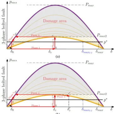
Fig. 8. 𝑝,?.(𝛿) diagram of a droop control based VSC and virtual impedance ,
The new expression of the maximum delivered active power including the virtual impedance is expressed as follow:
𝑃,jk•=
qrs4r
_EF_rF_\]uŠ‹ (15)
𝑋4XuŠ‹
is the virtual impedance defined from the current
limit 𝐼,jk.
Several 𝑝,?.(𝛿) may be drawn on Fig. 8.a for different values
of the virtual impedance comprised between 𝑋4X,jk and 0. The sequence of operations is now modified:
- Phase 1 is similar with or without virtual impedance. - Phase 2, the fault is cleared. As a consequence, the operating point moves first to (c), which is now located in the new curve 𝑝,?.= 𝑃,jk•𝑠𝑖𝑛 (𝛿).
- Phase 3, the operating point moves from (c) to (d). In this phase, 𝑋4X progressively decreases until 𝑋4X is equal to zero
(i.e.; when the operating point is equal to (d)).
- Phase 4, the virtual impedance is disabled and the operating point moves from (d) to the equilibrium point (a).
The activation of the virtual impedance results in a decrease of 𝑃,jk to 𝑃,jk• since the total impedance increases. As a
consequence, the system remains stable if the fault is cleared before 𝛿,jk4X expressed in (16).
𝛿,jk4X = 𝜋 − 𝑎𝑠𝑖𝑛 ˆ
0∗
‰uŠ‹•Œ (16)
Based on (16), a new stability limit is defined,
𝛿%% = 𝛿,jk4X (17)
As previously explained, in case where the inertial effect is not negligible, the angle keeps diverging till (c’) after the fault clearing, before recovering to the equilibrium point (a) (see Fig. 8.b). In this condition, a new stability limit is defined,
𝛿% ′ = 𝛿,jk4X (18)
Then 𝛿%%< 𝛿,jk\].
D. Critical clearing time calculation
Thanks to the previous considerations, it is now possible to calculate the critical clearing time, which is the maximum fault duration that guarantees the stability of the system. It is determined based on the critical clearing angle. The choice has been done in this paper to calculate the critical clearing time only when the inertial effect is neglected. Indeed, it allows obtaining a simple analytical formula from which it is possible to deduce the way to enhance the transient stability.
Since 𝑝,?. is equal to zero during the fault, the evolution of
the angle in time domain is given by the following equation, 𝛿(𝑡) = 𝑚0𝜔C𝑝∗𝑡 + 𝛿† (19)
The critical clearing time is obtained when 𝛿 reaches 𝛿%% ,
which is equal to 𝛿,jk\] as explained in the previous
subsection. It yields: 𝑡% =
[›œ•ž \]Ÿ›]
,{D¢0∗ (20)
(20) can be also written as follow:
𝑡% =
J£Ÿj.¤UK {∗
¥uŠ‹•OŸ¦”§¨K¥uŠ‹{∗ O Q
,{D¢0∗ (21)
E. Estimation of the critical clearing time from time-domain simulations
To validate the accuracy of the information found with the simplified modeling, time-domain simulations have been
carried out in Matlab/SimPowerSystem with the parameters listed in Table I.
TABLEI
SYSTEM AND CONTROL PARAMETERS
Symbol Value Symbol Value
Pn 1 GW mp 0.04 p.u. Cos𝜙 0.95 𝐸.?@ 1.p.u fn 50 Hz Rg 0.01 p.u. Uac 320 kV ph-ph Lg 0.1 p.u. Rf= Rc 0.005 p.u. 𝜔% 62.8 rad/s Lf= Lc 0.15 p.u. nq 0.25 p.u. Cf 0.066 p.u. 𝐼U 1 p.u. 𝑘𝑝a\] 0.3387 p.u. 𝐼,jk 1.2 p.u. 𝑘0% 𝜎_/a 0.73 p.u. 10 𝑘0ª 𝑘¤ª 0.52 p.u 1.16 p.u. 𝑘¤% 1.19 p.u. 𝑇S 31.8 ms A specific attention should be paid to the choice of 𝜔% (62.8
rad/s - 10 Hz). As previously mentioned, this filter has two functions:
- To filter the power measurement. - To bring inertial effect.
Therefore, the choice of the cut-off frequency 𝜔% is made in
such a way to keep filtering the active power measurement and to have a negligible inertial effect. This will be checked when analyzing simulation results.
Fig. 9 shows the time-domain simulation for fault duration of 154ms which corresponds to the stability limits found in simulation. This duration is close to the theoretical value of 𝑡%= 171𝑚𝑠.
Fig. 9. Dynamic behavior of the system subjected to a three phase bolted fault.
During the fault, the active power is null as expected, the AC voltage magnitude 𝐸' is not null due to the connection
inductance 𝑋%. Moreover, the evolution of the angle is nearly
linear as found in (19). After the fault, the active power recovers following the dynamics of the droop control and the virtual impedance as shown by (10). It can be noticed that the angle starts to decrease just after the fault clearing, which confirms that the inertial effect can be neglected.
The red curve in Fig. 10 presents the dynamic 𝑝,?.(𝛿) curve.
It is resulting from the time-domain simulations in Fig. 9. Compared to the qualitative curve in Fig. 8.a, it can be noticed from the dynamic 𝑝,?.(𝛿) that the general trend of the
evolution is confirmed. Indeed, the inertial effect can be neglected since the angle starts to decrease as soon as the fault is cleared.
Fig. 10. Dynamic 𝑝,?.(𝛿) curves obtained from time-domain simulations
with negligible inertial effect
Some differences are observed between the theoretical 𝑝,?.(𝛿) curve in Fig. 8.a and the dynamic one from Fig. 10.
They can be explained by the fact that:
- The virtual impedance used for dynamic simulations takes into account the resistive effect.
- The dynamic of the grid side that prevents the AC voltage to recover instantaneously.
Additional simulation is gathered in Fig. 11 with an inertial effect of H = 5s (equivalent to 𝜔% = 2.5 rad/s). Such a low
value of the cut-off frequency leads to a poor active power damping as proved by (10). To avoid this issue, a derivative action has been added to the power loop as explained in [26].
Fig. 11. Dynamic 𝑝,?.(𝛿) curves obtained from time-domain simulations
with considerable inertial effect H=5s
Compared to the qualitative curve in Fig. 8.b, it can be noticed from the red dynamic 𝑝,?.(𝛿) curve drawn in Fig. 11 that the
general trend of the evolution is confirmed, where the phases
described previously are clearly depicted.
To have more general trends, a comparison between the critical clearing times in Fig. 12 has been achieved between three models for large range of operating points:
- The theoretical model in (21) (Yellow curve).
- The dynamic model with negligible inertia (red curve). - The model with important inertia (H= 5s) (Blue curve). It can be noticed that the red and yellow curves in Fig. 11 are very close. Therefore, the information drawn from the theoretical model can be considered as valid. If the inertial effect is important, the theoretical model is not valid anymore as expected. While, based on the observed results, the inertia has a positive effect on the critical clearing time as it is well-known in the conventional power system [25].
Fig. 12. The theoretical approach compared to time-domain simulations
Focusing on a system with negligible inertia, (19) and (21) highlights the large impact of the droop gain 𝑚0 on the angle
evolution, and therefore, on the critical clearing time: By decreasing 𝑚0 during the fault, the critical clearing time
increases and the angle evolution decreases as well, therefore, the system keeps the synchronism for a longer fault duration and recovers to its equilibrium point faster after fault clearing. IV. VARIABLE DROOP CONTROL FOR TRANSIENT STABILITY
ENHANCEMENT
The previous section has highlighted the impact of the droop gain on the post-fault dynamics and the transient stability of the system. A question arises about the way to manage the evolution of 𝑚0. Two different solutions are proposed in this
section.
To increase the critical clearing time, 𝑚0 must be decreased.
The 1st solution proposes to decrease 𝑚
0 in respect to the
current magnitude. The 2nd solution proposes to decease 𝑚
0 in
respect the AC voltage magnitude resulting from the virtual impedance.
At the end of this section, the effect of 𝑚0 is illustrated when
the inertial effect is not negligible.
All the system and control dynamics neglected previously are considered in this section i.e., the 𝐿#𝐶# filter, the inner control
dynamics, and the reactive droop control.
A. 1st solution: Adaptive droop gain in respect to the current
magnitude
Intuitively, there is always a tendency to choose the current as criterion to vary the parameter mp. The aim of this section consists in showing the advantages and drawbacks of using this solution.
𝑚0 is defined by (22). 𝛼 can take two empirical values as
defined in (23). If the output current exceeds its rated value, 𝑚0 is equal to one-tenth of its nominal value. Once the fault is
cleared and the current returns to a safe value, the droop gain recovers to its initial value 𝑚0= 𝑚0†.
𝑚0= 𝛼𝑚0† (22)
𝛼 = ®1, 𝐼.≤ 1 p. u
0.1, 𝐼.> 1 p. u (23)
Fig. 13 illustrates the system behavior using the 1st solution.
For a given operating point 𝑝∗= 0.9 p.u, a 400ms fault is
applied on the system. Contrary to the conventional droop control, the variable droop control ensures a stable operation even if the fault duration is much longer than the critical clearing time computed in the previous section.
Fig. 13. Transient stability with and without variable droop control
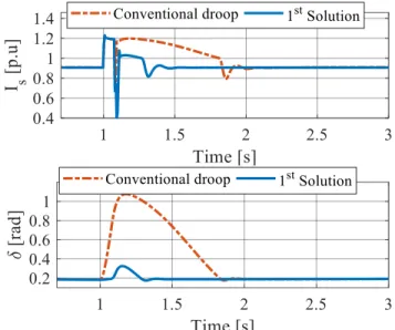
Decreasing 𝑚0 may have a second positive side effect.
In Fig. 14, the system behavior for a 75ms fault duration based on the conventional droop control (𝑚0 =𝑚0†) and the variable
droop control (𝑚0 =𝛼𝑚0†) is analyzed. With the conventional
droop control, the system needs around 800s to recover, whereas; with the variable droop control, the recovering time is around 300ms. In fact, when the droop gain decreases during the fault, the angle variation is limited as shown by (19), which explains the faster steady state recovery.
Fig. 14. Comparison of the system dynamic behavior for 75ms fault duration with constant or variable droop gain.
Nevertheless, the 1st solution may have a negative side effect
if the overcurrent occurrence is due to other kinds of events. To illustrate clearly its drawback, a phase shift of 30° is performed in Fig. 15 (In power transmission systems, the phase shift are especially linked to lines tripping). When a phase shift occurs, the current increase is limited by the virtual impedance, however, the current remains higher than 1p.u, as a consequence, the droop gain 𝑚0 remains frozen in 𝑚0=
𝛼𝑚0† which completely modifies the system dynamics as
proved by (10), therefore, the time to resynchronize is much longer than with the conventional droop control.
Fig. 15. The impact of the 1st solution on the system dynamics
B. 2nd Solution: Adaptive droop gain in respect with the AC
voltage amplitude
The AC voltage can be considered as a good indicator of the fault nature. In case of a short circuit, the voltage is decreasing and the droop control has to be decreased either. In case of a phase shift, the voltage amplitude remains nearly the same and the droop gain does not need to be modified. A solution could be to adjust the droop value with respect to the AC voltage level. The AC voltage can be considered as a good indicator of the fault nature. In case of a short circuit, the voltage is decreasing and the droop control has to be decreased either. In case of a phase shift, the voltage amplitude remains nearly the same and the droop value does not need to be modified. A solution could be to adjust the droop value with respect to the AC voltage level. However, it may lead to unwanted noises and fast transient variations. Therefore; a proposed solution consists in using the AC voltage reference, instead of the measured one. The adaptive droop gain is expressed as follow:
𝑚0= ‚𝑒'2∗•
+ 𝑒'I∗ •
𝑚0† (24)
(24) shows that the droop gain can be slightly modified in case of AC voltage reference change. To avoid this effect, (25) is introduced. Hence, the droop gain is modified only when the VI is activated.
𝑚0= ‚ƒ1 − δe³ ´„ •
During the fault, the droop gain is modified. It is possible to calculate the new droop gain in order to evaluate the new critical clearing time. During a three phase bolted fault at PCC
level, the droop gain is approximately equal to 𝑚0= 𝑍%𝐼,jk𝑚0 = 0.7%, which results in 𝑡%≈ 950 𝑚𝑠.
This value ensures a large stability margin compared to what is required by the present grid-code [19].
Such a small value of 𝑚0 cannot be maintained in normal
operation, because it would induce a large active power variation in case of small frequency fluctuations.
The time-domain simulations of the system are performed for a 400ms fault duration (Fig. 16) and a 30° phase shift (Fig. 17). A comparison is achieved between the first and the second solution based variable droop control.
Fig. 16. Dynamic comparison between the 1st and 2nd solution based variable
droop control in case of a 3-phase bolted fault.
Fig. 17. Dynamic comparison between the 1st and 2nd solution based variable
droop control in case 30° phase shift.
The obtained results show similar behavior in both solutions for a 3-phase bolted fault (Fig. 16). In case of a phase shift, the second solution reveals much better in terms of dynamic behavior (Fig. 17). Indeed, since the voltage is nearly constant, the droop gain is not modified so the dynamics of the system does not change too much. Therefore, it is possible to conclude that the 2nd solution is a generic solution that can
cope with various overcurrent situations.
In the following simulation, the same test cases in Fig. 16 and Fig. 17 are performed, where the proposed solution is applied to the system with an inertial effect of H = 5s. Simulation results are gathered in Fig. 18 and Fig.19, respectively.
Fig. 18. The impact of the 2nd solution on the high inertia system subjected to
a three phase bolted fault
Fig. 19. The impact of the 2nd solution on the high inertia system subjected to
a 30° phase shift.
As explained in the previous section, the system based on the conventional droop control with H=5s remains stable if the fault duration is 𝑡%≤ 230 ms for 𝑝∗= 0.9 p.u. In this context,
the simulation results draw interesting results: with or without inertia effect, the proposed solution shows it effectiveness to ensure a transient stability of the system for longer fault duration.
V. EXPERIMENTAL RESULTS
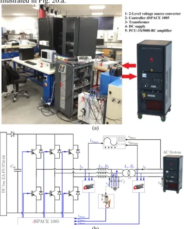
The aim of this section is to validate experimentally the theoretical developments. The experimental bench is illustrated in Fig. 20.a.
(a)
(b)
Fig. 20. The experimental bench. (a) Mockup presentation, (b) Functional schema
The 2-Level VSC (1) is supplied by an ideal and 600V DC voltage (4) source and connected to a high bandwidth AC amplifier (5) through an LCL filter (3) as presented in Fig. 20.b. The amplifier is used to emulate the AC system (i.e.; 300V ph-ph) as well as to generate the events discussed in this
paper (i.e.; a 100% voltage sag emulating a 3 phase bolted fault and a phase shift). The 2-Level VSC is controlled with a dSPACE DS1005 (2) with a 40 𝜇𝑠 time step. The switching frequency of the converter is 𝑓.¼= 10𝑘𝐻𝑧.
The electrical quantities displayed in experimentation are respectively the grid voltages 𝑣' in (𝑎𝑏𝑐) frame, the active
power 𝑝,?. and the internal frequency 𝜔456 as well as the AC
voltage amplitude across the capacitor 𝐸' and the VSC output
current 𝐼. in 𝑑 − 𝑞 frame.
The mockup parameters are listed in Table II.
TABLEII MOCKUP PARAMETERS Symbol Value Sn 5.625 kVA 𝐼U 10.8A fn 50 Hz Lf 10.9mH Lc 12.9mH Cf 9.2 𝜇F
A. Balanced three-phase bolted fault
At t=𝑡†, 𝑝∗= 0.7𝑝. 𝑢, then, a 200ms fault is applied. Fig. 21
shows the system dynamics based on the conventional droop control and Fig. 22 shows the system dynamics based on the adaptive droop control, i.e.; 2nd solution proposed in section
IV.
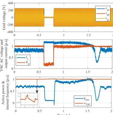
Fig. 21. System dynamics based on the conventional droop control
When the fault occurred, both strategies show that the AC voltage drop induces an increase of the VSC output current 𝐼.
which is limited to 1.2 p.u thanks to the virtual impedance. The active power is not equal to zero because of the resistive part of the system. During the fault, the frequency deviation is more important with the conventional droop control resulting in a slow recovering to the equilibrium point (around 1s) as shown in Fig. 21, while, the variable droop ensures a faster post-fault synchronization (around 250ms) as shown in
Fig. 22. The obtained results support the result obtained in the previous section in terms of dynamic improvement (Fig. 14).
Fig. 22. System dynamics enhancement based variable droop control
Fig. 23. Transient unstability phenomenon based conventional droop control
In the previous test case, the fault duration was less than the critical clearing time, in Fig. 23, a 250ms fault duration is applied to the system controlled with the converntionl droop control. During the fault the current is well limited to the desired value, however, after fault clearing, the system loses the synchonization and becomes unstable. The observed unstability phenomenon is nearly similar to what has been obtained in the previous section (Fig. 13). To show the effectivness of the variable droop control, a higher fault duration has been applied to the system (400ms) as depicted in Fig. 24, once the fault is cleared, the obtained results show that the system remains stable and reaches to its equilibrium point within 300ms.
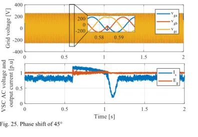
B. Phase shift
In this subsection, the power reference is first set to 𝑝∗= 0.7 p.u and a phase-shift of 45° is then applied as
illustrated in Fig. 25. The current rise to its maximum allowable value 𝐼,jk, then, the system reaches its equilibrium
point. The results obtained in Fig. 25 show the ability of the control to ensure a stable operation during a phase shift in addition to the short circuit.
Fig. 25. Phase shift of 45°
VI. CONCLUSION
In this paper, the synchronization of a grid forming converter based on droop control and virtual impedance is discussed when the system is subjected to large disturbances. Neglecting the inertial effect allows to derive a simple critical clearing time analytical formula which brings out the main influent parameters on the transient stability. A method to improve the stability limit and the dynamic behavior has been proposed. Comparisons between simulation and experimentation show that the proposed simplified model is relevant for the estimation of the critical clearing time and the understanding the general behavior during the resynchronization period. Even if the inertial effect has been analyzed qualitatively, the general trends will remain effective for a droop control with inertial effect. Some future works will be devoted to more general theoretical approach including this inertial effect in the study of the transient stability of grid-forming converters. In addition, the case of asymmetrical fault will also to be considered.
REFERENCES
[1] L. Zhang, L. Harnefors, and H. Nee, “Power-Synchronization Control of Grid-Connected Voltage-Source Converters,” IEEE Trans. Power
Syst., vol. 25, no. 2, pp. 809–820, May 2010.
[2] Y. A. I. Mohamed and E. F. El-Saadany, “Adaptive Decentralized Droop Controller to Preserve Power Sharing Stability of Paralleled Inverters in Distributed Generation Microgrids,” IEEE Trans. Power
Electron., vol. 23, no. 6, pp. 2806–2816, Nov. 2008.
[3] J. He and Y. W. Li, “An Enhanced Microgrid Load Demand Sharing Strategy,” IEEE Trans. Power Electron., vol. 27, no. 9, pp. 3984– 3995, Sep. 2012.
[4] H. Han, Y. Liu, Y. Sun, M. Su, and J. M. Guerrero, “An Improved Droop Control Strategy for Reactive Power Sharing in Islanded Microgrid,” IEEE Trans. Power Electron., vol. 30, no. 6, pp. 3133– 3141, Jun. 2015.
[5] Bin Li and Lin Zhou, “Power Decoupling Method Based on the Diagonal Compensating Matrix for VSG-Controlled Parallel Inverters in the Microgrid,” Energies, vol. 10, no. 12, p. 2159, Dec. 2017. [6] T. Qoria, Q. Cossart, C. Li, X. Guillaud, F. Gruson, and X. Kestelyn,
“Deliverable 3.2: Local control and simulation tools for large transmission systems,” p. 89.
[7] S. D’Arco, J. A. Suul, and O. B. Fosso, “Automatic Tuning of Cascaded Controllers for Power Converters Using Eigenvalue Parametric Sensitivities,” IEEE Trans. Ind. Appl., vol. 51, no. 2, pp. 1743–1753, Mar. 2015.
[8] T. Qoria, F. Gruson, F. Colas, X. Guillaud, M. Debry, and T. Prevost, “Tuning of Cascaded Controllers for Robust Grid-Forming Voltage Source Converter,” in 2018 Power Systems Computation Conference
(PSCC), 2018, pp. 1–7.
[9] B. K. Poolla, D. Groß, and F. Dörfler, “Placement and Implementation of Grid-Forming and Grid-Following Virtual Inertia and Fast Frequency Response,” IEEE Trans. Power Syst., pp. 1–1, 2019. [10] G. Denis, T. Prevost, M. Debry, F. Xavier, X. Guillaud, and A.
Menze, “The Migrate project: the challenges of operating a transmission grid with only inverter-based generation. A grid-forming control improvement with transient current-limiting control,” IET
Renew. Power Gener., vol. 12, no. 5, pp. 523–529, 2018.
[11] I. Sadeghkhani, M. E. Hamedani Golshan, J. M. Guerrero, and A. Mehrizi-Sani, “A Current Limiting Strategy to Improve Fault Ride-Through of Inverter Interfaced Autonomous Microgrids,” IEEE Trans.
Smart Grid, vol. 8, no. 5, pp. 2138–2148, Sep. 2017.
[12] A. D. Paquette and D. M. Divan, “Virtual Impedance Current Limiting for Inverters in Microgrids With Synchronous Generators,”
IEEE Trans. Ind. Appl., vol. 51, no. 2, pp. 1630–1638, Mar. 2015.
[13] G. Denis, “From grid-following to grid-forming: The new strategy to build 100 % power-electronics interfaced transmission system with enhanced transient behavior,” thesis, Ecole centrale de Lille, 2017. [14] M. Yu, W. Huang, N. Tai, X. Zheng, P. Wu, and W. Chen, “Transient
stability mechanism of grid-connected inverter-interfaced distributed generators using droop control strategy,” Appl. Energy, vol. 210, pp. 737–747, Jan. 2018.
[15] Q.-C. Zhong and G. C. Konstantopoulos, “Current-Limiting Droop Control of Grid-Connected Inverters,” IEEE Trans. Ind. Electron., vol. 64, no. 7, pp. 5963–5973, Jul. 2017.
[16] I. Erlich et al., “New Control of Wind Turbines Ensuring Stable and Secure Operation Following Islanding of Wind Farms,” IEEE Trans.
Energy Convers., vol. 32, no. 3, pp. 1263–1271, Sep. 2017.
[17] X. Lu, J. Wang, J. M. Guerrero, and D. Zhao, “Virtual-Impedance-Based Fault Current Limiters for Inverter Dominated AC Microgrids,”
IEEE Trans. Smart Grid, vol. 9, no. 3, pp. 1599–1612, May 2018.
[18] F. Salha, F. Colas, and X. Guillaud, “Virtual resistance principle for the overcurrent protection of PWM voltage source inverter,” in 2010
IEEE PES Innovative Smart Grid Technologies Conference Europe (ISGT Europe), Gothenburg, Sweden, 2010, pp. 1–6.
[19] “COMMISSION REGULATION (EU) 2016/ 631 - of 14 April 2016 - establishing a network code on requirements for grid connection of generators,” p. 68.
[20] K. O. Oureilidis and C. S. Demoulias, “A Fault Clearing Method in Converter-Dominated Microgrids With Conventional Protection Means,” IEEE Trans. Power Electron., vol. 31, no. 6, pp. 4628–4640, Jun. 2016.
[21] H. Xin, L. Huang, L. Zhang, Z. Wang, and J. Hu, “Synchronous Instability Mechanism of P-f Droop-Controlled Voltage Source
Converter Caused by Current Saturation,” IEEE Trans. Power Syst., vol. 31, no. 6, pp. 5206–5207, Nov. 2016.
[22] L. Huang, H. Xin, Z. Wang, L. Zhang, K. Wu, and J. Hu, “Transient Stability Analysis and Control Design of Droop-Controlled Voltage Source Converters Considering Current Limitation,” IEEE Trans.
Smart Grid, vol. 10, no. 1, pp. 578–591, Jan. 2019.
[23] L. Huang, L. Zhang, H. Xin, Z. Wang, and D. Gan, “Current limiting leads to virtual power angle synchronous instability of droop-controlled converters,” in 2016 IEEE Power and Energy Society
General Meeting (PESGM), 2016, pp. 1–5.
[24] J. Liu, Y. Miura, and T. Ise, “Comparison of Dynamic Characteristics Between Virtual Synchronous Generator and Droop Control in Inverter-Based Distributed Generators,” IEEE Trans. Power Electron., vol. 31, no. 5, pp. 3600–3611, May 2016.
[25] Kundur, Power System Stability And Control. McGraw-Hill, 1994. [26] T. Qoria, F. Gruson, F. Colas, G. Denis, T. Prevost, and X. Guillaud,
“Inertia effect and load sharing capability of grid forming converters connected to a transmission grid,” in 15th IET International
Conference on AC and DC Power Transmission (ACDC 2019), 2019,