THÈSE
En vue de l'obtention duDOCTORAT DE L’UNIVERSITÉ DE TOULOUSE
Délivré par l'Université Toulouse III - Paul SabatierDiscipline ou spécialité : Astrophysique
JURY
Dominique Toublanc (Président) Christian Jutten (Rapporteur)
Xander Tielens (Rapporteur) Javier Goicoechea (Examinateur)
Emilie Habart (Examinatrice) Christine Joblin (Directrice) Yannick Deville (co-Directeur)
Ecole doctorale : SDU2E Unité de recherche : CESR
Directeur(s) de Thèse : C. Joblin (CESR), Y. Deville (LATT) Présentée et soutenue par Olivier Berné
Le 03-10-2008
Titre : Evolution des très petites particules de poussière carbonée dans le cycle cosmique de la matière : méthodes de séparation aveugle de sources et spectro-imagerie avec le télescope spatial Spitzer
Universit´
e Toulouse III - Paul Sabatier
U.F.R Physique, Chimie, AutomatiqueTHESE
pour obtenir le grade de
Docteur de l’Universit´
e de Toulouse
d´
elivr´
e par l’Universit´
e Toulouse III - Paul Sabatier
Sp´ecialit´e
ASTROPHYSIQUE
pr´esent´ee au Centre d’Etude Spatiale des Rayonnements par
Olivier Bern´
e
´
Evolution des tr`es petites particules de poussi`ere carbon´ee dans le cycle cosmique de la mati`ere : m´ethodes de s´eparation aveugle de sources et
spectro-imagerie avec le t´elescope spatial Spitzer.
Soutenue le devant la commission d’examen D. Toublanc Pr´esident
A. Tielens Rapporteur
C. Jutten Rapporteur
J. Goicoechea Examinateur
E. Habart Examinatrice
C. Joblin Directrice de th`ese Y. Deville co-Directeur de th`ese
Remerciements
I wish to acknowledge the foreign collaborators I had the opportunity to work with during my stays abroad or in France, in particular Asunci´on Fuente who is at the OAN in Spain and Bill Reach who is at the California Institute of Technology (USA). I would like to thank Jehonghee Rho at Caltech for her interest in our work and help on super-nova remnants. I must thank J. D. Smith who is at the University of Arizona, for his help on the CUBISM software and IDL tips. I am indebted to Ryszard Szczerba at the N. Copernicus Astronomical Center in Poland for sharing his knowledge on planetary nebulae. I need to thank Javier Goicoechea at Ecole Normale Sup´erieure/Centro de Astrobiologia for leading this very nice project on propagation of star formation we both started two years ago. I am grateful to Achim Tappe at CfA in Harvard for nice scientifical and non-scientifical moments shared so as to Tomas Alonso in Madrid. Merci `a tous les collaborateurs qui m’ont aid´e dans mon exercice scientifique : Maryvonne Gerin (LERMA), Francois M´enard (LAOG), Alain Abergel (IAS), Estelle Bayet (UCL), Jean Charles Cuillandre (CFHT).
Merci au personnel du CESR et son directeur J. A. Sauvaud, aux directeurs successifs du d´epartement Univers Froid : Martin et Adam, merci aussi `a J.-P. pour les “IDL tips”, Isabelle pour ses encouragements, Claude pour sa bonne humeur, Aude et tout les autres du d´epartement.
Merci ´egalement aux gens du LATT en particulier Sylvie Roques, Herv´e Carfantan et Shahram Hosseini.
Je remercie sinc`erement Patrick Mascart de m’avoir autoris´e et encourag´e `a r´ealiser le projet d’illustration de mon manuscrit.
Je remercie ´egalement les membres de mon jury Xander Tielens, et Christian Jutten pour leurs nombreux conseils en tant que rapporteurs ; Javier Goicoechea et Emilie Habart pour leur relecture assidue de mon manuscrit et la pertinence de leurs com-mentaires en tant qu’examinateurs ; et M. le Pr´esident : Dominique Toublanc.
Je tiens a exprimer ma vive reconaissance envers mes directeurs de th`ese. Yannick Deville pour sa rigueur, son sens p´edagogique exemplaire et sa sympathie. Christine Joblin, pour sa disponibilit´e, pour son enthousiasme, la qualit´e de ses conseils, son engagement vis-`a-vis de ses e´tudiant, le respect de leur travail et son ´ecoute. Merci. Je remercie tout les jeunes du CESR et du LATT, avec prix special du jury `a Bap-tiste pour ses grosses roul´ees et Pierrick my ex-coloc. Special thanks `a Jonathan pour m’avoir offert de nombreuses Malborakis et Camelopoulos lors de notre trek dramatic en Cr`ete. Merci `a Nat’ pour sa gentillesse et sa bonne humeur quasi permanente, `a Ludo pour les quelques sessions zic et le prˆet de carte de cantine, `a Gilles pour les bons moments au festival d’astro, Lo¨ıc pour les discussions rugby... Merci `a Matthieu
4
et Johan au LATT pour le traitement du signal !
Merci `a Pauline le Guern pour son h´ebergement parisien qui `a contribu´e a la r´eussite de ce travail !
Merci `a Laure Cadars pour les illustrations qui donnent de la vie `a ce manuscrit. Je me dois de r´ediger une partie sp´ecialement r´eserv´ee `a mes amis Italiens. Grazie a : Giuliano, pour ton aide avec latex, tes pasta aux courgettes et au saucisson, tes nombreux nombreux conseils lors de mon intronisation dans le monde de la recherche et ton amit´ee. Roberta pour ton aide avec MIPS-SED et les pauses caf´es a CalTech. Giacomo pour ton aide sur de nombreux sujets reli´es ou pas `a l’astrophysique ! Valerio, pour les cigares et le Whisky `a l’Eb`ene et le cruizing dans la “chev’ cobalt” aux US. Francesca pour ta bonne humeur quotidienne qui a contribu´e `a faire du bureau 307 un lieu mythique. Paolo, pour les mˆemes raisons, et pour ton aide dans de nombreux calculs in-extremis de fin de th`ese et enfin Mauro pour ˆetre venu chaque jour nous rappeler qu’il faut aller manger.
Je remercie enfin tout ceux qui n’ont rien `a voir avec l’observation du firmament mais qui ont compt´es dans l’´elaboration de ce travail. Mes amis, et en particulier `a la fine ´equipe r´esidant au 9 Rue Antoine Darquier, tous les toulousains, et amis brestois qui m’ont soutenu pendant ces trois ans. Anna. Et enfin la famille Robin, Bonnet, Bern´e, Agn`es, les soeurs f´etides : ´Elise et Lulu, Mˆoman et J.-Y, M.-A. et Papa.
Contents
Introduction [en] 11
Introduction [fr] 13
I
Birth, life and death of stars: the cosmic cycle of matter 17
I.1 The cycle of matter in our galaxy 21
I.1.1 The cycle . . . 21
I.1.2 Gas and dust in the interstellar medium . . . 23
I.1.3 Lifecycle of cosmic dust . . . 23
I.1.4 Observing dust . . . 24
I.1.4.1 Extinction and emission of dust . . . 24
I.1.4.2 Infrared space astronomy . . . 25
I.1.4.3 The Spitzer space telescope . . . 26
I.2 Very small dust particles in the cosmic cycle 29 I.2.1 Spectral properties of very small dust particles in the Galaxy . . . . 29
I.2.1.1 Aromatic Infrared Bands . . . 29
I.2.1.2 Other spectral features related to carbonaceous material . 30 I.2.2 Formation, evolution and destruction of very small dust particles . 33 I.2.2.1 Formation in late carbon stars... . . 33
I.2.2.2 ...evolution in the diffuse ISM... . . 33
I.2.2.3 ...in molecular clouds... . . 33
I.2.2.4 ...during star formation,... . . 34
I.2.2.5 ...and destruction in supernovae and Hii regions. . . 34
I.2.2.6 In external galaxies and at high redshift . . . 34
I.2.3 Spectral variations of AIB emission . . . 34
I.2.3.1 In the cosmic cycle of dust . . . 34
I.2.3.2 Inside photodissociation regions . . . 35
I.2.3.3 Observations of AIB evolution with Spitzer . . . . 36 5
6 Contents
II
Unveiling the spectra of very small dust particles using
Blind Signal Separation methods
41
II.1 Blind signal separation methods 45
II.1.1 Introduction . . . 45
II.1.1.1 Independent component analysis . . . 46
II.1.1.2 Non negative matrix factorization . . . 47
II.1.1.3 Methods based on sparsity . . . 49
II.1.2 Blind signal separation in Astrophysics . . . 50
II.2 Testing BSS methods for the analysis of Spitzer spectro-imagery 53 II.2.1 Mid-IR dust emission: a linear instantaneous mixture BSS problem 53 II.2.2 Suitability of the mixing model for the application of BSS methods to Spitzer -IRS cubes . . . . 54
II.2.3 Tests on synthetic data . . . 54
II.2.4 Choice of the BSS method . . . 56
II.3 Disentangling the pure spectra of very small dust particles using NMF 59 II.3.1 Observations and data reduction . . . 59
II.3.1.1 Selected reflection nebulae . . . 59
II.3.1.2 Ced 201 . . . 60
II.3.1.3 The ρ-Ophiuchi filament . . . . 60
II.3.1.4 NGC 7023 East and North-West . . . 60
II.3.1.5 IRS observations and data reduction . . . 60
II.3.1.6 Zodiacal light . . . 63
II.3.2 Application to Spitzer data . . . . 63
II.3.3 Results . . . 65
II.3.3.1 Extracted spectra . . . 65
II.3.3.2 Efficiency of the reconstruction of the observations using the extracted spectra . . . 68
II.3.3.3 Spatial distributions of the extracted spectra . . . 68
II.3.4 Nature of the carriers of the extracted spectra . . . 78
II.3.4.1 Continuum-dominated spectrum . . . 79
II.3.4.2 Modelling the emission of VSGs versus BGs . . . 79
II.3.4.3 Pure band spectra: PAHs . . . 80
II.3.4.4 Ionization of PAHs in Ced 201, Oph-fil and NGC 7023-E 82 II.3.5 Evolution of the very small dust particles in the PDRs . . . 83
II.3.6 Conclusion . . . 84
II.4 Extended Red Emission of very small particles: from IR to visible 87 II.4.1 Visible observations . . . 87
II.4.2 BSS analysis . . . 89
Contents 7 II.4.4 Is the ERE carrier an important contributor to the mid-IR emission
spectrum ? . . . 94
II.4.5 Possible carriers of ERE in NGC 7023 . . . 94
II.4.5.1 The case of PAH++ . . . . 94
II.4.5.2 The case of [PAH2]+ . . . 95
II.4.6 Conclusion . . . 95
III
Following the emission of very small dust particles in
the cosmic cycle
97
III.1 A new basis to explain observed mid-IR spectra 101 III.1.1 The set of template spectra . . . 101III.1.1.1 Can we explain the emission of other astrophysical sources using the PDR extracted components ? . . . 102
III.1.1.2 The final basis . . . 105
III.1.1.3 Fitting procedure . . . 107
III.1.1.4 How good is the fit ? . . . 109
III.2 PNe: the processing of freshly made very small dust particles 111 III.2.1 Carbonaceous dust in planetary nebulae . . . 111
III.2.2 Observations and data reduction . . . 112
III.2.2.1 Observations . . . 112
III.2.2.2 Results . . . 114
III.2.3 Interpretation . . . 119
III.2.3.1 Grain processing . . . 119
III.2.3.2 PAH processing . . . 120
III.2.4 Conclusion . . . 124
III.3 Protoplanetary disks: from dust to planets 127 III.3.1 Introduction . . . 127
III.3.2 Observations and data reduction . . . 128
III.3.2.1 Selected sample . . . 128
III.3.2.2 Spitzer Observations . . . 129
III.3.2.3 ISO observations . . . 129
III.3.2.4 Characteristics of mid-IR emission from disks . . . 131
III.3.3 Results . . . 131
III.3.4 Probing disks with mid-IR emission ? . . . 131
III.3.4.1 The origin of the presence of the 8.3 µm broad feature . . 131
III.3.4.2 Processing of VSGs . . . 132
III.3.4.3 Evolution of PAH populations . . . 133
III.3.4.4 The mid-IR spectrum: a probe of the irradiation conditions of the disk . . . 136
8 Contents III.3.5 Putting new constraints on the nature of IRS 48 and Gomez’s
Ham-burger . . . 140
III.3.5.1 The luminosity of IRS 48 . . . 140
III.3.5.2 The nature of Gomez Hamburger . . . 140
III.3.6 Summary and conclusion . . . 141
IV
One step further: probing H ii regions and external
galaxies
143
IV.1 H ii regions : destroying very small dust particles ? 147 IV.1.1 The hard life of dust in H ii regions . . . 147IV.1.2 Improving our fitting technique . . . 148
IV.1.3 An example of UCH ii region: Mon R2 . . . 149
IV.1.3.1 The Mon R2 UCH ii region . . . 149
IV.1.3.2 Observations and analysis . . . 150
IV.1.3.3 Results and discussion . . . 150
IV.1.4 Conclusions . . . 154
IV.2 Nearby galaxies: carbonaceous dust at large scales in the ISM 155 IV.2.1 Nearby galaxies . . . 155
IV.2.1.1 The interest of studying nearby galaxies in the Mid-IR . . 155
IV.2.1.2 Observations and analysis . . . 156
IV.2.1.3 M82 . . . 156
IV.2.1.4 The Antennae merger (NGC 4038/39) . . . 158
IV.2.2 MIPS 8493: a distant luminous galaxy . . . 159
IV.2.3 Conclusions . . . 160
V
Summary and prospectives
161
V.1 Summary 163 V.1.1 A new picture of AIB emission in the ISM cycle . . . 163V.1.2 Probing astrophysical environments with AIB emission . . . 163
V.2 Prospectives 165 V.2.1 Towards a realistic photo-chemical and dynamical model for AIB emission . . . 165
V.2.2 The future of BSS methods... . . 166
Contents 9
Conclusion [en]
169
Conclusion [fr]
171
Appendices
175
Fine structure lines . . . 175
List of acronyms . . . 177 Publications . . . 179 Communications in conferences . . . 181
Bibliography
183
Abstract
197
R´
esum´
e
199
Introduction [en]
Amongst the people I meet randomly, many often ask a stunning question to me when we get to talk about our professions: what is the use of astronomy? Of course this question may seem legitimate, because one could think that we should rather save our efforts and huge amounts of money injected in space mission to solve issues that are more urgent than to know the origin of the universe. So how can we answer?
After many years struggling to find the best arguments, I must admit that I still have not reached a conclusion apart from the fact there is no concise answer to this question. Some will say that it is needed for long term evolution of mankind, and dare to point that what we learn from astronomy today will be useful in the future for hypothetical interstellar journeys... Some are more pragmatic, and would answer: “well CCDs which are now used in all the digital cameras were developed for and by astronomers”... Others prefer a more fundamental meaning to justify the role of astronomy: we need to know where we come from, where we live, and where we are going. Knowledge is a need for mankind as eating, and some of us should spend their time in expanding Knowledge. When I decided to be an Astronomer, it was, and still is, this last goal that motivated me, together with an outrageous need to satisfy an endless curiosity.
Somehow, this took me to study the tiny dust particles that are the ashes of sputtered off stars. More specifically, I focused on the extremely small (nano-metric) carbon based particles found everywhere in our galaxy, as a well as in other galaxies of the local and distant universe. They are formed in the envelopes of dying stars and injected into interstellar space. Under the effect of gravitation, the diffuse matter gathers into clouds and collapses giving birth to new stars. The disks that form around these young stars contains the building blocks of planets, including these carbonaceous particles. But except the fact that they are carbon based and small, little is known about their nature, or how they evolve during their life in the cosmic cycle.
Of course, in astronomy, only precise observations can provide the needed information to achieve such a work. In my case infrared observations are the key to understanding these tiny grains. This is because they absorb much of the UV light produced by stars and re-emit it in the infrared (IR). In fact, because of their small size these grains are heated to high temperatures (a few hundred K) after the absorption of a single UV photon and they thus re-radiate in the near to mid-IR (∼ 3-40 µm). Using modern space or ground based IR telescopes it is possible to directly observe their spectrum.
12 Introduction [en] What astronomers discovered is that the shape of these spectra varies strongly de-pending on the observed source and sometimes even inside a source dede-pending on the position. Though it is now clear that this is due to a modification of the nature of the emitting populations of particles it is still unclear what these populations are and how these modifications are linked to the local physical conditions, in particular the UV radiation produced by young massive stars. The goal of my PhD was to analyze the mid-IR emission spectrum of very small carbonaceous dust particles in a wide variety of astrophysical sources using observations from the recently launched Spitzer Space Telescope (NASA), in order to provide new insights into these questions: Why is the mid-IR spectrum of carbonaceous dust particles so different from a source to another? Are these differences linked to the local physical conditions? If they are, can we then use mid-infrared spectra to derive some information on the physical conditions of as-trophysical objects? How do the dust particles evolve in the cosmic cycle of matter?
The idea defended in this thesis is that the use of signal processing algorithms in par-ticular Blind Signal Separation algorithms (BSS), can help in addressing the above questions. This idea was first initiated in Christine’s group in particular with my pre-decessor Mathias who achieved a pioneering work, by providing a subtle mathematical decomposition of Infrared Space Observatory data. In this manuscript, I go several steps further following their work and adopting the hereunder detailed strategy. In the first Part of this thesis, I describe the cosmic cycle of matter and the evolution of very small dust particles inside this cycle. I also provide some evidence of the observed strong variations in the mid-IR emission spectrum of these particles, depending on the environment where they are observed. In the following part, I first give an overview of the main families of BSS methods, then test some of these methods to assess their efficiency for an application to Spitzer data, and finally apply them to real data ob-tained as part of our Spitzer observation program and some visible archival data from the Hubble Space Telescope and Canada France Hawaii Telescope. I discuss the new results which have been obtained and show how they fit into a chemical scenario in which polycyclic aromatic hydrocarbons (the PAH macromolecules which are also the smallest population of very small dust particles) are produced by evaporation of very small grains. Based on the successful results obtained, I present in part III a new method to analyze the mid-IR spectra of planetary nebulae and protoplanetary disks. In part IV, I go one step further and argue that the method presented for planetary nebulae and protoplanetary disks can be extended to regions of massive star formation (H ii regions) and external galaxies possibly even those situated in the distant universe. Finally I summarize the obtained results and present the main perspectives in terms of astrophysics/astrochemistry and signal processing methods following my work.
Introduction [fr]
Lors de mes rencontres al´eatoires avec les gens il arrive souvent que certains me posent cette question ´edifiante: quelle est l’utilit´e de l’astronomie ? Bien sˆur cette question peut sembler l´egitime, car finalement on peut se dire qu’il vaut mieux ´economiser nos forces, et les sommes colossales engag´ees dans les missions spatiales, pour traiter des probl`emes plus urgents. Alors comment r´epondre `a cette question ?
Je suis h´elas bien oblig´e d’admettre que je n’ai pas de r´eponse d´efinitive `a ce sujet, mis `a part le fait qu’il n’y a probablement pas de r´eponse concise. Certains, proba-blement les plus rˆeveurs, diront que ces recherches sont n´ecessaires car elles pr´eparent `a l’´evolution de l’esp`ece humaine `a long terme et `a d’hypoth´etiques voyages inter-stellaires... D’autres, plus pragmatiques, pr´ef´ereront invoquer l’utilit´e pratique: “Et bien, les CCD qui sont dans tout nos appareils photos num´eriques ont initialement ´et´e d´evelopp´es pour et par des astronomes !”... Enfin il y a ceux qui pr´ef`erent invoquer une raison plus profonde : nous avons besoin de savoir d’o`u nous venons, o`u nous vivons, et o`u nous allons. La Connaissance est essentielle `a l’existence humaine tout comme le besoin de se nourrir, et certains d’entre nous doivent donc s’attacher `a agrandir cette Connaissance. Je pense que c’est cette derni`ere raison qui m’a pouss´e `a devenir astronome ainsi qu’un besoin constant de combler ma curiosit´e.
Peut-ˆetre curieusement, ceci m’a amen´e `a ´etudier les petites particules de poussi`ere qui sont les cendres des ´etoiles ´eteintes. Je me suis plus particuli`erement int´eress´e aux particules carbon´ees extrˆemement petites (nano-m´etriques) qui sont omnipr´esentes dans notre galaxie et les galaxies ext´erieures, y compris celles de l’univers lointain. Elle se forment dans les enveloppes d’´etoiles en fin de vie et sont ensuite inject´ees dans l’espace interstellaire. Sous l’effet de la gravit´e, la mati`ere va peu `a peu se densifier pour former des nuages dont l’effondrement va donner naissance `a de nouvelles ´etoiles. C’est au sein des disques qui entourent ces ´etoiles jeunes que se forment les plan`etes y compris `a partir de ces minuscules poussi`eres. Certains pensent mˆeme que ces derni`eres peuvent avoir jou´e un rˆole dans la chimie pr´ebiotique qui donna ensuite naissance `a la vie. Mais mis `a part le fait que ces poussi`eres sont petites et faites de carbone on ne sait pas grand chose d’elles, ni sur leur nature exacte, ni sur la mani`ere dont elles ´evoluent dans le cycle cosmique de la mati`ere.
Bien sˆur, en astronomie, il n’y a pas de science sans observations de qualit´e. Dans mon cas il s’agit d’observations dans l’infrarouge (IR). En effet, ces toutes petites particules ont la propri´et´e d’absorber la lumi`ere ultra-violette (UV) produite par les ´etoiles pour
14 Introduction [fr] la re-´emettre dans l’IR. En fait, ces particules sont si petites que l’absorption d’un seul photon UV va les chauffer jusqu’`a des temp´eratures ´elev´ees (quelques centaines de K) ce qui leur permettra de rayonner dans l’IR proche `a moyen (∼ 3-40 µm). Grˆace aux moyens modernes d’observation, au sol ou dans l’espace, il est possible d’observer directement leur spectre. Ce que les astronomes ont d´ecouvert c’est que la forme de ce spectre varie selon la source astrophysique consid´er´ee et mˆeme selon la position `a l’int´erieur d’une mˆeme source. Il est `a peu pr`es clair que ces variations sont dues `a la modification de la nature physico-chimique des populations ´emettrices. Ce qui est beaucoup moins clair, c’est la nature de ces populations et la mani`ere dont les modifi-cations physico-chimiques sont li´ees aux conditions physiques du milieu, en particulier au champ de rayonnement UV produit par les ´etoiles jeunes et massives. Le but de ma th`ese est d’analyser le spectre infrarouge des tr`es petites particules de poussi`ere car-bon´ee dans un grand nombre de sources astrophysiques diff´erentes en utilisant les obser-vations du t´elescope spatial Spitzer (NASA) pour r´epondre `a ces questions : pourquoi le spectre IR-moyen des tr`es petites poussi`eres est-il si diff´erent d’une source `a l’autre ? Comment ces variations sont elles li´ees aux conditions physiques du milieu ? Peut-on, r´eciproquement, utiliser le spectre IR observ´e d’objets astrophysiques pour en d´eduire les conditions physiques qui y r`egnent ? Comment ces particules ´evoluent-elles dans le cycle cosmique de la mati`ere ?
L’id´ee d´efendue dans cette th`ese est que l’utilisation de m´ethodes de traitement du signal, en particulier les algorithmes de s´eparation aveugle de sources peuvent aider `a r´epondre aux questions ci-dessus. Cette id´ee `a ´et´e initialement introduite par le groupe de Christine en particulier par mon pr´edecesseur Mathias dans un travail fondateur, qui utilisait pour la premi`ere fois une d´ecomposition math´ematique subtile des observations du satellite ISO (Infrared Space Observatory). Je pr´esente dans ce manuscrit un certain nombre d’´evolutions, suite `a leur travail et en adoptant la strat´egie d´etaill´ee ci-dessous.
Dans la premi`ere partie de cette th`ese, je pr´esente le cycle de la mati`ere cosmique et ce que l’on sait de l’´evolution des tr`es petites particules de poussi`ere dans ce cycle. Je pr´esente aussi les observations qui mettent en ´evidence les variations du spectre IR-moyen de ces particules suivant l’environnement consid´er´e. Dans la partie suivante, je pr´esente les grandes familles de m´ethodes de s´eparation de sources puis en teste certaines pour confirmer qu’elles sont adapt´ees `a l’´etude des donn´ees Spitzer, pour fi-nalement les appliquer `a des donn´ees r´eelles obtenues dans le cadre de nos programmes d’observation avec Spitzer et `a des images d’archive du domaine visible obtenues avec le t´elescope spatial Hubble et au Canada France Hawaii Telescope. Je discute les r´esultats obtenus dans le cadre d’un sch´ema d’´evolution physico-chimique o`u les hydrocarbures aromatiques polycycliques (ces macromol´ecules PAH qui ont ´et´e propos´ees comme ´etant les plus petites des poussi`eres interstellaires) sont produites par ´evaporation des tr`es petits grains. Partant des r´esultats positifs obtenus, je pr´esente dans la partie III une nouvelle m´ethode pour analyser le spectre IR-moyen des n´ebuleuses plan´etaires et des disques protoplan´etaires. Je vais une ´etape plus loin encore dans la Partie IV, argu-mentant que cette m´ethode d’analyse peut s’´etendre `a l’´etude d’objets aussi complexes
Introduction [fr] 15 que les r´egions de formation d’´etoiles massives (r´egions H ii ) et les galaxies ext´erieures y compris, pourquoi pas celles situ´ees dans l’univers lointain. Enfin je r´esume mes r´esultats et pr´esente les perspectives possibles en astrophysique/astrochimie et traite-ment du signal suite `a mon travail.
Part I
Birth, life and death of stars: the
cosmic cycle of matter
“Dumb moon” by Laure Cadars, inspired by the first drawings of sky wonders by Galileo Galilei.
Chapter I.1
The cycle of matter in our galaxy
W
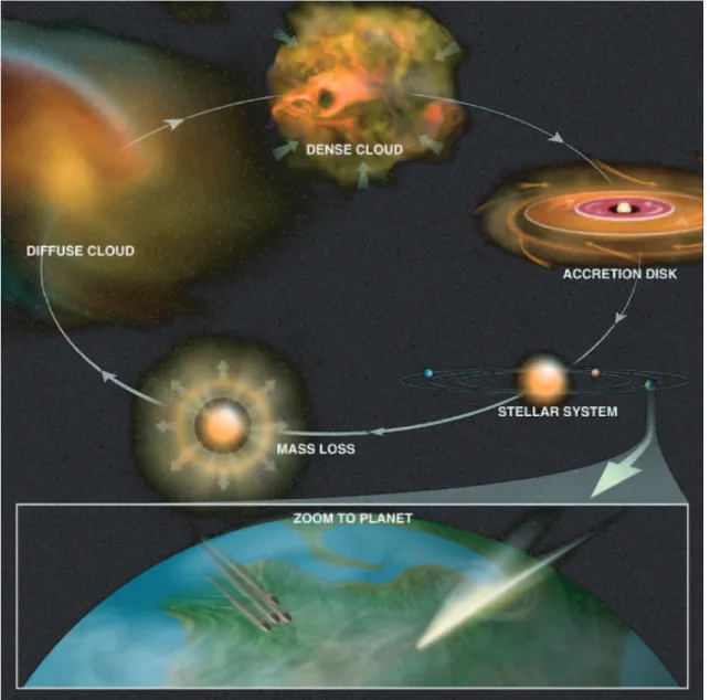
ith our bare eyes, in a clear night sky, we can see several thousands ofstars, all in our galaxy: the Milky Way. In fact, there are hundreds of billions of stars in the Milky Way (and there are hundreds of billions of galaxies in our universe). Seen from Earth, at our time scale, it may seem that starry skies are calm and static. This is of course an unrealistic picture of our universe where everything moves, interacts, collapses and dies along the steps of the cosmic cycle.I.1.1
The cycle
At the end of their lives, the most massive stars (M∗ > 10M¯) explode in supernovae.
Lighter stars including our Sun evolve to Asymptotic Giant Branch (AGB) stars. This phase is reached when stars have burnt their hydrogen supply completely, causing the core to contract and heat. This excess of heat causes the outer layers to expand and cool. The contraction of the central regions continues until the core reaches 100 million K igniting the fusion of Helium nuclei into Carbon and Oxygen. This fusion phenomenon is extremely unstable and will lead to huge pulsations, ejecting the star atmosphere into space. The remnants of atmosphere will create an envelope surround-ing the central pulsatsurround-ing star which will eventually ionize the ejected matter. After fusion of helium stops the star will finally cool down and become a white dwarf while the surrounding envelope keeps expanding into space. This is the planetary nebulae phase.
The gas and dust blown out from stars will accumulate to form diffuse clouds. Gravity will tend to gather all this matter, forming giant molecular clouds (GMC) that are much denser (10 to 1000 times). Some dense cores form in these clouds and become gravitationally unstable against collapse. A protostar will form, embedded
22 The cycle of matter in our galaxy
Figure I.1.1: Schematic view of the interstellar cycle of dust. CREDIT: Bill Saxton, NRAO/AUI/NSF
inside the cloud. During collapse, conservation of angular momentum combined with infall along the magnetic field lines leads to the formation of a rotating protoplanetary disk that drives the accretion process. At the same time, both mass and angular momentum are removed from the system by the onset of jets, collimated flows and the magnetic braking action. The resulting molecular outflow starts to erode and sweep up part of the natal envelope, contributing for the clearing of the circumstellar material and the termination of the infall phase.
The central core keeps on contracting, powering by the gravitational energy the luminosity of the young stellar object. It is in the T-Tauri (M∗ ≤ 2M¯ ) or Herbig
Ae/Be (2M¯ ≤ M∗ ≤ 8M¯ ) phase (more massive stars evolve so quickly that it is
I.1.2 Gas and dust in the interstellar medium 23 form out of it by accretion of debris. Eventually the star will contract enough and its core will heat up to temperatures allowing the ignition of Hydrogen fusion. It will be in the main sequence and live from several tens of million years (M∗ ∼ 8M¯) to 10
billion years (M∗ ∼ 1M¯) until they reach the AGB phase again.
I.1.2
Gas and dust in the interstellar medium
Our galaxy is largely empty as the star density is of about 6×10⁻²pc−3. What is
in between these stars is called the interstellar medium (ISM). It is this space that provides the medium to recycle matter in the cosmic cycle described above. It is mainly composed of hydrogen (70.4 % in mass) and helium (28.1 %) which was formed in the early universe. Heavier elements (C, N, O, Fe...) which compose only 1.5 % of the ISM were synthetized later in stars and injected in the ISM at their death. From these atoms, molecules can form and more than 140 of them have been detected so far1. The biggest components found in the ISM are dust grains, which contain a large
amount of the heavy elements.
I.1.3
Lifecycle of cosmic dust
Dust is formed at high densities and high temperatures in the envelopes of evolved stars (see Sect. III.2). Dust grains are mostly composed of silicates, graphite and amorphous carbonaceous dust, and carbides (Whittet 1992). During their lifetime in the cosmic cycle they undergoes strong shocks from supernovae explosions which will process or even destroy them (Jones et al. 1994, 1996). In denser regions, gas phase species will attach to these dust grains, either under the effect of Van Der Vaals forces (physisorption) or chemical forces (chemisorption). Dust grains are thought to play a fundamental role in the formation of molecules, in particular the most abundant one: H2. Atoms and molecules stuck at the surface of grains can migrate and meet to form
new molecules that can later be released under the effect of UV photons (Tielens and Hagen 1982). In cold molecular clouds, the accretion process will lead to the formation of ice mantles of e.g. CO2, H2O at the surface of grains. These ices can then be altered
by the effect of UV photons or cosmic rays leading to a complex photochemistry. Dust grains can also coagulate thus increasing the grain size. If not destroyed by shocks in the diffuse ISM, the same dust grain that was formed in the envelope of a dying star will eventually be incorporated in the protoplanetary disk of a newly formed star. Once inside the protoplanetary disk it will again undergo consequent processing before it is incorporated into planetary bodies. Thus, it is likely that the grains we find in our solar system, the matter in comets or meteorites, has been highly modified during the early phases of the Solar System. The idea that such bodies are a direct heritage of stardust is now more and more controverted, including taking into account the recent results from the STARDUST mission (see article and reports of special issue of Science published Dec 15, 2006).
24 The cycle of matter in our galaxy
Figure I.1.2: Left: The galactic center of the Milky Way seen in visible. A large fraction of the light emitted by stars is absorbed by dust which creates a dark shadow. Right: The extinction spectrum of the Milky way in the UV-Visible, with a model of the contribution of each dust component (From D´esert et al. 1990).
I.1.4
Observing dust
I.1.4.1
Extinction and emission of dust
Dust has the property to absorb and scatter UV-Visible photons produced by stars and is thus the dominant source of opacity in our galaxy (Fig. I.1.2). The absorbed energy is converted into thermal energy inside the grains and re-emitted in the infrared (IR). The IR photons can travel more freely than UV visible photons in the ISM since they are not absorbed efficiently by dust. Therefore these IR photons can easily be detected by telescopes, if it was not for the Earth atmosphere that absorbs IR photons. Therefore space telescopes have been used to probe the universe in the IR (see next section). We now have a complete picture of the IR spectrum of our own galaxy (Fig. I.1.3). Three major components are invoked in the model of D´esert et al. (1990) to explain the observed extinction and emission spectra:
• Big Grains (BGs): Large (& 0.1µm) silicate grains which dominate the far-IR to sub-millimeter emission in our galaxy. These grains are at thermal equilibrium with the interstellar radiation field (ISRF) and thus emit like a modified black body (E(λ) = λ−β × B(λ, T ), where B(λ, T ) is the black body function and β
the spectra index). They produce the λ−1 dependency of the extinction in the
UV-visible.
• Very Small Grains (VSGs): Stochastically heated (see Sect. I.2.1.1) carbon-based nanoparticles, proposed to explain the continuum emission between 20 and 80 µm and the UV bump in the extinction curve (Fig. I.1.2).
I.1.4 Observing dust 25
PAH
VSG
BG
?
Figure I.1.3: Left: The galactic center of the Milky Way seen in IR. The light absorbed by dust in the UV-visible is re-emmited in the infrared which unveils the structure of this region. Right: The emission spectrum of the Milky way in the IR, with the contribution of each dust components, following the D´esert et al. (1990) model. (J.-P. Bernard private communication)
• Polycyclic Aromatic Hydrocarbons (PAHs): Large aromatic molecules composed of carbon rings saturated with hydrogen atoms (Fig. I.2.1). They are stochasti-cally heated and responsible for the band emission in the mid-IR emission spec-trum of the Galaxy. They are believed to produce the so called far-UV rise in the extinction curve (Fig. I.1.2). Note that an extra continuum peaking at 2-3 µm is necessary to explain the observed emission. This emission originally detected by Sellgren (1984) in reflection nebulae is largely present in the diffuse medium of our galaxy (Flagey et al. 2006). Its origin is a complete puzzle as the carrier should be at the same time small to be hot enough to emit at 2-3µm (1000 K) and somewhat large to produce a continuum...
I.1.4.2
Infrared space astronomy
The infrared sky remained unexplored for a long time because most wavelengths in this range cannot be observed from the ground due to strong absorption bands in the Earth’s atmosphere. At the end of the seventies, the Kuiper Airborne Observatory (KAO) was the first observatory able to partly overcome this issue. A 90 cm telescope and IR instruments were mounted on a C-141 jet aircraft flying at 14 km of altitude, therefore getting rid of most of the absorption bands created by water vapour in the IR. In 1983 the first infrared satellite dedicated to astronomy was launched by NASA. It mapped nearly the whole sky at 12, 25, 60 and 100 µm and discovered over 500 000 infrared sources. The infrared astronomy revolution was brought in the 90s with the Infrared Space Observatory (Kessler et al. 1996), which included spectroscopy in the mid- to far-infrared. This mission lead to a number of discoveries. In 2003, the Spitzer Space Telescope (Werner et al. 2004, hereafter Spitzer ) was launched providing an unprecedented angular resolution and sensitivity in IR spectroscopy and imaging.
26 The cycle of matter in our galaxy
I.1.4.3
The Spitzer space telescope
Figure I.1.4: The Spitzer Space Telescope c°NASA/JPL/CALTECH
Spitzer (Fig. I.1.4) is an infrared satellite part of NASA’s great observatories, launched in 2003 and placed in an earth trailing heliocentric orbit. This spacecraft consists of a 0.85 meter telescope and three cryogenically-cooled instruments: the in-frared spectrograph (IRS), the inin-frared array camera (IRAC) and the multiband imag-ing photometer (MIPS).
I.1.4.3.1 The inrared spectrograph (IRS)
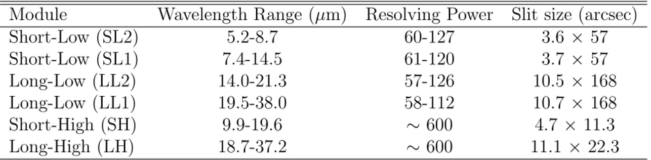
Most of the analyzes achieved during my PhD are based on data provided by the IRS. This spectrograph provides mid-IR slit spectroscopy in the 5.2 to 38.0 µm wavelength range. The IRS is composed of four separate modules, with two modules (SL and
I.1.4 Observing dust 27 LL for short low and long low respectively) providing a spectral resolution R = λ
∆ λ
of 60-120 over 5.2-38.0 µm and two modules (SH and LH short high and long high) providing R = 600 spectral resolution over 9.9-37.2 µm (see Table I.1.1). The SL and LL modules are divided into two submodules (SL1/2 and LL1/2).
Module Wavelength Range (µm) Resolving Power Slit size (arcsec)
Short-Low (SL2) 5.2-8.7 60-127 3.6 × 57 Short-Low (SL1) 7.4-14.5 61-120 3.7 × 57 Long-Low (LL2) 14.0-21.3 57-126 10.5 × 168 Long-Low (LL1) 19.5-38.0 58-112 10.7 × 168 Short-High (SH) 9.9-19.6 ∼ 600 4.7 × 11.3 Long-High (LH) 18.7-37.2 ∼ 600 11.1 × 22.3
Table I.1.1: Modules of the infrared spectrograph onboard Spitzer and their main characteristics
The IRS is a so-called slit spectrograph which provides imaging in one dimension along the slit. The angular dimensions of the slits for each modules are given in Ta-ble I.1.1. Moving the slit on the sky (spectral mapping mode) enaTa-bles to obtain 2D imaging as well as spectroscopy, leading 3D spectro-imagery with 2 spatial dimensions and one spectral dimension.
I.1.4.3.2 The infrared array camera (IRAC)
IRAC is a four-channel camera that provides simultaneous 5.2 x 5.2 arcminutes images at 3.6, 4.5, 5.8, and 8 µm. Two adjacent fields of view are imaged in pairs (3.6 and 5.8 µm; 4.5 and 8.0 µm) using dichroic beamsplitters. All four detector arrays in the camera are 256 x 256 pixels in size, with a pixel size of 1.2 x 1.2 arcsec in the plane of the sky. The two short wavelength channels use InSb detector arrays and the two longer wavelength channels use Si:As detectors.
I.1.4.3.3 The Multiband Imaging Photometer for Spitzer (MIPS)
MIPS provides the Spitzer Space Telescope with capabilities for imaging and pho-tometry in broad spectral bands centered nominally at 24, 70, and 160 µm, and for low-resolution spectroscopy between 55 and 95 µm. The instrument contains 3 sepa-rate detector arrays each of which resolves the telescope Airy disk with pixels of size lambda / 2D or smaller. All three arrays view the sky simultaneously; multiband imag-ing at a given point is provided via telescope motions. The 24 micron camera provides roughly a 5’ square field of view (FOV). The 70 micron camera was designed to have a 5’ square FOV, but a cabling problem compromised the outputs of half the array; the remaining side (“side A”) provides a FOV that is roughly 2.5’ by 5’. The 160 micron array projects to the equivalent of a 0.5’ by 5’ FOV and fills in a 2’ by 5’ image by multiple exposures. The 70 micron array also has a narrow FOV/higher magnification
28 The cycle of matter in our galaxy mode, and is additionally used in a spectroscopic mode.
Chapter I.2
Very small dust particles in the
cosmic cycle
W
e have seen in the previous chapter that the mid-IR spectrum of ourGalaxy is dominated by the emission of very small dust particles (basically PAHs and VSGs). In the following chapter we first present the main spectral features that characterize the emission and absorption of these particles. We then give an overview of what their life is in the cosmic cycle. Finally, we discuss on the possible origin of the observed variations of the mid-IR infrared spectral features.I.2.1
Spectral properties of very small dust
parti-cles in the Galaxy
I.2.1.1
Aromatic Infrared Bands
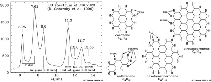
Aromatic Infrared Bands (AIBs) are relatively broad emission bands at 3.3, 6.2, 7.7, 8.6 11.3 and 12.7 µm seen throughout the Milky Way (Fig.I.2.1). There is a large consen-sus that the bands are due to the emission of Polycyclic Aromatic Hydrocarbons (see definition Sect. I.1.4.1 and schematic representation Fig. I.2.1) as proposed by L´eger and Puget (1984) and Allamandola et al. (1985). The AIBs are observed in nearly any environment combining the presence of dust and UV photons: planetary nebulae, dif-fuse ISM, Hii regions, reflection nebulae, protoplanetary disks, and external galaxies. PAH molecules absorb UV-visible photons of stars and re-radiate the absorbed energy in the IR. The heating mechanism of the AIB carriers was first proposed by Sellgren (1984). In this “stochastic heating” model (Fig. I.2.2), the very small dust particles
30 Very small dust particles in the cosmic cycle have the time to cool down between the absorption of two photons contrary to larger grains which can be considered at thermal equilibrium. The AIBs were then assigned to PAH vibrational modes by L´eger and Puget (1984) and Allamandola et al. (1985) as follows:
• C-H stretching mode at 3.3 µm • C-C stretching mode at 6.2 µm • C-C stretching mode at 7.7 µm
• C-H in-plane bending mode at 8.6 µm
• C-H out-of-plane bending mode with wavelength depending on the number of neighbour H atoms:
– 11.3 µm for “solo” H (no adjacent H) – 12.0 µm for “duo” H (2 contiguous H) – 12.7 µm for “trio” H (3 contiguous H) – 13.55 µm for “quartet” H (4 contiguous H)
Though the idea that PAHs are responsible for the observed AIBs is widely accepted, the identification of a specific PAH in the ISM has not been possible yet. This is mainly because all PAHs produce emission bands in the mid-IR. Thus, the observed spectra likely result from the emission of a mixture of PAH molecules. Mulas et al. (2006b) showed that, in principle, it is possible to identify specific interstellar PAHs using the ro-vibrational emission bands that arise in the far-IR during the cooling cascade following UV excitation. The observation of these bands in the far-IR domain requires airborne and/or satellite instruments due to strong atmospheric absorption, and extremely high sensitivity. Performing such identifications will be one of the goals of the Herschel Space Observatory (HSO) and SOFIA (Stratospheric Observatory For Infrared Astronomy)
I.2.1.2
Other spectral features related to carbonaceous
mate-rial
Extended red emission
Extended red emission (ERE) is a broad emission band (FWHM > 100 nm) emission centered at ∼ 700 nm and detected in a number of dusty environments. It was first observed in the Red Rectangle proto-planetary nebula, and later detected in reflection nebulae (Witt and Boroson 1990), diffuse ISM (Gordon et al. 1998), and galaxies (Perrin et al. 1995; Pierini et al. 2002). Numerous carriers have been proposed for this emission without clear identification (see review of possible carriers in Witt et al. 2006). The possible link with the carriers of the Aromatic Infrared Bands has been discussed
I.2.1 Spectral properties of very small dust particles in the Galaxy 31
Figure I.2.1: Left: The AIB features detected in the reflection nebula NGC 7023 by Cesarsky et al. (1996) using ISO. Right: Schematic view of different PAH molecules showing the C-H out of plane vibrational sites on the edges of the hexagonal carbon rings. Figure from Draine (2003).
Figure I.2.2: The temperature of an interstellar grain heated by the interstellar radiation field of
our galaxy as a function of time. Four sizes of grains are considered from a = 200 ˚A to a = 25˚A and
their photon absorption rates τabs are calculated. The big grain stays at a constant low temperature
while the small one (typically a PAH) heats up to a high temperature and has the time to cool down before it absorbs another photon. Figure from Draine (2003)
32 Very small dust particles in the cosmic cycle by several authors. Both types of emission features, ERE and AIBs, were found to be relatively cospatial although not matching (Furton and Witt 1990), pointing to different but related materials for their carriers (Furton and Witt 1992). Recently, a detailed study of the spatial distribution of the ERE in the northern PDR of NGC 7023 has been performed by Witt et al. (2006) who concluded that the ERE mechanism is a two-step process involving the formation of the carrier and then the excitation of the luminescence, and proposed doubly-ionized Polycyclic Aromatic Hydrocarbons (PAHs) as plausible carriers. On the other hand, recent quantum chemistry calculations point to PAH dimers ([PAH2]+) as the carrier of ERE (Rhee et al. 2007). We will rediscuss
this assignment in Sect. II.4.5. Diffuse interstellar bands
The extinction curve of our Galaxy exhibits a large number of weak absorption bands in the 0.38-1.3 µm range (Herbig 1995). These Diffuse Interstellar Bands (DIBs) were discovered over 80 years ago but not a single one of them could be identified convinc-ingly. Because most of these bands are quite broad (FWHM > 0.1nm ) they cannot be due to small molecules. Here again PAH molecules are good candidates to account at least for some of these DIBs.
Figure I.2.3: Other spectral features attributed to carbonaceous dust and/or macromolecules, Left: Extended Red Emission (ERE) observed in the optical spectrum of NGC 7023 (from Gordon et al. 2000). Right: Diffuse interstellar bands (DIBs). Figure from Draine (2003) based on Jenniskens and Desert (1994).
I.2.2 Formation, evolution and destruction of very small dust particles 33
I.2.2
Formation, evolution and destruction of very
small dust particles
I.2.2.1
Formation in late carbon stars...
PAHs, as well as other carbon-based grains are likely formed in the envelopes of late carbon stars (see review by Kwok 2004) but the detailed mechanisms leading to their creation are not well understood yet. There is a wealth of theoretical studies suggesting that the pyrolysis of hydrocarbon molecules such as Acetylene (C2H2) can lead to the
formation of PAHs and eventually soot particles, in a chemical scheme close to the one occuring in combustion flames. Alternatively, Cernicharo et al. (2001) have suggested that photon-driven polymerization of acetylene could lead to the formation of benzene (C6H6), the smallest PAH. Note that even though it is believed that AGB stars harbor
the formation of carbonaceous dust there is no direct detection of the AIBs in AGB stars. This is most likely due to the fact that AGB stars are too cold to excite PAHs. However, their descendants i.e. (proto)planetary nebulae show strong AIB emission (Kwok 2004).
I.2.2.2
...evolution in the diffuse ISM...
Once formed, PAHs and other carbonaceous grains are injected in the ISM when the shell of the dying star is ejected towards space. Models suggest that the PAHs injected in the ISM only survive if they are large enough because small PAHs are easily destroyed by the ambient radiation field of our galaxy (Allain et al. 1996; Le Page et al. 2003). Observations show that a large fraction of PAHs can be ionized in the diffuse ISM (e.g Flagey et al. 2006). This is due to the fact that the electron density in the diffuse ISM is very low. Thus, the ionization rate of PAHs by UV photons of the galactic interstellar radiation field (ISRF) is above the electron attachment rate to PAHs.
I.2.2.3
...in molecular clouds...
The gas density in molecular clouds (> 103cm−3) is such that UV-visible photons are
unlikely to reach the central regions and excite the embedded very small dust particules. It is thus difficult to observe AIB emission arising from these regions and therefore challenging to constrain observationally the properties of very small dust particles inside molecular clouds. The regions where the physics and chemistry of molecular clouds is ruled by the action of UV photons produced by young massive stars, called a photodissociation region (PDR), provide a unique opportunity to study the matter of the molecular cloud while beeing processed (see Sect. I.2.3.2). Models predict that in dense regions of molecular clouds, PAHs will most likely be in the neutral state or even anionic state because of the low radiation fields and high densities (e.g. Li and Lunine 2003; Wakelam and Herbst 2008). It was also proposed that PAHs can stack together in molecular clouds to form clusters, bonded by Van der Waals forces (Rapacioli et al. 2006). Such clusters could then be dissociated in PDRs.
34 Very small dust particles in the cosmic cycle
I.2.2.4
...during star formation,...
Though it is impossible to see PAHs in the envelopes of protostars which are too cold to excite PAHs and VSGs they have been observed in the disk/envelopes of young pre-main sequence stars (Herbig HAeBe and T-Tauri stars, see e.g. Acke and van den Ancker 2004). The spectra of disks show significant differences when compared to ISM spectra (van Diedenhoven et al. 2004a), but it is unclear why.
I.2.2.5
...and destruction in supernovae and Hii regions.
A tailoring question is to know whether these small carbonaceous grains that are formed in old stars can survive in the interstellar medium. Jones (2000) suggested that a large amount of dust is processed by Supernovae (SN) shocks in the ISM, and probably reformed in molecular clouds (Jones et al. 1994). It is unclear if the effects of SNe shocks on PAHs and nanograins are the same as for regular dust. Recently Tappe et al. (2006) have observed the SN remnant N132D in which they observe AIB emission at 16.4 µm, which they interpret as the emission of large PAHs. They conclude that this is likely due to the fact that the smallest PAHs are destroyed by the SN blast wave. It is also admitted that PAHs are destroyed by hard UV photons in ionization fronts in the vicinity of massive young stars (Giard et al. 1994). However, recent observations tend to show that some PAHs can survive within Hii regions of moderate radiation field (Compi`egne et al. 2007). Thus, the destruction of PAHs in Hii regions is still a subject of debate.
I.2.2.6
In external galaxies and at high redshift
The AIBs have been intensively observed in external galaxies, and the high sensitivity of Spitzer has allowed to observe sources at a red-shift z > 2. The goal here is not to present an exhaustive review of all these studies which is materialized by a huge amount of literature. The main-stream activities concern the possibility to relate AIB strength to metallicity (see e.g. Draine et al. 2007; Galliano et al. 2008a) and star-formation (see e.g. Peeters et al. 2004; Smith et al. 2007a; Draine et al. 2007).
I.2.3
Spectral variations of AIB emission
I.2.3.1
In the cosmic cycle of dust
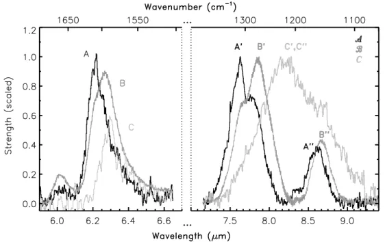
The spectrum presented in Fig. I.2.1 is an example of what AIB features look like in the ISM. However, depending on the astrophysical source, the local physical environment and even redshift the observed AIBs can vary dramatically in profile shape and intensity ratios between different bands. This was well illustrated by Peeters et al. (2002) who classified the different types of observed spectra into empirical classes: A, B and C (see Fig.I.2.4). In terms of interpretation of the origin of the spectral changes, one should consider two aspects: changes in terms of intensity ratios between bands and changes in the shape/position of the band. The most studied intensity ratio is between the
I.2.3 Spectral variations of AIB emission 35 11.3 and 7.7 µm bands. It was clearly shown that this ratio is correlated with flux of the UV field. Thus the lowering of the intensity of the 7.7 µm band regarding to the 11.3µm band was interpreted as due to ionization of PAH molecules (Joblin et al. 1996, 2000; Bakes et al. 2001; Bregman and Temi 2005; Flagey et al. 2006; Galliano et al. 2008b). Interpreting the changes in the shapes/position of the bands has been a subject of debate in the recent years. Though it seems now clear for instance that there is a relation between the strength of the UV field and the position of the 7.7 µm band, the exact physical origin of this shift is unexplained (Bregman and Temi 2005; Sloan et al. 2007).
Figure I.2.4: Variations of the profiles of the 6.2 and 7.7 µm AIBs and their classification (A, B, C) according to Peeters et al. (2002)
I.2.3.2
Inside photodissociation regions
Photodissociation regions (PDRs, Fig. I.2.5) comprise the transition between molecu-lar clouds and the highly irradiated environments of massive stars. In PDRs, the UV photons rule the chemistry and physical processing of dust particles.
Bregman and Temi (2005) suggest that in the NGC 1333-SVS3 PDR the position of the 7.7 µm band is shifted towards 7.9 µm when moving from highly irradiated regions to more sheltered regions. In the Ced 201 reflection nebula, Cesarsky et al. (2000) observed that the width of the 7.7 µm and the continuum to band ratio vary across the nebula. The continuum is weaker and the 7.7 µm narrower in regions where the cloud is more subject to UV irradiation. They interpret this as due to the
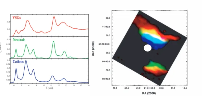
evo-36 Very small dust particles in the cosmic cycle lution of carbonaceous dust: very small grains emitting a continuum and a broad 7.7 µm band are destroyed by UV photons thus releasing free PAHs with no continuum and a narrow 7.7 µm band. In this context, a pioneering work has been achieved by Rapacioli et al. (2005) in order to unveil the origins of the observed spectral variations. They applied single value decomposition (SVD) to spectro-imagery of PDRs obtained with the ISO satellite, to obtain a basis of 3 decorrelated spectra. A set of physically meaningful spectra can then be constructed from linear combinations of the SVD ex-tracted spectra, using a positivity constraint. This constraint is fulfilled by minimizing a criterion that they define and using a Monte-Carlo search. They attribute each ob-tained spectrum (Fig. I.2.6) to populations of very small grains (VSGs), neutral PAHs (PAH0) and positively ionized PAHs (PAH+) respectively. The spatial distribution of
each population can then be reconstructed (Fig. I.2.6).
Figure I.2.5: Schematic view of an photodissociation region seen edge-on. The star situated on the left illuminates the cloud. From Hollenbach and Tielens (1997).
I.2.3.3
Observations of AIB evolution with Spitzer
We have seen in the previous chapter, that the AIBs vary strongly depending on the observed source and sometimes even inside the source. In this context we decided to observe a selection of PDRs using the spectral mapping capabilities of the IRS onboard Spitzer (see description Sect. I.1.4.3). This program (named SPECPDR) is directed by
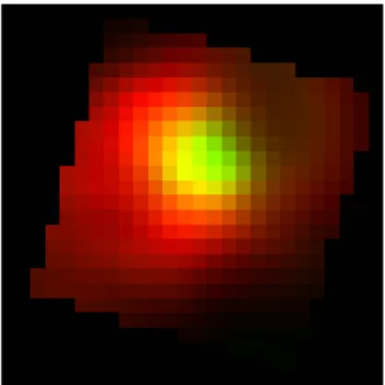
I.2.3 Spectral variations of AIB emission 37 0 0.1 0.2 λ (∝m) 0 0.05 0.1 0.15 0.2 λ (∝m) Iν (A.U.) 6 7 8 9 10 11 12 13 14 15 16 0 0.05 0.1 0.15 0.2 0.25 0.3 λ (µm) VSGs Neutrals Cations 57.6 50.4 43.2 21:01:36.0 28.8 21.6 14.4 30.0 11:00.0 30.0 68:10:00.0 30.0 09:00.0 30.0 08:00.0 RA (2000) Dec (2000)
Figure I.2.6: Left: The three extracted spectra with the SVD + Monte-Carlo method of Rapacioli et al. (2005) and their distribution in the NGC 7023 reflection nebula. The white circle indicates the position of the star which was masked. Note that Red and Green combine to give yellow in the PAH/VSG transition region. Figure adapted from Rapacioli et al. (2005) and Bern´e et al. (2008).
C. Joblin and gathers scientists from CESR and LATT in Toulouse, IAS and LERMA in Paris, and researchers from foreign laboratories such as CSIC in Spain, CalTech and University of Arizona in the USA. In order to sample a wide range of physical conditions to possibly link them to the actual shape of the AIBs we have chosen sources with UV fields of various strengths (see Table I.2.1). The interests of using the IRS are multiple. First it has an unprecedented spatial resolution which enables to better resolve chemical fronts inside PDRs. Second it provides a large field of view which allows to fully map each PDR. Third the spectral resolution is high enough (even in low resolution mode) to fully sample the aromatic bands. Finally, the IRS covers a wavelength range going up to 38 µm enabling to measure the spectrum of very small particles in this unexplored spectral domain (ISOCAM spectro-imagery was only up to 16 µm). We have therefore observed a sample of 11 PDRs (see Table I.2.1) using the IRS in spectral mapping mode and obtained cubes for each one of them (See Sect. II.3.1.1 for description of the data). More recently, and following these observations, another program for Spitzer was accepted (SPECHII, PI: C. Joblin). This program is dedicated to the spatially resolved studies of very small dust particles evolution in very harsh environments. It is also aimed at preparing the Herschel guaranteed time key program WADI (P.I. V. Ossenkopf). We have observed a sample of Hii regions and shock regions presented in Table I.2.2. These observations were achieved using the same strategy as in SPECPDR. Some of these observations are still currently ongoing while some have already been processed. Note that in this thesis I also present results obtained using IRS observations of protoplanetary disks, planetary nebulae and galaxies which have not been obtained as part of the programs presented here but were available on the archive after expiration of the proprietary period.
Table I.2.1: Description of sources in the SPECPDR program
Source Dist. Excitation FUV field Geometry1
(pc) (Teff, spec.type) (Habing)
NGC7023 E 440 17000K, B3Ve 200 E-O
NGC2023 N 450 23000K, B1.5V 1000 E-O, C
Horsehead 450 33000K, O9.5V 100 E-O
IC63 230 30000K, B0.5IV 650 E-O, CG
IC59 230 30000K, B0.5IV 480 E-O
Ced201 420 10500K, B9.5V 200 F-O
Oph filament 160 22000K, B2V 400 E-O, C
Oph SR3 160 13000K, B7 1000 S
L1721 134 22000K, B2IV 10 E-O, CG
California 350 37000K, O7 30 E-O
M31 9e5 UV deficiency
SMC 6e4 low metallicity
1 Geometry codes: E-O: edge-on, C: Cavity, CG: Cometary globule, F-O: Face-on, S: shell
Table I.2.2: Description of sources of the SPECHII program
Region Illuminating Source Distance G0 PDR density
Identification Spectral Type (pc) (Habing) (nH cm−3)
Horsehead Star 09.5V 450 100 ∼ 5 × 10⁴
Rosette Cluster OBV 1600 200 ∼ 1 × 10⁴
Carina-S Star peculiar 2500 400 ∼ 1 × 10⁵
CepB-N Star Association O7/B1 725 1500 ∼ 6 × 10⁴
Mon R2 Cluster B0V 850 5 × 10⁵ ∼ 1 × 10⁶
Objectives of the PhD
Now that the context is set it, is time to consider in which terms we can improve our knowledge on the nature and evolution of carbonaceous dust in our Galaxy (and why not in external galaxies). We have seen in the previous section that AIBs are ubiq-uitous. However their shapes vary strongly depending on the observed astrophysical source. This is likely due to a change of the local physical conditions, which implies a change in the nature of the emitting populations.
Is it possible to understand the observed variations of the AIB emission in a global and self-consistent way, by linking the evolution of very small dust particles populations to the local physical conditions? Can the use of Blind Signal Separation Methods applied to Spitzer spectral cubes help us on this subject?
This manuscript presents an attempt to address the above questions. Its stuc-ture follows somewhat chronologically my progression in the last three years, that was milestoned by the publication of several articles. In Part II we apply so called Blind Signal Separation methods to observations obtained with the Spitzer Space Telescope in order to unveil the pure spectra of different populations of carbonaceous dust. We then compare the spatial distribution of these populations in the NGC 7023 reflection nebulae to the spatial pattern of Extended Red Emission measured with the Hubble Space Telescope. In Part III we propose to use the extracted spectra of the populations identified in Part II in order to reproduce the observed emission of planetary nebulae, protoplanetary disks, HII regions and external galaxies. We show that this is possible only if additional dust populations are added. Thus, using a set of 7 template spectra we show that we are able to reproduce the band emission of all types of sources studied here with limited errors. Finally in Part IV we discuss the implications that these results have on our understanding of the cosmic cycle of interstellar dust and some prospectives.
Part II
Unveiling the spectra of very small
dust particles using Blind Signal
Separation methods
The “pillars of creation” revisited by Laure Cadars. The surface of the pillar-shaped star-forming molecular clouds are irradiated by UV photons of massive stars which
Chapter II.1
Blind signal separation methods
I
n this chapter, we present signal and data processing algorithms knownas Blind Signal Separation (BSS) methods. After a brief introduction, we define the three main families of BSS methods, i.e Independent Com-ponent Analysis (ICA), Non-negative Matrix Factorization (NMF) and Sparse Component Analysis (SCA). For each family we then provide the details of a particular algorithm, to be applied to Spitzer data.II.1.1
Introduction
Blind Signal Separation is commonly used to restore a set of unknown “source” signals from a set of observed signals which are mixtures of these source signals, with unknown mixture parameters (Hyvarinen et al. 2001). It has e.g. been applied in acoustics for unmixing recordings, or in the biomedical field for separating mixed electromagnetic signals produced by the brain (e.g. Sajda et al. 2004). BSS is most often achieved using Independent component analysis (ICA) methods. In particular, the FastICA (Hyvarinen 1999) algorithm was proved to be efficient for recovering source signals. An alternative class of methods for achieving BSS is non negative matrix factorization (NMF), which was introduced in Lee and Seung (1999) and then extended by a few authors. The other main class of methods concerns the algorithms based on sparsity (see definition in Sect. II.1.1.3) of the sources. In the next Sections we provide further details on these three types of methods.
The simplest version of the BSS problem concerns so-called “linear instantaneous” mixtures where the observed signals xi(v) are linear combinations of the unknown
sources sj(v) considered for the same value of the possibly multidimensional variable
46 Blind signal separation methods v on which they depend. For 1D signals depending on a variable λ (as a reference to wavelength for the study of mid-IR spectra) this reads
xi(λ) = r
X
j=1
aijsj(λ) i = 1, . . . , m (II.1.1)
where the ai,j’s are the coefficient of the linear combinations (or weights). This can be
re-written in matrix form as,
X = AS (II.1.2)
where X is an m × n matrix containing n samples of m observed signals, A is an m × r mixing matrix and S is an r × n matrix containing n samples of r source signals. In the context of this work, we have considered only cases in which r ≤ m as in standard investigations. The objective of BSS algorithms is now to recover the source matrix S and/or the mixing matrix A from X.
II.1.1.1
Independent component analysis
The first BSS method was proposed by Herault et al. (1985) and Jutten and Herault (1991), but it was not until 1994 that the concept of Independent Component Analysis (ICA) was generalized (see Comon 1994). BSS methods that rely on ICA are based on the assumption that the sources sj are statistically independent. This means that the
joint probability density of the source sj vector is equal to the product of the marginal
densities: fs(s1, . . . , sr) = r Y j=1 fsj(sj) (II.1.3)
In ICA, the estimation of the source matrix ˆS is obtained by calculating a linear trans-form ˆS = MX that maximizes the independence between the estimated sources ˆsj
which are the rows of ˆS. In pratice, this means optimizing a criterion function F (ˆs) which is a measure of independence. Several criteria have been proposed in the liter-ature, such as maximum likelihood, mutual information, and non-gaussianity. In the following Section, we present one of the most popular ICA method called FastICA, wich is based on the maximization of non-gaussianity.
FastICA
FastICA is a statistical BSS method intended for stationary, non-Gaussian and mu-tually statistically independent random signals (Hyvarinen 1999). It is expressed for zero-mean signals hereafter. In practice, such signals are obtained by first subtracting the sample mean of each observed signal to all signal samples in the corresponding row of X in (Eq. II.1.2). For the sake of simplicity, the notation X refers to these zero-mean signals hereafter. The next step of FastICA consists in applying SVD to the covariance matrix of the observed data, i.e. in deriving a matrix Z of transformed signals defined as
II.1.1 Introduction 47
Z = MX (II.1.4)
where M is selected so that: i) all signals in Z are mutually uncorrelated, ii) each of these signals has unit power and iii) the number of signals in Z is ˆr. The value of ˆr is selected as follows. When applied to the m signals in X, SVD intrinsically yields m output components. Keeping all these components therefore corresponds to selecting ˆ
r = m. Instead, if r < m, one may choose to only keep the ˆr output components which have the highest powers, with ˆr selected so that r ≤ ˆr < m (see details on p. 129 of Hyvarinen et al. 2001 ).This reduces the dimensionality of the processed data and allows one to combine the following two features: i) using ˆr ≥ r still makes it possible to recover all source signals from Z and ii) selecting ˆr < m decreases in Z the influence of noise components which exist in real observations X but were not taken into account in the above data model.
The basic version of FastICA then extracts a first source signal from the matrix Z. The criterion used consists in maximizing the non-Gaussianity of an output signal defined as a linear instantaneous combination of the signals in Z. Therefore, denoting z a column of Z corresponding to a given sample index, the corresponding sample of the output signal reads
y = dTz, (II.1.5)
where the column vector d is constrained to have unit norm. Several versions of the FastICA method have been defined, depending on which parameter is used to measure the non-Gaussianity of y. The most standard parameter is the absolute value of the non-normalized kurtosis, defined for a zero-mean signal y as
Kurt(y) = E[y4] − 3(E[y2])2 (II.1.6)
where E[.] stands for expectation. Various algorithms may then be used for adapting d so as to maximize that absolute kurtosis parameter. Before the FastICA algorithm was introduced, Delfosse and Loubaton (1995) optimized it by using a standard gradient ascent procedure. FastICA is an alternative, fixed-point, optimization algorithm de-scribed in Hyvarinen (1999). It has been shown to yield much faster and more reliable convergence than gradient procedures. Moreover, it does not require one to select any tunable parameter (such as the adaptation gain of gradient algorithms). Once a first source signal has been extracted as an output signal y, FastICA removes its contri-butions from all observed signals contained by X. This yields a matrix X0 which only
contains r − 1 sources. The same procedure as above is then applied to X0 in order
to extract another source. This “deflation” procedure is repeated until all sources are extracted from the observations.
II.1.1.2
Non negative matrix factorization
Unlike ICA, NMF is based on assuming non-negative source signals and mixing co-efficients, without requiring independence of the source signals. It aims to recover the r source signals by approximating the supposedly non-negative matrix X with the following factorization: