BeAMS: a Beacon based Angle Measurement
Sensor for mobile robot positioning
Vincent Pierlot and Marc Van Droogenbroeck Members, IEEE INTELSIG, Laboratory for Signal and Image Exploitation
Montefiore Institute, University of Liège, Belgium
Abstract—Positioning is a fundamental issue in mobile robot applications, and it can be achieved in multiple ways. Among these methods, triangulation based on angle measurements is widely used, robust, accurate, and flexible. This paper presents BeAMS, a new active beacon-based angle measurement system used for mobile robot positioning.
BeAMS introduces several major innovations. One innovation is the use of a unique unsynchronized channel with On-Off Keying modulated infrared signals to measure angles and to identify the beacons. We also introduce a new mechanism to measure angles: our system detects a beacon when it enters and leaves an angular window. We show that the estimator resulting from the center of this angular window provides an unbiased estimate of the beacon angle. A theoretical framework for a thorough performance analysis of BeAMS is provided. We establish the upper bound of the variance and validate this bound through experiments and simulations; the overall error measure of BeAMS is lower than 0.24 deg for an acquisition rate of 10 Hz. In conclusion, BeAMS is a low power, flexible, and robust solution for angle measurement, and a reliable component for robot positioning.
Index Terms—Angle measurement, beacons, infrared detector, mobile robot, robot sensing system, positioning, triangulation.
I. INTRODUCTION
A. Robot positioning
A mobile robot that evolves in its environment cannot navigate or execute its actions correctly without some form of positioning; therefore positioning is a crucial issue in mobile robot applications. Some fundamental papers such as [5], [6], [8], [38] discuss robot positioning. In particular, Betke and Gurvits [5] and Esteves et al. [15] highlight that sensory feedback is essential in order to position the robot in its environment. Some surveys (see [7], [12], [18], [28]) discuss several techniques used for positioning: odometry, in-ertial navigation, magnetic compasses, active beacons, natural landmark navigation, map-based positioning, and vision-based positioning. We can identify two main families encompassing these methods: (1) relative positioning (or dead-reckoning), and (2) global positioning (or reference-based). Techniques belonging to the first family mainly operate by odometry, which consists of counting the number of wheel revolutions (e.g. with optical encoders) and integrating them to compute the offset from a known position; inertial navigation (based on gyroscopes or accelerometers) is less used because of its poor accuracy [7]. Relative positioning based on odometry is very accurate for small offsets, but can lead to an increasing drift resulting from the unbounded accumulation of errors
IR signal
Robot Beacon
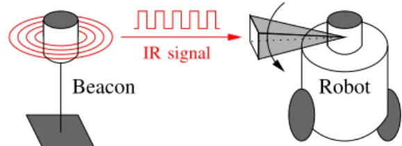
Figure 1: Presentation of BeAMS, a new angle measurement system for mobile robots based on two principles: (1) beacons send On-Off Keying coded infrared signals, and (2) the receiver on the robot turns at constant speed to measure angles of beacons. These angles can be combined to compute the robot position
over time (due to the integration step, uncertainty about the wheelbase, wheel slippage, etc). A global positioning system is thus generally required to recalibrate the position of the robot periodically. On the other hand, global positioning systems are known to be less accurate than odometry, and this is why both methods are essential and complementary to each other [2], [5]. These two informations are generally combined in a Kalman filter or other data fusion algorithm [16], [22]. B. Positioning based on beacons
Most global positioning techniques rely on beacons, whose locations are known, and perform positioning by triangulation or trilateration. In the context of positioning, a beacon is a discernible object in the environment, which may be natural or artificial, passive or active; our system, BeAMS, uses active beacons, and its principle is illustrated in Figure 1. Triangu-lation is the process of determining the location of a point by measuring angles from that point to known locations (beacons) (see Figure 2). This contrasts with the trilateration technique which measures distances from the point to known locations. Because of its robustness, accuracy, and flexibility, triangu-lation with active beacons is widely used for robots [38]. Another advantage of triangulation versus trilateration is that the robot can compute its orientation (heading) in addition to its location [15], [17], [34], which can be as important as the robot position for most applications.
The description of an algorithm that uses angle measure-ments to compute a position or to navigate can be found in many papers, but is not our focus. Triangulation methods using three angle measurements can be found in [10], [14], [15], [17], [27], [34], and methods using more than three angle measurements are described in [5], [38]. More than three angles can be used to increase precision in some pathological
φ1 φ2 φ3 θ B3 x y yR xR R B2 B1
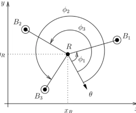
Figure 2: Triangulation setup in the 2D plane. R denotes the robot. Biare the beacons. φiare the angle measurements for Bi, relative to
the robot orientation θ. A triangulation algorithm computes the robot position and orientation based on these angles (three or more).
geometrical setups or to deal with harsh environments where some beacons might be out of sight of the sensor [5], [26], [38], [42]. Note that algorithms dealing with multiple beacons can also work with only three beacons. For our application, we developed a new triangulation algorithm, described in [34]. This paper describes a new angle measurement system, independent of any positioning algorithm. In practice however, angle measurement systems are developed almost exclusively for positioning, as the process of triangulation requires angle measurements. This explains why most authors only evaluate positioning algorithms or present complete systems (hardware and software). As a consequence, it is rare that authors evaluate the performance of the underlying angle measurement system, and there is a lot of confusion about the evaluation criteria (accuracy, precision, resolution, etc). But the quality of positioning depends on the relative configuration of the robot and beacons, and it is essential to evaluate angle measurement separately to improve complete systems. For that reason, we want to evaluate BeAMS directly, and not through a positioning algorithm. In the following, we propose a complete framework to evaluate our system, including two important criteria: the precision (variance), and the accuracy (bias).
The hardware of BeAMS has already been briefly intro-duced in one of our previous paper [31]. A summary of our statistical study on codes and some experiments were presented in another paper [32]. In this paper, we provide an extended description of the hardware and explain all the design parameters and trades-off. We also extend the statistical analysis, discuss the relevance of several comparison criteria, provide a detailed evaluation of the performance of our system, and compare it to other similar systems.
The paper is organized as follows. Section II presents some of the numerous angle measurement systems developed for robot positioning. The hardware of our new angle ment system is described in Section III. The angle measure-ment principles are explained in Section IV. We discuss the parameters and trades-off involved in our system in Section V, and discuss a practical system deployment. A theoretical model, useful for evaluating the performance of our system is detailed in Section VI. Then, in Section VII, we compare
the model to simulation data and real measurements. Finally, Section VIII concludes the paper.
II. RELATED WORK
As explained by Borenstein et al. [7], no universal indoor positioning system exists, contrasting with the widespread use of GPS for outdoor applications. Some surveys on indoor positioning systems may be found in [6], [7], [18], [28]. Technologies used in these systems may be as varied as lasers, IR, Ultrasound, RF including RFID, WLAN, Bluetooth and UWB, magnetism, vision-based, and even audible-sound. In this study, we concentrate mostly on angle measurement systems, although some of the systems include other forms of measurement, such as range. Hereafter, we present a selection of popular commercial systems and then some “home-made” systems found in the literature, all based on beacons. A. Commercial systems
Most commercial systems are described by Borenstein et al. in [6], and also by Zalama et al. in [42] (NAMCO LaserNet, DBIR LaserNav, TRC Beacon Navigation System, SSIM RobotSense, MTI Research CONAC, SPSi Odyssey, LS6 from Guidance Control Systems Ltd., NDC LazerWay, SICK NAV200). Almost all of these systems use an on-board rotating laser beam sweeping the horizontal plane to illuminate retro-reflective beacons. The horizontal sweeping is generally performed with a fixed laser emitter and receiver combined with a 45 deg tilt mirror mounted on a motor. The angular position of the motor is given by an angular encoder attached to the motor shaft. The beacons are generally simple passive retro-reflectors reflecting the light back to the sensor on the mobile robot. Systems using passive retro-reflectors cannot differentiate between beacons, which makes the task of po-sitioning harder. Furthermore a popo-sitioning algorithm working with indistinguishable beacons needs an initial position in order to work properly [21], [42]. In addition, if beacons are not identifiable, the algorithm could fail in the following two cases: at the wake-up (robot start up or reboot) or when the robot is kidnapped (i.e. displaced).
To overcome these issues, some systems use variants such as bar-coded reflective tapes to identify the beacons (for example LaserNav, as used by Loevsky and Shimshoni [26], or robot HILARE [3]). Another technique for identifying beacons consists of using networked active beacons with an additional communication channel (typically an RF channel). When they are hit by the rotating laser, the beacons communicate to compute the angles between them and send the angles back to the mobile through an RF link (MTI Research CONAC). The difficulty with this system is the setup of the networked beacons. The SPSi Odyssey system (used by Beliveau et al. [4]) is different, since it can position a mobile in 3D. The beacons are laser transmitters and the receiver is located on the mobile robot. This system is not able to compute the heading of the mobile (unlike on-board angle measuring systems), except while the system is moving (as in the case of the GPS). Moreover, the field of view of the emitters is limited to 120 deg horizontally and 30 deg vertically, which
makes the positioning possible within a limited volume of space. Nowadays, positioning systems have a full 360 deg coverage, except for the Odyssey and the older LaserNet (90 deg) systems.
It turns out that most commercial systems use rotating lasers combined with retro-reflective beacons. They generally have a good accuracy and working range, but they cannot differentiate between beacons, apart from the LaserNav system, which is no longer manufactured. Finally, they are expensive and take up too much space, which makes them inappropriate for small educational robots. We will now describe home-made systems found in the literature.
B. Non-commercial systems
1) Rotating lasers: One particular famous non-commercial system is the Imperial College Beacon Navigation System [35]. The principle involved in this system appears to be exactly the same as for the CONAC system. This system uses a rotating laser and networked active beacons connected to a base station that sends position back to the mobile via an RF channel. The main drawback of these systems is the wiring and setup of the beacons. To overcome this issue, a more recent system, similar to the Imperial College Beacon Navigation System and CONAC, is presented by Zalama et al. [42]. It uses an on-board rotating laser and active beacons that send their identifier back to the mobile with some RF coded pulses when they are hit by the rotating laser. The beacons are totally independent and stand-alone (no network, communication cables or base station), which makes the setup easier.
Even if these systems solve the beacon identification prob-lem, there is an open issue: how do such systems behave when multiple robots use the same setup of beacons? A beacon would send its identifier back to all robots even if only one of them has hit that beacon, causing false angle measurements to the other robots. So we guess that these systems are inadequate for being used by multiple robots simultaneously.
2) Static receivers: In general, the 360 deg horizontal field of view is covered by a single receiver combined with a rotating system. However, it is possible to cover the whole horizontal plane without mechanical part, as explained here-after. The first type of static sensor system uses multiple static receivers uniformly distributed on the perimeter of a circle. These systems measure the angles to the beacons by simply “looking” at which receiver receives the signal from a beacon. Since more than one receiver can receive the same signal, an interpolation can be performed to improve the angular position of a beacon, as highlighted by Gutierrez et al. [19] and Roberts et al. [37]. These systems generally also derive a distance to the beacons. For example, some of these systems [19], [23], [36], [37] use the infrared received signal strength to compute the distance to the beacon, in addition to the bearing information. In [20], Hernandez et al. compute the distance using the aperture angle of the received signal (time taken to sweep the receiver). In [13], Durst et al. use Nintendo Wii cameras instead of infrared receivers to localize and identify the different beacons. Lee et al. [25], and Arai and Sekiai [1] use infrared light from beacons and measure the incident
angle of the infrared light with two fixed photodiodes and a specialized circuit. Another similar idea consists in the use of only one static receiver or laser emitter. The 360 deg field of view is obtained by the rotation of the robot itself, which is expected to move to see the beacons [29], [40]. The main drawback is that the position update rate depends on the robot movements and is generally low compared to other systems.
These systems have the benefit of being small, lightweight, and simple (no moving part). Unfortunately, it turns out that these systems are less accurate (5 → 10 deg) than rotating sensors (0.05 → 0.5 deg), and that the accuracy of the angles depends on the number of sensors. They are often used by swarm of robots for relative positioning and communication, but not for precise global positioning.
3) Panoramic cameras for detecting beacons: The second type of static sensor systems uses panoramic cameras to measure angles or distances. A common way to measure angles with a static camera and without moving parts is to transform it into an omni-directional camera via a catadioptric mirror, fish-eye lens, or a reflecting ball, as proposed by Betke and Gurvits [5]. With this configuration, a 360 deg horizontal field of view of the scene is taken in one image. The angular positions of the beacons are computed through image processing by searching the beacon patterns whithin a circular region of the image. Jang et al. [22] base their system on the same principle with only one beacon, but they also compute the distance to that beacon.
One distinctive feature of panoramic cameras is that angles to beacons are measured at the same time, in one image. This can be an advantage if the positioning algorithm uses a triangulation technique directly. This advantage is useless if the angles are fed into an Extended Kalman Filter, which can take advantage of one angle at a time. Panoramic cameras also need a more complicated image processing algorithm, and they depend highly on lightning conditions. Finally, like the multiple static receivers, they are less accurate than rotating systems.
4) Most closely related systems: One of the oldest systems, related to ours, is described by McGillem and Rappaport in [27]. That system is made up of beacons emitting infrared modulated signals and a rotating infrared detector mounted on a turntable to measure the angles to the beacons. Another recent and similar system is proposed by Brkic et al. in [9]. This system relies on infrared beacons and a rotating receiver; a brushless DC motor with rotary transformer overcomes the problem of contact-less power supply, and ensures signal transfer. Unfortunately, no information about motor control, infrared codes, or angle calculation is provided in that paper. Finally, the accuracy of the system is given in terms of distance errors on the moving area, and no information about the accuracy of measured angles is given. Kemppainen et al. [24] also describe a system similar to ours for multi-robot spatial coordination, the system being used for inter-robot relative positioning, not global positioning. The difference with the previous systems is that the infrared emitting beacons are located onto the robots themselves, instead of being at fixed locations. In addition to the angle measurement, the system estimates the range by the received signal strength. Using
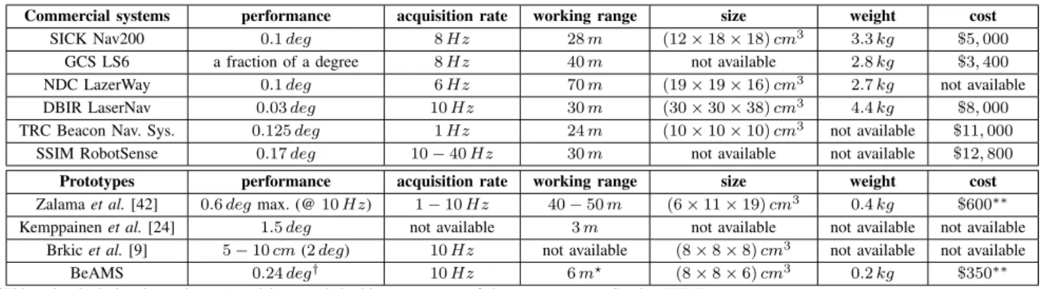
Commercial systems performance acquisition rate working range size weight cost
SICK Nav200 0.1 deg 8 Hz 28 m (12× 18 × 18) cm3 3.3 kg $5, 000
GCS LS6 a fraction of a degree 8 Hz 40 m not available 2.8 kg $3, 400
NDC LazerWay 0.1 deg 6 Hz 70 m (19× 19 × 16) cm3 2.7 kg not available
DBIR LaserNav 0.03 deg 10 Hz 30 m (30× 30 × 38) cm3 4.4 kg $8, 000
TRC Beacon Nav. Sys. 0.125 deg 1 Hz 24 m (10× 10 × 10) cm3 not available $11, 000
SSIM RobotSense 0.17 deg 10− 40 Hz 30 m not available not available $12, 800
Prototypes performance acquisition rate working range size weight cost
Zalama et al. [42] 0.6 degmax. (@ 10 Hz) 1− 10 Hz 40− 50 m (6× 11 × 19) cm3 0.4 kg $600∗∗ Kemppainen et al. [24] 1.5 deg not available 3 m not available not available not available
Brkic et al. [9] 5− 10 cm (2 deg) 10 Hz not available (8× 8 × 8) cm3 not available not available
BeAMS 0.24 deg† 10 Hz 6 m? (8× 8 × 6) cm3 0.2 kg $350∗∗
†This value includes the variance (precision), and the bias (accuracy) of the measures (see Section VII-F).
?The prototype is optimized for that range value, typical for the EUROBOTcontest. In Section V-B, we explain how to increase the working range up to 36 m. ∗∗The cost is calculated for the hardware components only (one sensor and three beacons).
Table I: Comparison of different angle measurement systems.
the bearing and the range, a robot can compute the relative position of all other robots.
These systems (emitting beacons, and rotating receiver) are able to identify the beacons while using only one communi-cation channel (the beacon signal itself). Due to the nature of this unidirectional channel, multiple receivers (robots) can receive the signals from the same beacons at the same time without disturbing each other (like for the GPS system). But, unlike reflective tape, beacons have to be powered up. C. Summary
There is a large variety of angle measurement systems. Some systems do not identify the beacons, and others require more than one communication channel. Some systems cannot position multiple robot simultaneously. If we compare the values found in the literature, it turns out that rotating sensors are more accurate than fixed sensors, but have the disadvantage that information and power have to be transmitted to the sensors, if these are located on the turning part of the system. A fixed sensor can be used, if combined with a mirror and a motor to sweep the horizontal plane and cover a 360 deg field of view. With a mirror, the light rays are redirected to cross the rotation center of the turning system. In general, the mirror is mounted on a hollow gear, which is driven by the motor through a gear or belt, allowing light rays to pass and reach the sensor. This solution tends to make the mechanical part of rotating systems more complicated and cumbersome. It turns out that the most flexible solutions are rotating lasers with passive bar-coded reflective tapes or active emitting beacons with a rotating receiver. This last solution requires to power-up the beacons. A comparative table of some commercial and home-made systems and their characteristics is provided in Table I. For some systems, implementation characteristics are missing or incomplete, such as the working distance, power consumption, dimensions, etc. Finally, evaluation criteria such as precision (variance), accuracy (bias) and resolution (number of steps for one turn) are sometimes confused during the per-formance analysis. Also, some systems are evaluated through a positioning algorithm, and therefore it is a hard task to evaluate the quality of the underlying angle measurements to compare systems.
The comparative table shows that BeAMS is small and lightweight. In addition, BeAMS proposes a new mechanism for angle measurement and uses an unsynchronized channel with coded signals to identify beacons.
III. HARDWARE DESCRIPTION OF A NEW SYSTEM
While there are many angle measurement systems, none of them was suited for our application, as explained hereafter. Our first motivation for this work was to create a new system for the EUROBOT contest1, which imposes many constraints. For the positioning part, the most important constraints are: (1) the available volume for the hardware on the robot is limited to (8 × 8 × 8) cm3, (2) home-made laser systems are prohibited except if they are manufactured and kept in their house cases. The EUROBOTcontest is a harsh environment for robot position. Firstly, as collisions and shocks are numerous, the knowledge of beacons IDs is an advantage to be robust to the wake-up or kidnapped issues. Secondly, the environment is polluted by many sources of noise including infrared, lasers, radio waves, and ultrasound signals. Also the lightning conditions are very bad and there are lots of shiny or reflective surfaces. Finally, more than one robot per team may evolve on the field.
Considering all these constraints, the system has to identify the beacons, use coded signals, and allow multiple robots. Commercial system were unsuitable because of their sizes, their high price, and because they cannot identify the beacons. Home-made laser systems are prohibited. Static receivers do not provide the accuracy needed for this contest. Finally we wanted to use a triangulation based positioning to estimate the robot heading precisely (this is important since the heading is highly downgraded by odometry). So we designed an angle measurement system based on beacons emitting infrared coded signal and a rotating receiver. Note that, to our knowledge, there is only one very similar system, designed by Brkic et al. [9], also for the EUROBOT contest. But, according to the
authors, their system is not accurate enough to position the robot (see Table I).
φ1 φ2 φ3 R B1 B3 B2 θ
Figure 3: Schematic top view representation of the system. The system is composed of: (1) several active beacons Bi emitting
infrared light in the horizontal plane, and (2) a sensor located on the robot R. The aim of the sensor is to measure the azimuthal angles φiof the beacons in the robot reference determined by θ.
BeAMS is original but it has the same limitations as any other optical system, as explained in [7], [28], [42]. First, a line of sight between beacons and sensor has to be maintained for the system to work. Also, the reflections of beacon signals on shiny surfaces can lead to false detections. Finally, the sensor could be blinded by direct sunlight (causing the SNR to decrease). This has the effect of reducing the working range in outdoor conditions.
A. Architecture of BeAMS
The hardware of BeAMS consists of a sensor located on the robot, and several active beacons emitting infrared light, located at know positions. This configuration is represented in Figure 3. As illustrated in this figure, the aim of the sensor and processing unit is to determine the identifier of each beacon i, as well as its azimuthal angle φi, in the robot reference, whose orientation is given by θ. The sensor is composed of an infrared receiver/demodulator and a motor. The beacons are infrared LEDs whose signal is modulated. To achieve the angle measurements, the infrared receiver is combined with the motor turning at a constant speed. One of the key elements of our system is that the receiver sweeps the horizontal plane at constant speed, and that the relationship between the angle and time is very precise. In order to identify beacons and to increase robustness against noise, each beacon sends out a unique On-Off Keying (OOK) amplitude modulated signal over a 455 kHz carrier frequency. Furthermore, BeAMS only requires one infrared communication channel; there is no synchronization channel between the beacons and the robot, which allows multiple robots to share the same system. Finally, the mechanical part of the system is kept as simple as possible (motor only), with no gear system or belt, thanks to the hollow shaft, and no optical encoder for the motor control or angle measurement is needed. These features make BeAMS a small, low power, flexible, and tractable solution for robot positioning. BeAMS has been continually improved since its inception and has been used successfully in the EUROBOT
contest for the last four years. In the next sections, we describe the hardware components of our system.
µC
ModulatedCarrierPower
Stage
IR LED
ID
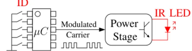
Figure 4: Architecture of a beacon. The central element of a beacon is an infrared LED. A PIC microcontroller (µC) generates the appropriate signal to drive the IR LEDs through the power stage. Each beacon emits its own unique IR signal continuously so that the receiver can determine the beacon identifier (ID).
Figure 5: Picture of a beacon. The main part of a beacon is made by IR LEDs, which are located under the printed circuit board, parallel to the moving area and directed towards the center of the moving area.
B. Description of the beacons
The core of a beacon is composed of IR LEDs (SFH485P); they emit signals in a plane parallel to the moving area. These LEDs have a large emission beam so that a small number of LEDs per beacon can cover the whole area. A PIC microcontroller generates the appropriate signal to drive the IR LEDs through the power stage. Each beacon continuously emits its own unique IR signal so that the receiver can determine the beacon’s identifier (ID). Figure 4 represents the schematic architecture of a beacon and Figure 5 shows a picture of a beacon. The power consumption is 100 mA at 9 V, for a working distance of up to 6 m.
C. Description of the sensor
As shown in Figure 6, the sensor is composed of a mini stepper motor, a 12 mm convergent lens, a small front surface mirror with a 45 deg tilt, a polycarbonate light guide placed in the center of the motor shaft (which has been drilled for this purpose), an IR receiver (a TSOP7000 from VISHAY) and an
optical switch used to calibrate the zero angle reference θ (see Section IV-B). The lens and mirror are placed on a “turret”, which is fixed to the motor shaft. The receiver is fixed to the bottom of the motor, just under the light guide. This con-figuration allows IR signals from a beacon to reach the fixed receiver through the entirely passive “rotating turret” and light guide. As a result, the receiver can virtually turn at the same speed as the turret. By introducing this original disposition of optical elements into our system, the system behaves as if the receiver is turning without the mechanical constraints and inconvenience. Finally, a PIC microcontroller is used to drive the motor through its controller and to decode the output
µC
OS
R
LG
T
SM
S
C
M
B
iL
Figure 6: Schematic representation of the receiver. Bi is a beacon
emitting IR light, L is the lens, M is the mirror, LG is the light guide, Ris the receiver, SM is the stepper motor, S is the hollow shaft, T is the turret, C is the motor controller, µC is the PIC microcontroller, and OS is the optical switch.
Figure 7: Picture of the sensor with the rotating turret in black (top) and the lens, the stepper motor (middle), the optical switch (middle right), and the electronic card (bottom).
of the receiver. Figure 7 shows a picture of the sensor. The entire sensor weights 195 g, and the power consumption is 47 mA at 9 V . Now that the hardware elements have been presented, we detail some elements of the system: software architecture, motor control, angle measurement principle, and infrared codes.
IV. MEASUREMENT PRINCIPLES OFBEAMS
A. Software description
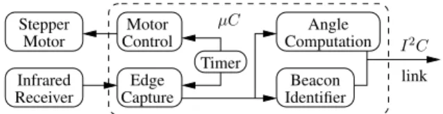
The software building blocks of BeAMS are drawn in Figure 8. The key principle of the software is to use a common timer to drive the stepper motor at a constant speed, and to capture the receiver output edges. The receiver output is connected to a capture module in the microcontroller. On a falling or a rising edge of the receiver output, this module latches (captures) the actual timer value to a register that may be read later by the software. This allows us to associate a time to each incoming event (falling or rising edge). And as the value of the timer is perfectly linked to the motor angular position, the association of an incoming receiver event to an angular position is as accurate as possible. The captured values serve to compute the angular position of the beacons and their IDs.
B. Stepper motor control
The stepper motor is driven in an open loop via an input square signal to advance the motor step by step. The stepper
µC Stepper Motor Infrared Receiver Motor Control Edge
Capture IdentifierBeacon
ComputationAngle I2C link Timer
Figure 8: Software organization of BeAMS. µC is the PIC micro-controller. A common timer is used to drive the stepper motor at a constant speed and to capture the edges of the receiver output. These captured values are used to compute the angular positions of the beacons as well as the beacon identifiers.
motor has 200 real steps and is driven in a half-step mode via its controller, which turns the number of steps into 400. The frequency of the step signal controls the rotation speed of the motor and is derived from the common timer. Since the timer is 156 times faster than the step signal, we achieve a sub-step time resolution so that the number of “virtual” steps is 400 × 156 = 62400 exactly. The motor turns at a constant speed ω and the angular position of the turret/receiver φis thus proportional to the value of this timer. Whereas the motor is controlled step by step, the rotation is assumed to be continuous due to the high inertia of the turret compared to the motor dynamics. Since the motor turns at a constant speed, the common timer value can be seen as a linear interpolation of the motor position between two real steps of the motor.
This kind of control in open loop with a stepper motor is possible since the torque is constant and only depends on the turret inertia and motor dynamics, which are known in advance. The advantage of this approach is that we do not need a complicated control loop or expensive rotary encoder in order to detect the position of the turret with precision. Indeed, the common timer acts as a rotary encoder, and the position of the turret can be obtained by reading the value of the timer. As explained earlier, there are 62400 “virtual” steps of the motor. The angular resolution is thus given by 360/62400 = 0.00577 deg (0.1 mrad). The timer clock runs at 625000 Hz, to give an angular speed of625000/62400= 10.016turn/s. Since the motor can start from or stop at any angular position, an optical switch (denoted OS in Figure 6) is used to calibrate the zero angle reference θ by reading the timer value when the turret passes through the switch.
C. Angle measurement mechanism
Let us denote by φ the current angular position of the turret/receiver, relatively to θ. As the turret turns at a constant speed ω, the angular position φ is directly proportional to time
φ(t) = ω t. (1)
As a result, we can talk about either time or angular position indifferently. For convenience, we prefer to refer to angles instead of time units.
The TSOP7000 is a miniaturized IR receiver that acts as an OOK demodulator of a 455 kHz carrier frequency. The input is a modulated signal whose carrier wave is multiplied by the “0” or “1” binary message. The receiver outputs a value “1” when it detects the carrier wave and “0” otherwise. No other information is given by the receiver. By design, the
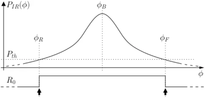
Pth φ φB PIR(φ) R0 φF φR
Figure 9: The upper curve PIR(φ) is the expected infrared power
collected at the receiver while the turret is turning. R0 represents
the receiver output for a non modulated infrared carrier wave (pure 455 kHzsine wave). The black arrows represent the measured values respectively for φR to the left (first Rising edge) and for φF to the
right (last Falling edge).
receiver combined with the optical components has a narrow field of view and, consequently, the amount of infrared power collected at the receiver, denoted by PIR(φ), depends on the angle. This power also depends on the power emitted by the beacon, and the distance between the beacon and the receiver. Note also that the exact shape of PIR(φ) depends on the hardware, that is the receiver, optical components, and the geometry of the turret. It is impossible to derive the precise power curve from the specifications, because we only have access to the demodulated signal, and no information about power is available. Therefore, we make some basic assumptions regarding the shape of PIR(φ); the resulting expected curve PIR(φ)is shown in Figure 9. The exact shape of this curve does not have much importance in this study but is assumed to increase from a minimum to a maximum and then to decrease from this maximum to the minimum. In the following theoretical developments, we make three important assumptions about the curve and the detection process itself: 1) The maximum coincides with an angle, which is the
angular position of the beacon, denoted φB (i.e. the angle we want to measure). As a result, for any angle φ PIR(φ)≤ PIR(φB). (2) 2) The curve is supposed to be symmetric around the maximum since the turret and all optical components are symmetric. This means that
PIR(φB− φ) = PIR(φB+ φ). (3) 3) Finally, we assume that the receiver reacts to 0 → 1 and 1→ 0 transitions at the same infrared power threshold Pth, respectively at angles φR and φF
PIR(φR) = PIR(φF) = Pth. (4) This hypothesis will be discussed later, in Section VII-F. From equations (3) and (4), we derive that φB−φR= φF−φB and that
φB=
φR+ φF
2 . (5)
This equation expresses an important innovation that has two benefits: (1) we derive the angle of the beacon not from the maximum power, but from two angle measurements that
take the narrow receiver optical field of view into account, and (2) by measuring an angular window (that is two angles) instead of one angle, it is possible to analyze the temporal evolution of the signal inside this window to determine the code of the beacon (or any other kind of useful information). Note that the angular window, defined as φF − φR, depends on the received IR power. It increases if the received power increases, and decreases if the received power decreases.
First, we assume that the beacons send a non modulated IR signal, that is a pure 455 kHz sine wave and explain the measurement principle for one beacon; the principle is the same for any number of beacons. While the turret is turning, the receiver begins to “see” the IR signal from that beacon when the power threshold Pth is crossed upwards (0 → 1 transition). The receiver continues to receive that signal until Pth is crossed downwards (1 → 0 transition). The receiver output is depicted as R0 in Figure 9. At these transitions, the capture module latches values for φR and φF. The angular position of the beacon is then computed after equation (5). D. Beacon identifier and infrared codes
The convenient assumption of continuous IR signals used in the previous section is not realistic because (1) we would not be able to distinguish between the different beacons, and (2) it is essential to establish the beacon ID (especially in a very noisy environment like the EUROBOT contest where other IR
sources may exist).
In BeAMS, each beacon emits its own code over the 455 kHz carrier wave; this emission is continuous so as to avoid having any form of synchronization between the beacons and the receiver. As a result, each beacon signal is a periodic signal whose period corresponds to a particular code defining the beacon ID. The design of these codes is subject to several constraints related to (1) the receiver characteristics, (2) the loop emission, (3) the desired precision, (4) the system’s immunity against noise, and (5) the number of beacons. We elaborate on these constraints below:
1. Receiver. The TSOP7000 requires that the burst length (presence of carrier wave) be chosen between 22 and 500 µs, the maximum sensitivity being reached with 14 carrier wave periods (14/455000 = 30.8 µs). The gap time between two bursts (lack of carrier wave) should be at least 26 µs. 2. Loop emission. Because of our willingness to avoid a synchronization between beacons and the receiver, we must ensure that the periodic emission of a code does not introduce ambiguities. For example [0101] is equivalent to [1010] when sent in a loop. Thus any rotation of any code on itself must be different from another code.
3. Precision. The lack of synchronization between beacons and the receiver introduces a certain amount of imprecision. Indeed, the first received IR pulse may be preceded by a gap time corresponding to a zero symbol. This affects the estimation of φR. The same phenomenon occurs for φF. A fairly obvious and intuitive design rule would say that we have to reduce the duration of zeros, as well as their frequency of appearance. Therefore, we forbid two or more consecutive zeros, and the duration of one zero (the gap time) must be
1 1 1 1 0 1 1 1 1 1 1 0 1 1 1 1 1 1 1 1 1 0 1 1 1 1 1 1 1 1 1 0 1 1 1 1 1 1 1 1 1 0 1 1 1 1 1 1 1 1 1 0 0 0 0 0 1 1 1 1 t C1 t t C3 t C4 t C5 C2 Tc= 12Tb (Tb= 30.8 µs)
Figure 10: Temporal representation of the C1, C2, C3, C4 and
C5 codes. These codes are repeated continuously and multiply the
455 kHzcarrier wave to compose the complete IR signal.
reduced as much as possible (see Section VI) for further explanations about the error due to the gap time).
4. Immunity. The codes should contain enough redundancy to be robust against noise or irrelevant IR signals.
5. Number of beacons. The codes should be long enough to handle a few beacons, but as short as possible to be seen many times in the angular window associated to a beacon, thus improving the robustness of the decoding.
All these constraints lead us to propose this family of codes: Ci= [1i0112Nc−i01] i = 1, . . . , Nc (6) where Nc denotes the number of codes in the system. The duration of a bit is set to Tb = 30.8 µs since this value maximizes the receiver sensitivity, while respecting the min-imum gap time. Although not mandatory, the duration of a one symbol has been chosen to be equal to the duration of a zero. This is to simplify the implementation of the beacons and to ease the decoding process. The gap time is the same for all codes and corresponds to the duration of a unique zero symbol. The second half part of the codes can be seen as a checksum, since it makes the number of ones constant (2Nc). In our current implementation, we have Nc= 5codes because this is appropriate for our application. Figure 10 shows the temporal representation of the codes for Nc = 5. Note that any code meeting the second requirement (differentiable under loop emission) would work to identify the beacons. However, they may not meet the third requirement if the zero symbols appear in random patterns. Indeed, a thorough analysis about the error introduced by the gap time (see Section VI) shows that this error increases with the frequency of zero symbols and with the square of the zero duration. Moreover, a simulator (see Section VII-C) has been created to validate this result. This simulator helped us to compare codes w.r.t. the error they generate. From our experience, the codes presented in expression (6) are the best ones that meet all our requirements, but we have no formal proof of it.
The angle measurement principle still operates exactly as in Section IV-C even if the IR carrier wave is modulated by the codes. Since there are gap times in the IR signal of a beacon, there are more than two edges in the received signal. The intermediate edges are used to determine the beacon ID, by analyzing the durations of burst lengths and gap times. But the first and last edges of the received signal always correspond to our measurements of φR and φF. These two edges are isolated from all other edges due to a timeout strategy, which
C3 C5 C3+ C5 -1 0 1 2 3 4 5 6 0 0.0005 0.001 0.0015 0.002 0.0025 0.003 0.0035 Recei ver Output (V ) Time ( s)
Figure 11: Image of an oscilloscope screen displaying the receiver output voltage. In this experimental setup, two beacons emit the codes 3 and 5, respectively. The beacons and the receiver are placed so that the signals slightly overlap. Despite that, it is possible to distinguish both codes in the signal.
relies on the fact that the separation time (or angle) between two different beacons is much greater than the separation time between consecutive edges in a code. Actually, the separation time is set to four bit durations, which corresponds to a separation angle equal to 0.44 deg.
Note that, for the proper functioning of the system, it is important that the receiver collects infrared light from one beacon at a time. To do this, some additional optical components are used to limit the field of view of the receiver to a narrow value (a few degrees). However, despite the narrow field of view, and the timeout strategy to separate beacons, two or more beacons might appear in the same angular window if they are close enough (from an angular point of view). When this situation occurs, the demodulated signal is composed of codes from the different beacons, and they appear in the same order as the turret turns and sees the different beacons. This means that the timeout strategy is not able to cut the different signals. Also, at the transition points, the signal could be composed of burst or gap durations that do not correspond to any code. The decoding algorithm simply adds (in counters) the number of different codes it sees, as well as bad durations. Therefore, the receiver is capable to differentiate between a pure signal from one beacon, or a compound signal from several beacons. The system can then decide to keep or reject a compound signal; this capability to check the consistency of codes is an important advantage of BeAMS. To illustrate this capability, we provide the image displayed by an oscilloscope showing the receiver output voltage for two beacons emitting the codes 3 and 5, respectively (see Figure 11). In this figure, the receiver can easily detect that two beacon signals overlap slightly.
V. PRACTICAL CONSIDERATIONS
A. Parameters and trades-off
The design of BeAMS implies many parameters and some trades-off that need to be explained. First of all, we had to
choose a turning speed (or acquisition rate). Lots of com-mercial or non comcom-mercial systems works at 10 Hz, which seems sufficient for a robot moving at moderate speed. Also, the accuracy of these systems is more likely to be 0.1 deg, to get a reasonable accuracy on the final position. Our system uses an OOK modulation that leads to an error due to the gap times (T0). Our statistical analysis, as well as our simulator confirm this result. However, it is easy to show that the maximum absolute angular error is given by φ0= ω T0, since the turret has turned by this angle during a gap time. This equation represents the most important trade-off: for a given receiver, increasing the rotation speed would increase the error on measured angles. We decided to choose the smallest T0, and afterwards the maximum turning speed according to the maximum error accepted. In our case, the TSOP7000 was the only receiver providing the minimum gap time satisfying the pair of parameters φ0and ω. Then the optical field of view has been tuned with optical components to be narrower, but large enough to receive some bits/codes from one beacon in the angular window, for this turning speed. Typically, we receive a minimum of 20 bits (∼ 2 codes) at the maximum range, which corresponds to the smallest angular window. So, for a given receiver, this maximum working distance depends on the emitted power combined with the size of the lens, and the minimum number of bits we need to identify the beacons. These parameters have been chosen to meet the EUROBOT
rules. The lens/focal distance has been chosen to hold in the allowed volume. Then the emitted power has been tuned to reach the maximum distance possible on the moving area. Indeed the system works until 6 m, which is greater than required.
B. System deployment
BeAMS was designed for the EUROBOT contest. However,
the system could be used in any other application involving angle measurements based positioning. Two parameters are important to use BeAMS in another context: (1) the working distance, and (2) the number of beacons.
Obviously, the covered area is determined by the maximum working distance. The current version of BeAMS reaches 6 m with a small lens (12 mm) and usual LEDs. This distance can be increased either by increasing the size of the lens, or by rising the emitted power. In our application, the size of the lens is limited since the available volume is limited. The emitted power can be increased either by choosing other IR LEDs or by increasing the number of LEDs. For example, multiplying the emitted power Pe by four, and the surface of the lens S by nine would multiply the working distance d by six, as d is proportional to√SPe. With our prototype, we would reach a distance of 36 m, which is comparable to commercial systems. Then we have to consider the number of beacons. Although Figures 2 and 3 represent the system with three beacons, it is important to note that the sensor can measure angles for any number of beacons, three being the minimum number to achieve correct positioning. We chose a code family that allows 5 beacons because it was sufficient for our application. With the same code family, we can go up to 9 beacons since
we are limited by the maximum burst length permitted by the receiver. However, we can use any other codes respecting the constraints of the receiver, as explained in Section IV-D. The number of codes is limited by the minimum number of bits we receive at the maximum working distance. This minimum number of bits received in the time window is fixed by the optical field of view combined with the rotation speed, as expressed by equation (1). As explained previously, there is a trade-off. Increasing the rotation speed decreases the time window, and subsequently the number of bits and the number of possible codes. In our application, the minimum number of bits is more or less 20, at the maximum range with a turning speed of 10turn/s. As explained in Section IV-D, we use a checksum and we want to see the code many times in the time window. From a practical point of view, 10 of these 20 bits could be used to code the beacons, without jeopardizing the noise robustness. This allows for a maximum of 1024 beacons. But then we have to consider the beacon spacing and multiple beacon detection issue. As explained in Section IV-D, the signals from different beacons could appear in the same time window if they are too close (from an angular point of view). This has the effect of corrupting the angle measurements of those beacons. Fortunately, the system is able to detect these pathological cases and it then rejects measurements due to code collisions, unlike laser systems with retro-reflective stripes. In a practical application, code collisions occur when the beacons are almost aligned (a few degrees of angular separation). However, beacons are placed against walls or in corners, where it is unlikely to find the robot. Some papers discuss the issue of beacon placement. Algorithms to find the best place of a minimum number of beacons to meet a given criterion, most often a minimum positioning error, are proposed in [11], [39], [41]. For BeAMS, there is only one additional constraint: anywhere on the moving area, the receiver has to find at least 3 beacons, not aligned with any other beacon. Finally, note that the decision to choice a passive sensor and active beacons was guided by the EUROBOTcontest. It is possible to swap some design choices, for example which elements are passive or active, for other specific industrial setups.
VI. CODE STATISTICS AND ERROR ANALYSIS
Now that the system has been presented, we concentrate on the errors that affect angle measurements. One can identify two kinds of noise in BeAMS: (1) the natural noise, and (2) the artificial noise. Like for all other systems, BeAMS is affected by the natural noise, due to the receiver output jitter, rotation jitter, electronic noise, other infrared signals, etc. In addition to the natural noise, BeAMS is affected by another kind of noise due to the codes and the use of an OOK modulation. In order to identify the different beacons, we decided that each beacon has to send its own coded signal. Unfortunately, this strategy produces errors when no signal is sent, that is during an OFF period of the sequence, as explained in Section IV-D. In the following explanation, this is interpreted as an additional noise due to the OOK modulation mechanism. But, unlike the natural noise, the artificial noise can be controlled, and it is
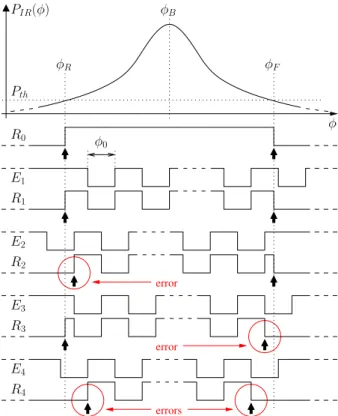
Pth φ φB PIR(φ) R0 R1 R2 R3 E1 E2 E4 R4 φF φR φ0 errors error error E3
Figure 12: The upper curve PIR(φ)is the infrared power collected
at the receiver while the turret is turning. Eiare examples of emitted
signals from the beacons. Riare the corresponding received signals
at the receiver output. R0 is the special case corresponding to the
non modulated infrared carrier wave (no OFF periods). The black arrows represent the measured values respectively for Φr to the left
(first Rising edge) and for Φf to the right (last Falling edge). The
encircled arrows emphasize errors made on Φr or Φf.
important to evaluate the level of artificial error to guarantee the usability of BeAMS in real conditions. Therefore, we first focus on the artificial noise to evaluate the error made on measured angles resulting from the coding of beacon signals. The natural noise is discussed in the next section. Because of the OFF periods in the codes, there are no means to access the true values of φRand φF. Therefore, we consider random variables instead, denoted by Φr and Φf. According to (5), we propose the following estimator Φb for the true beacon angular position φB:
Φb=
Φr+ Φf
2 . (7)
A. Description of the errors
As the receiver captures an OOK amplitude modulated signal, it can only detect the presence of the carrier wave (denoted by a 1 or ON period) or the absence of the carrier wave (denoted by a 0 or OFF period). Let us now examine the influence of the OFF periods on the first rising and last falling edges. As illustrated in Figure 12, if a beacon emits a 1when it enters into the angular window, there is no error on Φr. However, if a beacon emits a 0 when it enters the angular window, there is an error on Φr because the receiver misses the actual 0 → 1 transition. In fact the transition occurs later
(Φr ≥ φR), at the next 1. The same consideration applies to Φf, except that the 1 → 0 transition could occur sooner (Φf ≤ φF). All these specific situations are illustrated in Figure 12. We first represent the output of the receiver for a non modulated carrier wave, R0. In that case, there are no errors in the transition times because the beacon sends out a continuous 1 symbol. The four other cases represent the output of the receiver for four different situations using an arbitrary code (we use here a simpler code than ours for the purpose of illustration, but this does not change the conclusions). The first case, corresponding to the received signal R1, does not induce any error because Pth is crossed upwards and downwards when the beacon emits a 1 symbol. The second case (R2) generates an error on Φr only. The third case (R3) generates an error on Φf only, and the fourth case (R4) generates an error on both Φr and Φf. From Figure 12, one can see that the receiver output Riis the logical AND between Eiand R0. Of course, this an ideal behavior of a practical receiver, and this hypothesis will be discussed later.
Assume now that the OFF periods of a sequence all have the same duration, denoted by T0 (this is our choice by design). Because the motor rotates at a constant speed, an OFF period is then equivalent to an OFF angle called φ0. The worst case for estimating Φroccurs when an OFF period starts at an angle φ = φR, delaying the next transition to an angle φR+ φ0. The same reasoning applies to Φfwhen an OFF period begins at an angle φ = φF−φ0. In both cases, the maximum absolute error on Φror Φfis equal to φ0. These are the worst cases but there are many combinations of these two errors. In the following sections, we establish the probability density functions (PDFs) of the random variables Φr and Φf, and derive characteristics of the estimator Φb.
B. Notations
• N0, N1 are the number of 0’s or 1’s in a code, respec-tively.
• p0, p1 are the probabilities of obtaining a 0 or a 1 respectively at the IR power threshold (rising or falling edge), that is their frequencies. By definition we have p0=N0/N0+N1, p1=N1/N0+N1, and p0+ p1= 1. • T0 is the OFF period (duration of a 0) in a code. The
only assumption is that the OFF periods of a code must all have the same duration.
• φ0 is the OFF angle. It corresponds to the angular displacement of the turret during the OFF period T0:
φ0= ω T0. (8)
In our application, we have: N1= 10, N0= 2, p0=1/6, ω = 10.016turn/s, T0 = 30.8 µs, and φ0 = 0.111 deg, for each code.
• The Uniform PDF is defined as U(a,b)(x) =
( 1
b−a if a ≤ x ≤ b,
0 otherwise. (9)
C. Probability density function of Φr and Φf
Errors on Φr originate if a beacon emits a 0 symbol while entering the angular window. Assuming time stationarity and
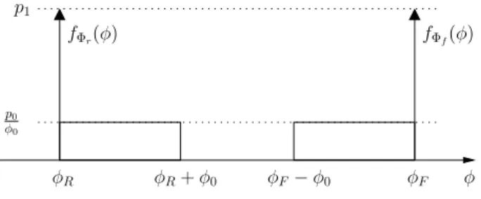
p1 φR fΦr(φ) φR+ φ0 fΦf(φ) φ φF φF− φ0 p0 φ0
Figure 13: PDFs of Φr (left) and Φf (right).
as there is no synchronization between the beacons and the receiver, p1is the probability of determining the correct angle φR as the measured value for Φr, when the beacon enters the angular window. When the beacon emits a 0, the value measured for Φr is not correct; we then assume that its value is uniformly distributed between φRand φR+ φ0. Therefore, if we define δ (x) as the DIRAC delta function, then the PDF
of Φr is given by the following mixture of PDFs
fΦr(φ) = p1δ (φ− φR) + p0U(φR,φR+φ0)(φ) , (10) for φ ∈ [−π, π). After some calculations, we obtain the mean and variance of Φr : µΦr = φR+ p0 φ0 2 , (11) σ2Φr = p0 φ2 0 3 − p 2 0 φ2 0 4 . (12)
Because the configuration is symmetric when the beacon exits the angular window, a similar result yields for Φf
fΦf(φ) = p1δ (φ− φF) + p0U(φF−φ0,φF)(φ) , (13) for φ ∈ [−π, π). The mean and variance of Φf are
µΦf = φF − p0 φ0 2 , (14) σΦ2f = p0 φ2 0 3 − p 2 0 φ2 0 4 . (15)
The PDFs of Φr and Φf are shown in Figure 13. Their expectations have a bias given by ±p0φ20 respectively (see equations (11) and (14)), and their variances are equal. D. Characterization of the estimator Φb
In order to estimate the quality of the beacon angle estimator Φb, we need to evaluate some statistics of Φb, such as its mean and variance.
For two random variables X and Y , we know that E{X + Y} = E{X} + E{Y } (see [30, page 152]). Therefore, according to (11) and (14), the mean of Φb is given by
µΦb =
E{Φr} + E {Φf}
2 =
φR+ φF
2 = φB. (16) The mean of Φb is thus unbiased, despite the fact that both the entering angle Φr and the leaving angle Φf estimators are biased. This justifies the construction of a symmetric receiver and the choice of that particular estimator.
Let us now derive the variance of Φb (see [30, page 155]) σΦ2b = σ2 Φr+ σ 2 Φf + 2C{Φr, Φf} 4 , (17)
where C{Φr, Φf} denotes the covariance of Φrand Φf. If Φr and Φf are uncorrelated, then we have [30, page 155]
σΦ2b= σ2 Φr+ σ 2 Φf 4 = σ2 Φr 2 = σ2 Φf 2 , (18) as σ2 Φr= σ 2
Φf. However, the non correlation or independence of Φr and Φf are questionable in our case, as explained hereafter. As we mentioned earlier, four situations are possible during the angular window defined by φRand φF: (1) no error is encountered, (2) an error occurs for Φr only, (3) an error occurs for Φfonly, or (4) an error occurs for both angles. But, depending on the rotating speed and the code, it is possible to find particular values for the angular window φF − φR for which it is impossible to have an error on Φr and Φf simultaneously (because the codes are deterministic and not random, and the durations between OFF periods are fixed and known). Note that, regardless of the relationship between Φr and Φf, the mean of Φbis always given by equation (16) and Φb remains unbiased. In [32], we have established an upper bound on C {Φr, Φf}, but which over estimates the variance of Φb. Here, we provide a more accurate result. The covariance can be expanded as [30, page 152]
C{Φr, Φf} = E {Φr, Φf} − E {Φr} E {Φf} (19) where E {Φr, Φf} is the joint expectation of Φr and Φf. So, in order to compute this covariance, we should express the joint PDF of Φr and Φf for all possibilities, depending of the angular window and the codes. It can be shown (but this is beyond the scope of this paper2) that the highest value of the variance occurs when no error is possible on Φr and Φf simultaneously (an error on Φr is not balanced by an error on Φf, or vice versa). In that case, the joint PDF is given by
fΦrΦf(φr, φf) = (p1− p0) δ (φr− φR) δ (φf− φF) + p0δ (φr− φR) U(φF−φ0,φF)(φf) + p0δ (φf− φF) U(φR,φR+φ0)(φr)(20) and the joint expectation can be computed as
E{Φr, Φf} = φRφF+ p0(φF− φR)φ0
2 . (21) The substitution of E {Φr, Φf} by its value into equation (19) yields C {Φr, Φf} = p20
φ2 0
4. This result combined with equa-tion (17) finally yields the upper bound of the variance of Φb:
max σΦ2b = p0 φ2
0
6 . (22)
For the parameter values of BeAMS, this variance is 14 % larger than the one given by equation (18), when Φr and Φf are supposed to be uncorrelated.
As expected, the variance is related to the presence of OFF periods in the codes. More precisely, the variance is proportional to the probability of having a zero p0, and to the square of the OFF angle φ0. It is equal to zero if and only if there is no OFF period in the codes. So, this expression establishes that p0and φ0should be kept as small as possible
2The complete demonstration is presented in a technical report [33], available at http://hdl.handle.net/2268/144734
to minimize the effects of the OOK modulation. Note that this variance is an upper bound, since it represents the worst case (no error on Φr and Φf simultaneously), and that this upper bound is the same for all codes (since they all have the same p0 and φ0 by design). In the next section, we discuss these results and compare them to simulated values and to experimental data.
VII. SIMULATED AND EXPERIMENTAL RESULTS
The goal of this section is to provide an error measure for BeAMS. In particular, we want to provide values for the precision (variance) and for the accuracy (bias) of the measured angles.
Our study of the related work has shown that the terms precision, accuracy, and even resolution are sometimes con-fused. This is unfortunate because the knowledge of these characteristics are useful for the data fusion algorithms to take measures into account properly, w.r.t. other measurements. They are also useful to compare systems. Also, some authors characterize their angle measurement systems through a posi-tioning algorithm, and expresses quality results in meters.
It is a well known fact that a positioning process based on angles, regardless of its implementation, depends on the relative configuration of beacons and the robot [10], [14], [15]. So, we believe that an angle measurement system should not be evaluated through a positioning algorithm, unless a common procedure is described and used by everyone. More-over, this evaluation procedure is difficult to implement in practice, and it adds errors due to the setup, especially errors on measurements and on the real location of beacons [26].
In the previous section, we have provided the upper bound for the additional variance on Φbdue to the codes, and showed that the estimator is unbiased. But, in a practical situation, we have to take into account the natural (noise) variance of the system by taking real measurements. This noise is inherent in the hardware, even for a non modulated carrier wave (with no OFF periods). This noise originates from the quartz jitter, rotation jitter, etc, and, to a larger extent, from the receiver jitter at the 0 → 1 and 1 → 0 transitions. From a theoretical point of view, it is acceptable to consider that both noises are independent and, therefore, that the total noise is the sum of the natural noise and σ2
Φb, the power of additional noise induced by the OOK modulation.
The purpose of this section is fourfold: (1) analyze the impact of the code (via the p0 and φ0 parameters) on the variance of Φb, (2) validate the upper bound on the variance of Φb, (3) verify if the artificial noise is independent of the natural noise, and (4) provide values for the precision and accuracy. In order to complete these analyses, simulations and measurements are performed with one beacon for several codes and angular windows.
A. Adding codes for tests only
We have shown that the upper bound of σ2
Φb depends on p0 and φ0. By design, the codes all have the same p0 and φ0. This is an important advantage because this implies that the additional variance is not related to any particular code.
As a consequence, we have to create other codes to observe the influence of p0 and φ0. Also, in order to measure the natural variance, we have to use a special code with no OFF period. So, the codes used for testing purposes are the constant code Ck(no OFF period), the real C5code (“111110111110”), and two variations of code C5 with increasing OFF durations (“11111001111100”, “1111100011111000”). These four codes have a zero symbol probability p0 respectively equal to 0, 1/6,2/7, and3/8, and an OFF angle φ
0 respectively equal to 0, 0.111, 0.222, and 0.333 deg. These variations have been chosen to emphasize the noise due to the OOK modulation, with increasing p0and φ0. In the following section, these four codes are referred to, respectively, as Ck, C5, C5b, and C5c. Note that Ck, C5b, and C5care used for experiments only, but we do not use them in practice.
B. Modifying the angular window
In the last section, we have established the upper bound of σ2
Φb, but we did not provide values of the angular window for which this bound is reached. To establish the mean and variance of Φr and Φf, as well as the mean of Φb, we have assumed the temporal stationarity. This is acceptable as long as the time required for the turret to complete one revolution is not an exact multiple of T0, which is a choice by design. But the variance of Φbover the plane is not uniform. In fact, σ2Φbis invariant to the angle, but it depends on the distance between the beacon and the receiver. We therefore have to understand the relationship between this distance and σ2
Φb by moving a beacon along the radius of a circle centered on the receiver. In practice, the value of the angular window φF − φR depends on the received power and the threshold (see Figure 9). So, for a constant threshold, the angular window decreases if the power curve goes down (less received power), and increases if the power curve goes up (more received power). Then, for a given receiver and optical components, the angular window only depends on the received power. There are two practical ways to modify the received power (or angular window): (1) change the distance between the beacon and the receiver, or (2) change the power emitted by the beacon. But, in any case, the receiver only has access to the angular window via the demodulated signal and it is thus not capable of detecting whether the distance or the emitted power have been modified. In a practical situation, the emitted power of the beacons is expected to be constant, while the distance can change. So we could measure the variance for all possible distances in the working range. However the experiment would be extremely tedious and time-consuming since the number of distances should be huge to appreciate the variations in the measure-ments. So, we choose to modify the emitted power, for a fixed working distance of 1 m. For each code, a hundred different emitted power values were taken in the 4 mW to 150 mW power range to obtain an approximately linear increase of the angular window. These power values and angular windows are values that correspond to distances ranging from 1 m to 6 m. Finally, 1000 angle measurements are taken for each code and power value to compute the mean and variance of Φb. As explained earlier, the receiver is not capable of detecting
Theory Simulations Experiments Φwbias ( deg) Ck 0 0 0 C5 −1.85 10−2 −1.78 10−2 −4.85 10−2 C5b −6.35 10−2 −6.33 10−2 −9.53 10−2 C5c −1.25 10−1 −1.22 10−1 −1.56 10−1 Φbvariance ( deg2) Ck 0 0 3.93 10−3 C5 3.43 10−4 3.36 10−4 5.49 10−3 C5b 2.35 10−3 2.35 10−3 1.00 10−2 C5c 6.94 10−3 6.80 10−3 1.82 10−2
Table II: Comparison of the theoretical, simulated, and experimental values for the biases of Φw, and the maximum variances of Φb, for
the different codes.
whether the distance or the emitted power have been modified and, as a consequence, all the following graphics are plotted with respect to the angular window.
The angular window has to be estimated from the mea-surements. To be more precise and formal, the true angular window φW is defined as φF−φR(see Figure 12). Therefore, we propose an estimator of the angular window given by
Φw= Φf− Φr. (23) The mean of Φw is equal to
µΦw = E{Φf} − E {Φr} = φW − p0φ0. (24) The mean of Φw has a bias given by −p0φ0. But, as the bias of Ck is null since p0 = 0, it is possible to derive φW by taking µΦw for the constant code Ck.
C. Simulator
In order to evaluate our theory about the code statistics, we developed a simulator. The goal is to validate the upper bound on the variance of Φb, as well as the bias of the measured angular window Φw. The four parameters considered by the simulator are the angular window, the code (symbols and durations), the turret period, and the number of turns. The codes, the turret period, and the number of turns are known precisely in our experiments. So, in order to compare the simulated results with the measurements, the angular windows are chosen in the same range as the real values. The simulated angular windows and variances are presented in Figure 14. Simulations confirm our theoretical results as bounds on variances (maximum of the curves) correspond to predicted bounds computed with equation (22). Also, the angu-lar windows have a bias corresponding to values predicted by equation (24) (the numerical values are given in Table II). The simulator confirms our theoretical results about the variance added by the codes. However, the simulator does not take into account the natural noise of the system. So we have to use the real system to measure this natural noise. The results are presented in the next section.
D. Experiments
The angular windows for each code are shown in the top plot of Figure 15 and the values of the biases are given in Table II. As expected, the curves are linear with the angular window. But the biases observed for the angular windows are
Ck C5 C5b C5c 5 5.5 6 6.5 7 5 5.5 6 6.5 7 Mean angular windo w (deg )
Angular window (deg) Ck C5 C5b C5c 0 0.002 0.004 0.006 0.008 0.01 0.012 0.014 0.016 0.018 5 5.5 6 6.5 7 V ariance (deg 2)
Angular window (deg)
Figure 14: Results of simulations: values for the mean of the angular window Φw(top), and for the variance of the beacon angular position
Φb(bottom).
larger (in absolute value) than the theoretical biases. On the other hand, they increase with p0and φ0, and the increments between the experimental biases are consistent with the theory. The variances of the measurements for Φbare shown in the bottom plot of Figure 15. One can observe that the variance increases with p0and φ0, respectively for Ck(the lowest), C5, C5b, and C5c (the highest), for all angular windows. One also sees large variations, especially for C5band C5c. This indicates that a dependency between Φr and Φf in function of the angular window exists. Examining the variances of Φr and Φf separately helps in this analysis (see Figure 16). Whereas Φr and Φf variances are quasi linear with respect to the angular window, Φb is not linear despite the fact that the estimator Φb is a linear function of the estimators Φr and Φf. This confirms that a statistical relationship exists between Φr and Φf.
Of course, there is a difference with the simulations since the measurements include the natural noise of the system and, as a result, the variances of the measurements are higher than the simulations. If the artificial noise due to the codes was independent of the natural noise, the measured variances could be obtained by adding the natural noise (measured with Ck) to the simulated variances. However, this is not the case
Ck C5 C5b C5c 5 5.5 6 6.5 7 5 5.5 6 6.5 7 Mean angular windo w (deg )
Angular window (deg) Ck C5 C5b C5c 0 0.002 0.004 0.006 0.008 0.01 0.012 0.014 0.016 0.018 5 5.5 6 6.5 7 V ariance (deg 2)
Angular window (deg)
Figure 15: Results of measurements: values for the mean of the angular window Φw(top), and for the variance of the beacon angular
position Φb(bottom).
since the variances obtained with this hypothesis (not shown here) still remain lower (but close) than the real variances. This result indicates that the natural and artificial noises are not independent, and that the real noise is higher than their sum. But, despite this discrepancy, the general shape of the simulated and experimental curves is similar. In particular, the large variations in the curves, the locations of the extrema, as well as their relative distances match our experiments perfectly (compare bottom plots of Figure 14 and Figure 15). Finally, note that we are interested in finding the variance of the measured angles in BeAMS, in the whole working range. The maximum of the curve measured for C5yields a variance equal to 5.49 10−3deg2, or equivalently a standard deviation equal to 7.41 10−2deg.
E. Discussions of the experiments
Our simulator provides values for the variances of Φb and biases of the angular window that match that of our theo-retical model. However, they are some discrepancies between the experimental results and the theoretical bound. Amongst these discrepancies, the hypothesis that the natural variance is independent of the variance added by a code, as implemented
Ck C5 C5b C5c 0 0.005 0.01 0.015 0.02 0.025 0.03 0.035 0.04 5 5.5 6 6.5 7 V ariance (deg 2)
Angular window (deg) Ck C5 C5b C5c 0 0.005 0.01 0.015 0.02 0.025 0.03 0.035 0.04 5 5.5 6 6.5 7 V ariance (deg 2)
Angular window (deg)
Figure 16: Results of measurements: variance of the beacon angular rising Φr (top) and falling Φf (bottom) edges.
in the simulator, is most subject to questioning. The reason for this is as follows. A detailed analysis of the receiver hardware shows the presence of an “Automatic Gain Control” (AGC) loop between the input and the demodulator. Typically, the gain is set to a high value when no signal is present for a “long time”, resulting in a very noisy first transition (Φr in our case). This gain then decreases over time, resulting in sharper transitions (especially the last one, Φf in our case). This characteristic is clearly identifiable from the variances of Φr and Φf for a non modulated signal Ck (see Figure 16). It appears that the gain value depends on the past values of the received signal and the duration of the OFF periods, and this produces a non constant natural variance over time. So, we have to consider this effect in tightening the agreement between theoretical and practical results. But it is no small task to consider this effect because it relates to the hardware. Also, we have to consider another effect of the receiver hardware. In Section VI-A, we supposed that the received signal Ri could be modeled has the logical AND between the emitted signal Ei and R0. However, it is not sure that a short leading or tailing burst (shorter than a bit) could trigger the receiver (see for example R2, and R3 in Figure 12). This has the effect of virtually increasing the OFF period