Synchronization with partial state feedback on SO(n),

Af- ter the Comment Resource was published the Annotation Client notifies the Semantic Pingback Service by sending a pingback request with the Comment Resource as source and

In this paper, we consider discrete event systems divided in a main system and a secondary system such that the inner dynamics of each system is ruled by standard synchronizations

Key words: networked/embedded control systems, state dependent sampling, self-triggered control, Lyapunov-Razumikhin, linear matrix inequality, convex polytope, exponential

FFT reduces the spacing between the orthogonal sub carriers. Two sinusoids of the same parameters can become orthogonal to each other by separating them far apart in frequency domain

The algorithm is composed of an initialization stage (see Section 4.1) followed by three main stages as summarized in Figure 3: (i) the CTS stage, which uses not only STF but also

In this paper, we consider discrete event systems divided in a main system and a secondary system such that the inner dynamics of each system is ruled by standard synchronizations

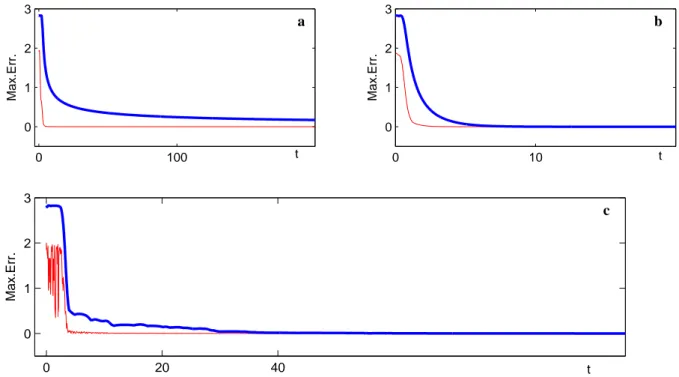
A high gain state observer for a class of systems similar to (1) has been proposed in Farza et al. [1999] considered a stabilization problem for a class of non uniformly observ-

First the nominal case is considered and a control law is designed, then an observer reconstruct the current delivered to the load and the output voltage, finally, these two parts