Idiosyncratic Consumption Risk and the Cross-Section of Asset Returns

(1)

Montréal

Série Scientifique

Scientific Series

2002s-11

Idiosyncratic Consumption

Risk and the Cross-Section of

Asset Returns

(2)

CIRANO

Le CIRANO est un organisme sans but lucratif constitué en vertu de la Loi des compagnies du Québec. Le financement de son infrastructure et de ses activités de recherche provient des cotisations de ses organisations-membres, d’une subvention d’infrastructure du ministère de la Recherche, de la Science et de la Technologie, de même que des subventions et mandats obtenus par ses équipes de recherche.

CIRANO is a private non-profit organization incorporated under the Québec Companies Act. Its infrastructure and research activities are funded through fees paid by member organizations, an infrastructure grant from the Ministère de la Recherche, de la Science et de la Technologie, and grants and research mandates obtained by its research teams.

Les organisations-partenaires / The Partner Organizations •École des Hautes Études Commerciales

•École Polytechnique de Montréal •Université Concordia

•Université de Montréal

•Université du Québec à Montréal •Université Laval

•Université McGill

•Ministère des Finances du Québec •MRST

•Alcan inc. •AXA Canada •Banque du Canada

•Banque Laurentienne du Canada •Banque Nationale du Canada •Banque Royale du Canada •Bell Canada

•Bombardier •Bourse de Montréal

•Développement des ressources humaines Canada (DRHC) •Fédération des caisses Desjardins du Québec

•Hydro-Québec •Industrie Canada

•Pratt & Whitney Canada Inc. •Raymond Chabot Grant Thornton •Ville de Montréal

Short sections may be quoted without explicit permission, if full credit, including © notice, is given to the source.

ISSN 1198-8177

Les cahiers de la série scientifique (CS) visent à rendre accessibles des résultats de recherche effectuée au CIRANO afin de susciter échanges et commentaires. Ces cahiers sont écrits dans le style des publications scientifiques. Les idées et les opinions émises sont sous l’unique responsabilité des auteurs et ne représentent pas nécessairement les positions du CIRANO ou de ses partenaires.

This paper presents research carried out at CIRANO and aims at encouraging discussion and comment. The observations and viewpoints expressed are the sole responsibility of the authors. They do not necessarily represent positions of CIRANO or its partners.

(3)

Idiosyncratic Consumption Risk

and the Cross-Section of Asset Returns

*

Kris Jacobs

†

and Kevin Q. Wang

‡

First version: Novembre 2000 This revision: August 2001

Résumé / Abstract

Cet article analyse l’importance du risque idiosyncratique de la consommation individuelle pour la variance transversale des rendements moyens des actifs et des obligations. Lorsque l’on n’attribue pas de prix au risque idiosyncratique de la consommation individuelle, le seul facteur d’évaluation dans une économie à plusieurs horizons est le taux de croissance de la consommation agrégée. Nous montrons que la variance transversale de la croissance de la consommation est également un facteur dont le prix est déterminé. Ceci démontre que les consommateurs ne sont pas complètement assurés contre le risque idiosyncratique de la consommation et que les rendements des actifs reflètent leurs efforts à réduire leur exposition à ce risque. Pour la période considérée, nous trouvons que le modèle d’évaluation d’actifs à deux facteurs basés sur la consommation donne de meilleurs résultats que le CAPM. De plus, la performance empirique du modèle se compare favorablement avec celle du modèle à trois facteurs de Fama-French. Par ailleurs, en présence du facteur de marché et des facteurs taille et ratio valeur comptable/cours, les deux facteurs basés sur la consommation conservent leur pouvoir explicatif. Combiné aux résultats de Lettau et Ludvigson (2000), ces résultats indiquent que l’évaluation d’actifs à partir de la consommation sert à expliquer l’intégralité des rendements d’actifs.

This paper investigates the importance of idiosyncratic consumption risk for the cross-sectional variation in average returns on stocks and bonds. If idiosyncratic consumption risk is not priced, the only pricing factor in a multiperiod economy is the rate of aggregate consumption growth. We offer evidence that the cross-sectional variance of consumption growth is also a priced factor. This demonstrates that consumers are not fully insured against idiosyncratic consumption risk, and that asset returns reflect their attempts to reduce their exposure to this risk. We find that over the sample period the resulting two-factor consumption-based asset pricing model significantly outperforms the CAPM. The model’s empirical performance also compares favorably with that of the Fama-French three-factor model. Moreover, in the presence of the market factor and the size and book-to-market factors, the two consumption based factors retain explanatory power. Together with the results of Lettau and Ludvigson (2000), these findings indicate that consumption-based asset pricing is relevant for explaining the cross-section of asset returns.

JEL: G12

Mots clés : évaluation d’actifs transversale, modèle basé sur la consommation, risque de consommation

idiosyncratique, marchés incomplets, erreur de mesure

Keywords: cross-sectional asset pricing; consumption-based model; idiosyncratic consumption risk;

incomplete markets; measurement error

*

Jacobs acknowledges FCAR of Québec and SSHRC of Canada for financial support. Wang acknowledges the Connaught Fund at the University of Toronto for financial support. We are very grateful to Eugene Fama and Raymond Kan for providing us with the asset return data. We would also like to thank Joao Cocco, Francisco Gomes, Raymond Kan, Tom McCurdy, Sergei Sarkissian and Raman Uppal for helpful comments. Correspondence to: Kris Jacobs, Faculty of Management, McGill University, 1001 Sherbrooke Street West, Montreal, Canada H3A 1G5; Tel: (514) 398-4025; Fax: (514) 398-3876; E-mail: Jacobs@Management.McGill.CA.

(4)

1 Introduction

If agents manage to perfectly insure themselves against idiosyncratic consumption risk, the only relevant pricing factor in a standard multiperiod asset pricing model without frictions is the growth rate of aggregate consumption. However, the workhorse representative-agent consumption-based asset pricing model (CCAPM) that reßects this allocation is not able to match important aspects of the distribution of historical asset returns, such as the risk premium on the market portfolio. Its performance in a cross-sectional context is weak and has certainly not been suﬃciently satisfactory to threaten alternative cross-sectional models such as the Capital Asset Pricing Model (CAPM).1

However, if agents cannot perfectly insure themselves against idiosyncratic consumption risk,2 _{factors other than aggregate consumption growth become relevant to price assets.}

Un-der this assumption, all higher moments of the cross-sectional distribution of consumption growth are relevant pricing factors. Researchers have long realized that changes in these moments may be of critical importance to explain changes in asset prices (see Mehra and Prescott (1985)). Building on this insight, a number of studies have investigated the impor-tance of market incompleteness for the equity premium puzzle and the risk-free rate puzzle (see Telmer (1993), Constantinides and Duﬃe (1996), Heaton and Lucas (1996), Jacobs (1999), Vissing-Jorgensen (2000), Cogley (1999), Brav, Constantinides and Geczy (1999) and Balduzzi and Yao (2000)). These studies provide mixed evidence on market incomplete-ness and the literature has not yet fully matured, but it is a safe conclusion that models with uninsurable idiosyncratic consumption risk and potentially limited market participation stand a better chance to explain the data than standard representative-agent models.

This paper further investigates the importance of uninsurable idiosyncratic risk by ex-amining its importance for the cross-section of asset returns. In principle, one can investi-gate the set of intertemporal restrictions associated with the cross-section of returns using a number of alternative procedures. For instance, one can specify a utility function and use a distributional assumption to obtain a pricing kernel that is a well-deÞned nonlinear parametric transformation of consumption-based pricing factors. Constantinides and Duﬃe (1996) use such a setup with constant relative risk aversion and a lognormality assumption on idiosyncratic income shocks. They obtain two consumption-based pricing factors,

rep-1_{A recent paper by Lettau and Ludvigson (2000) demonstrates that consumption-based models can} challenge the CAPM along certain dimensions. This research is discussed below.

2_{At this point, it is important to elaborate on the terminology used in this paper in order to avoid} confusion. In the literature on the CAPM, standard terminology splits up the risk of an individual asset into market risk and idiosyncratic risk. In this paper the focus is on idiosyncratic risk for an individual consumer. It is standard in the incomplete markets literature to refer to this risk as “idiosyncratic income risk” or “idiosyncratic risk”. In this paper we do not investigate a full general equilibrium model but focus exclusively on equilibrium intertemporal consumption allocations. Therefore we refer to this idiosyncratic risk as “idiosyncratic consumption risk”. This terminology is slightly unsatisfactory but preferable to the use of “idiosyncratic risk”, which could be confused with the terminology used in the context of the CAPM.

(5)

resenting the rate of consumption growth and the cross-sectional variance of the logarithm of consumption growth (consumption dispersion). Alternatively, Cogley’s (1999) analysis illustrates the importance of additional pricing factors representing higher moments of the cross-sectional distribution of consumption growth. We follow a slightly diﬀerent approach, designed to keep the econometric analysis relatively simple and to allow us to conduct a search over diﬀerent speciÞcations. To do this, we investigate a variety of pricing kernels that are linear in consumption growth and consumption dispersion.

We investigate the empirical performance of these pricing kernels using household con-sumption data from the Consumer Expenditure Survey (CEX). We examine the performance of the pricing kernels using four different datasets. The Þrst two datasets use data on non-durables and services consumption. The difference between the two samples is that the Þrst dataset is based on all households that fulÞll certain selection criteria, whereas the sec-ond dataset only contains households that hold assets. The difference between the third and the fourth dataset is also based on whether the household holds assets, but both these datasets use data on total consumption. Moreover, for each of the resulting four datasets, we construct the consumption-based pricing factors in different ways. First, we compute average consumption growth and consumption dispersion by using data on individual house-hold consumption. However, we know that the presence of measurement error is a serious problem when using household consumption data. To deal with this problem, we recon-struct the consumption-based factors using data on the consumption of a synthetic cohort of individuals, rather than a single individual.

We Þnd that regardless of the dataset, consumption dispersion is a priced factor, in-dicating the relevance of uninsurable consumption risk for asset returns. The sign of the priced consumption dispersion factor depends on the dataset. This is of interest because for idiosyncratic consumption risk to help resolve the equity premium puzzle, it has to be the case that consumption dispersion is larger in recessions. Intuitively this leads to an increase in the risk faced by an individual agent, and this leads to a larger risk premium to induce investors to hold risky assets. However, we Þnd that whereas the Þrst consumption-based factor (average consumption growth) always displays the expected positive correlation with returns, we only obtain robust estimates of negative correlation between returns and con-sumption dispersion when considering data on total concon-sumption, and only when limiting the sample to asset holders.

This Þnding is not surprising. Other studies also conclude that the distribution of consumption for assetholders is diﬀerent from that for non-assetholders. Moreover, durable consumption is the most cyclical component of individual consumption. Therefore, the data simply tell us that the less wealthy cut back a lot more than the wealthy on their consumption in recessions and make up for it in expansions. However, because it is relatively harder to cut back on nondurable consumption, they implement this through their expenditures on durable consumption. Finally, it must be noted that these Þndings are obtained using pricing factors constructed from cohort data. When using individual data, estimates are

(6)

often insigniÞcant and not very robust. This Þnding is consistent with the Þndings of Brav, Constantinides and Geczy (1999) in the context of the equity premium puzzle.

To evaluate the signiÞcance of these Þndings, we investigate their robustness and compare the performance of the pricing factors against a number of alternatives. We Þnd that the two-factor consumption-based model (with consumption growth and consumption dispersion as factors) signiÞcantly outperforms the CAPM and the one-factor consumption based model over the sample period under consideration. Moreover, the empirical performance of the two-factor consumption-based model also compares favorably with that of the three-factor model proposed by Fama and French (1993). Finally, we investigate pricing kernels that combine size and book-to-market factors and/or the CAPM factor with the consumption-based factors. It is shown that even after accounting for these alternative pricing factors, the consumption-based factors are estimated signiÞcantly in the pricing equation.

2 Idiosyncratic Consumption Risk and the Cross-Section

of Asset Returns

Following the seminal contributions by Lucas (1978) and Breeden (1979), a number of pa-pers have conducted empirical investigations of representative-agent consumption-based as-set pricing models. Even though these models have a wide range of empirical implications, a large part of the literature has a rather limited focus. In fact, much of the empirical research on consumption-based models has focused exclusively on the returns on a riskless asset and the market index, leading to the so-called equity premium and riskfree rate puzzles.3 _A

small number of papers study the performance of the consumption-based model in a cross-sectional context. Mankiw and Shapiro (1986), Breeden, Gibbons and Litzenberger (1989) and Cochrane (1996) conclude that the performance of the consumption-based model is un-satisfactory and that the consumption-based model performs no better than the CAPM. However, more recently Lettau and Ludvigson (2000) show that those negative conclusions about the performance of the consumption-based model are due to the fact that those em-pirical studies investigate an unconditional linear factor model. When investigating a con-ditional factor model, the model’s performance is about as good as that of the three-factor Fama-French model, when using a speciÞc conditioning variable that is suggested by theory. Campbell and Cochrane (2000) provide an explanation for why consumption-based asset pricing models perform better conditionally than unconditionally.

This paper reaﬃrms that consumption-based asset pricing models are valuable for the study of the cross-section of asset returns. It shows that this is the case even when studying

3_{Hansen and Singleton (1982,1984), Mehra and Prescott (1985) and Grossman, Melino and Shiller (1985)} focus exclusively on a riskless and a risky asset. Other papers such as Hansen and Singleton (1983) and Epstein and Zin (1991) focus on the equity premium puzzle but investigate some other risky assets. However, none of these papers speciÞcally focuses on the cross-section of returns.

(7)

unconditional models, as opposed to the conditional models studied by Lettau and Ludvigson (2000). The key to this Þnding is that one has to move away from the rigid construction of a representative agent economy, which implies the irrelevance of idiosyncratic consumption risk. To appreciate the importance of this modeling approach, it is instructive to review the importance of complete markets and the representative agent assumption for the equity premium and riskfree rate puzzles.4 _{The complete markets assumption is critical for the}

rep-resentative agent model. Individual agents that are faced with a complete markets structure can insure themselves against idiosyncratic consumption risk. As a consequence, the prices of assets in the economy are equivalent to the prices in a closely related representative agent economy.

Whereas the complete markets assumption is a convenient modeling technique, casual observation as well as empirical testing has convinced most researchers that it is not very realistic (see Cochrane (1991), Mace (1991), Hayashi, Altonji and Kotlikoﬀ (1994)). It is therefore not surprising that a growing number of studies investigate to what extent market incompleteness is of interest to explain the empirical rejections of the consumption-based models. A number of these studies investigate this issue by using simulation-based models. Whereas early studies by Telmer (1993) and Heaton and Lucas (1996) do not manage to generate large enough risk premia for most realistic parameterizations of the economy, later studies by Telmer, Storesletten and Yaron (1997) and Constantinides, Donaldson and Mehra (1998) have managed to generate larger risk premia under the assumption that idiosyncratic shocks are fairly persistent. A number of other studies (Jacobs (1999), Vissing-Jorgensen (2000), Cogley (1999), Brav, Constantinides and Geczy (1999) and Balduzzi and Yao (2000)) have analyzed market incompleteness from another perspective, by investigating Euler equa-tions that hold even if markets are incomplete. Sarkissian (1998) analyzes incomplete risk sharing between countries. The test results in these papers are mixed, but a robust con-clusion is that risk aversion implied by restrictions from incomplete markets is lower than risk aversion implied by representative agent models. Taken together, the Þndings in the literature on market incompleteness seem to indicate that accounting for idiosyncratic con-sumption risk has at least some potential to explain the structure of asset returns.

Because models with incomplete markets have had some success explaining the equity premium and risk-free rate puzzles, it seems therefore natural to investigate if they can

4_{The literature contains other attempts to explain the equity premium puzzle and riskfree rate puzzle.} A number of papers have focused on the importance of time aggregation (see Grossman, Melino and Shiller (1987) and Heaton (1993)). Also, an extensive literature has studied the modeling of alternative preferences for the representative agent (see Abel (1990), Campbell and Cochrane (1999), Cochrane and Hansen (1992), Constantinides (1990), Detemple and Zapatero (1990), Epstein and Zin (1991), Ferson and Constantinides (1991), Heaton (1995), and Sundaresan (1989)) . These approaches alleviate some of the problems with representative agent models and it is possible that they would also improve the cross-sectional performance of consumption-based models. See Kocherlakota (1996), Campbell, Lo and MacKinlay (1997) and Cochrane (2001) for overviews of this literature.

(8)

be used to explain a wider cross-section of asset returns. In cross-sectional asset pricing, the Capital Asset Pricing Model (CAPM) is the dominant paradigm. It is therefore a natural benchmark to evaluate the performance of a consumption-based model with market incompleteness. Ferson (1995) and Cochrane (1996, 2001) show that the traditional form of factor pricing models such as the CAPM can be implemented by using the intertemporal optimality condition

E[MtRj,t|Ωt−1] = 1 (1)

where Mt is the pricing kernel, Rj,t is the return on asset j at time t and Ωt−1 is the

information set available to the econometrician at time t_{− 1. For the CAPM, the pricing} kernel Mt is speciÞed as follows

Mt= β0+ β1RM,t (2)

where RM,t is the return on the market portfolio at time t. We now outline a framework

that allows us to compare the performance of a pricing kernel that accounts for idiosyncratic consumption risk with the performance of the CAPM as evaluated in (1) and (2). The intertemporal optimality condition associated with individual i’s investment in asset j implies that

E[Mi,t(cgi,t)Rj,t|Ωt−1] = 1 (3)

where the pricing kernel Mi,twhich is indexed by individual i depends on consumption growth

cgi,t = ci,t/ci,t−1 in the context of a consumption-based asset pricing model. Averaging this

orthogonality condition for asset j over all N consumers we get E[(1/N )

N

X

i=1

Mi,t(cgi,t)Rj,t|Ωt−1] = 1 (4)

The pricing kernel in (4) will also be referred to as Mt = (1/N )PNi=1Mi,t(cgi,t).

Eval-uating the performance of this kernel in the cross-section can then be accomplished by specifying the underlying structure of the economy. For instance, if individual consumers have time-separable constant relative risk aversion (TS-CRRA), this average intertemporal Euler equation for consumer i and asset j is

E[(1/N ) e−θ

N

X

i=1

(cgi,t)−αRj,t|Ωt−1] = 1 (5)

where α is the rate of relative risk aversion and θ is the rate of time preference.

Constantinides and Duﬃe (1996, henceforth CD) clearly highlight the importance of consumption dispersion under market incompleteness. Using a TS-CRRA speciÞcation, they specify an economy that leads to an Euler equation that speciÞes explicitly how the pricing

(9)

kernel depends on the moments of the cross-sectional distribution of consumption growth. SpeciÞcally, their economy yields the following intertemporal Euler equation

E[e−θ(ct/ct−1)−αexp(

α(α + 1)

2 y

2

t)Rj,t|Ωt−1] = 1 (6)

where ct is aggregate consumption at time t and yt2 can be interpreted as the variance of

the cross-sectional distribution of log[(ci,t/ct)/(ci,t−1/ct−1)].5 Cogley (1999) uses a diﬀerent

approach to show that in general the pricing kernel will depend on all moments of the cross-sectional distribution. When omitting moments higher than the second moment and specializing the analysis to a TS-CRRA utility function, he shows that one obtains an Euler equation similar to (6).

The cross-section of asset returns can be analyzed by using the generalized method of moments to evaluate (5) and (6) directly. However, the disadvantage of this approach is that the resulting econometric problem is highly nonlinear. This may complicate the optimization and the comparison with the benchmark CAPM because of the existence of local optima. We therefore use a diﬀerent approach inspired by Cochrane (1996). It is clear from Cogley (1999) that with incomplete markets the pricing kernel depends on the cross-sectional mo-ments of consumption growth.6 Moreover, because it is diﬃcult to estimate higher moments precisely, it is preferable to limit attention to the Þrst two moments. The precise nature of the relationship between the pricing kernel and these moments depends on the speciÞcation of the utility function. We therefore assume that the pricing kernel depends in a simple linear way on the Þrst two cross-sectional moments of consumption growth7

Mt = β0+ β1mcgt+ β2vcgt (7)

where mcgt = (1/N )PNi=1(cgi,t) and vcgt = (1/N )PNi=1(cgi,t− mcgt)2. Implicitly of course

this linear kernel corresponds to some utility function. If this utility function is a poor approximation of reality, this will aﬀect the performance of the pricing kernel negatively.8

5_{Balduzzi and Yao (2000) use a different setup which leads to a different Euler equation. In their economy} the second factor is not the cross-sectional variance of log consumption growth, but the difference of the variance in cross-sectional consumption. They also use this kernel to study the cross-section of asset returns. 6_{It must be noted that market incompleteness is not a necessary condition for the higher moments of} consumption growth to enter the pricing kernel. For example, investor heterogeneity can have similar effects (Dumas (1989)). Basak and Cuoco (1989) explicitly characterize the cross-sectional distribution of consumption in a model with market incompleteness and investor heterogeneity.

7_{Heaton and Lucas (2000) also investigate linear pricing kernels with measures of idiosyncratic income} risk as pricing factors. They Þnd that the existence of entrepreneurial income risk has a signiÞcant inßuence on asset returns.

8_{Notice however that the linear kernel can be seen as a Taylor series approximation to any utility function} as long as one does not impose restrictions emanating from an underlying utility function on the coeﬃcients in (7).

(10)

We also compare the performance of the consumption-based factors to a benchmark other than the CAPM. A logical choice is to make a comparison with the size and book-to-market factors proposed by Fama and French (1992, 1993). We use the kernel for the Fama-French three factor model

Mt = β0+ β1RM,t+ β2SM Bt+ β3HM Lt (8)

where SM Bt is the size factor and HM Lt is the book-to-market factor. To evaluate the

relative performance of the consumption-based factors compared to the Fama-French factors, we investigate a number of kernels where we interact the consumption-based factors with the size and/or book-to-market and/or market factors. These kernels are described in more detail in the tables.

3 Data Description

This section discusses three diﬀerent issues related to data construction. The empirical procedure is implemented as follows. First, consumption data are used to construct pricing factors that estimate the Þrst and the second moments of the cross-sectional distribution of consumption growth. The approach used to construct the consumption data is described in Section 3.2. In a second stage, these pricing factors are taken as given in an econometric investigation of the intertemporal relation (1) for a wide cross-section of asset returns. This cross-section of asset returns is described in Section 3.1. It must be noted at this point that the uncertainty involved in constructing the pricing factors is neglected in this econometric analysis. A Þnal critical issue related to data construction is the construction of synthetic cohorts described in Section 3.3. The motivation for using synthetic cohorts is the well-documented existence of substantial measurement error in household consumption data. Finally, Section 3.4 discusses at length the statistical properties of the four diﬀerent samples used in the analysis and the factors used in the pricing equation.

3.1 Asset Return Data

We use a set of test portfolios that includes the twenty-Þve size and book-to-market portfolios of Fama and French (1993), a long term government bond, a long term corporate bond, and the 3-month Treasury bill rate. The data are quarterly, and they are constructed from the corresponding monthly data, ranging from April 1984 to December 1995. The Fama-French portfolios are now widely used. They are value-weighted portfolios of stocks listed on the NYSE, AMEX, and NASDAQ. These portfolios are sorted on Þrm size and book-to-market equity and exhibit strong cross-sectional dispersion in average returns. (For more details on the portfolios, see Fama and French (1993)). For the bond returns, we use the total return on Treasury bonds (the CRSP variable GBTRET), the total return on long term corporate bonds (the CRSP variable CBTRET), and the three-month T-bill rate. For the market

(11)

portfolio, we use the CRSP value-weighted portfolio of stocks listed on NYSE, AMEX, and NASDAQ that Fama and French use to proxy for the market portfolio.9 _{Also included in our}

empirical tests are the size (SMB) and book-to-market (HML) factors of Fama and French. All the variables are in real terms.

Descriptive statistics for the test portfolios are given in Table I. An important observation is that for the stock portfolios, which are sorted according to size and book-to-market, the pattern of average returns is very different from the one documented in Fama and French (1993). This difference is due to the different sample period. Most importantly, for the sample under consideration in this paper, Table I conÞrms the observation of Cochrane (2001, p. 438) that the size effect has disappeared in the eighties.

3.2 Consumption Data

To construct the pricing factors, we use data on household consumption from the Consumer Expenditure Survey (CEX). The CEX data have been used by a number of researchers to analyze the importance of idiosyncratic consumption risk for the equity premium puzzle (e.g. see Brav, Constantinides and Geczy (1999), Vissing-Jorgensen (2000), Cogley (1999) and Balduzzi and Yao (2000)). Balduzzi and Yao (2000) also present an analysis of cross-sectional pricing using their (diﬀerent) pricing kernel. The advantage of the CEX is that it provides a measure of total consumption, unlike other datasets such as the Panel Study of Income Dynamics. The CEX is not a genuine panel dataset, but a series of cross-sections with a limited time dimension. However, in the context of the exercise proposed in this paper, this is not necessarily a very serious problem, because at each time we simply use every available cross-section to construct cross-sectional moments.

We construct the pricing factors using two measures of household consumption. The Þrst measure corresponds to nondurable consumption plus services. The second measure corre-sponds to total consumption, including durable consumption. The use of data on durable consumption is fairly common in the consumption literature, and its importance is well rec-ognized because durable consumption has diﬀerent stochastic properties from nondurable consumption (e.g. see Christiano, Eichenbaum and Marshall (1991), Darby (1975), Eichen-baum and Hansen (1990), Mankiw (1985), Ogaki and Reinhart (1998), Sargent (1978) and Startz (1989)). However, the modeling of durable consumption in this paper is nonstandard, largely because of data constraints. In the time-series literature on durable consumption, the starting point is a time series of the stock of durable goods. Consumption of durable

9_{We follow a long tradition in the Þnance literature by measuring R}

M,t using the return on publicly listed stocks. A large number of studies have debated whether to include the return on human capital in this construction (see Mayers (1972), Roll (1977), Fama and Schwert (1977), Campbell (1996), Jagannathan and Wang (1996) and Lettau and Ludvigson (2000)). We do not analyze this issue, because our primary motivation for studying the CAPM here is to Þnd an appropriate benchmark for the performance of our consumption-based model, and not the appropriate speciÞcation of the market return.

(12)

goods is then usually modeled as a distributed lag in this stock variable. Because studies based on household data are based on reports on expenditures instead of a stock of durable goods, we proceed in a diﬀerent way. Hayashi (1985) models durable consumption us-ing household data by specifyus-ing a distributed lag in expenditure on durable goods.10 _In

this paper, we model consumption of total expenditures, implicitly treating nondurable and durable consumption as perfect substitutes. This approach is motivated by the need to oﬀer alternatives to the CAPM that have a small number of factors. By modeling durable and nondurable consumption separately, one would introduce separate factors for each consump-tion category. By modeling consumpconsump-tion as a distributed lag of past expenditures, lagged durable consumption growth would show up as an extra factor.11

Even though participants in the CEX are interviewed on a quarterly basis, one can in principle construct consumption data for diﬀerent frequencies. After each quarter, par-ticipants are asked detailed questions about their consumption patterns in the past three months. It is possible to construct monthly consumption data from these interviews. How-ever, the resulting time series is fairly constant over a three-month period and then jumps to another level (see also Vissing-Jorgensen (2000) on this issue). Therefore, we follow most of the available literature that uses the CEX and construct quarterly data (see Brav, Constan-tinides and Geczy (1999), Vissing-Jorgensen (2000) and Cogley (1999)). The CEX data are available from 1984 to 1995. Because we use data on consumption growth, the Þrst available quarter is therefore the second quarter of 1984. Also, because of a data matching problem, we cannot use data on the Þrst quarter of 1986. Moreover, several indicators revealed low data quality for the last quarter available (the fourth quarter of 1995). We therefore exclude this quarter. This leaves us with 45 quarterly observations.

Another issue that deserves discussion is family composition. The CEX reports con-sumption for the household unit. This complicates the analysis, because as a result one of the factors driving cross-sectional and time-series diﬀerences in consumption is changes and diﬀerences in family size. There are several ways to correct for this when estimating intertemporal optimality conditions in the presence of idiosyncratic consumption risk. First, one can include a function of family size in the deÞnition of consumption in period t. This is useful when directly analyzing the Euler equation (5) (see Jacobs (1999)). An second alternative is to simply divide household consumption by the number of members of the household. Whereas this is of course done when using aggregate per capita consumption

10_{The use of expenditure data is problematic to the extent that large expenditures are made at one point} in time on durable goods that yield consumption services at some other point in time. It must be noted in this respect that to the extent that consumers purchase durable goods on credit, the match between expenditure and consumption is probably rather good.

11_{It is clear that because of data constraints the modeling of durable goods consumption is subject to} diﬀerent problems than the ones we encounter when using time-series data. If as a result of this the link between the resulting pricing factors in (7) and the consumer’s utility function is unconvincing, one can also interpret the factors as attempting to capture business cycles in expenditures by consumers.

(13)

data, the issue is less straightforward when using household data because the data reveal that household consumption is a complicated nonlinear function of household size. A third alternative is to correct for family size using a given scale which is used in the literature or estimated from the data. The Þrst technique is not applicable in the context of this paper, be-cause we do not analyze the intertemporal optimality conditions directly. We Þrst construct the factors and then use those factors in a regression framework. We attempted to correct for household size using the second and third alternatives. Because this does not make a diﬀerence, we present results using household consumption as the unit of observation.

A Þnal robustness issue is the presence of seasonalities. It is well known that season-alities are present in consumption data and that they are important for asset pricing (see Miron (1986) and Ferson and Harvey (1992)). When inspecting the raw CEX household consumption data, seasonalities seem to be even more pronounced than for quarterly NIPA data. The most obvious manifestation of this Þnding is the well known dent in consump-tion in the Þrst quarter. Reported results do not adjust for seasonality, in accordance with other papers that use the CEX (see Attanasio and Weber (1995), Brav, Constantinides and Geczy (1999), Vissing-Jorgensen (2000), Cogley (1999) and Balduzzi and Yao (2000)). We performed a robustness exercise by controlling for seasonality using the census X11 method as implemented in EVIEWS. Even though the resulting seasonal adjustment factors are nonnegligible (as is the case for NIPA data), this does not aﬀect test results.

In the expanding literature that investigates the equity premium puzzle using disaggre-gate data, one important conclusion is that asset market participation is of great importance. It seems that the consumption patterns of households that hold assets are more consistent with economic theory. One of the strengths of the CEX is that it contains a wealth of information on asset holdings. We therefore conduct our analysis for a sample that contains all households, but also for a sample that only contains assetholders. Given the wealth of asset information in the CEX, several selection criteria can be used and existing studies have constructed widely diﬀerent samples of assetholders. For example, the CEX reports data on holdings of checking and savings accounts, bonds and stocks, and participation in private and public pension plans. Moreover, the CEX reports data on the income received from a certain asset (a ßow variable) as well as the holdings of the same asset (a stock variable). Also, in the CEX all these questions are asked in reference to two points in time, the Þrst and the last (Þfth) quarter that the households are in the sample. To determine which households are assetholders, we use the answer referring to the Þrst quarter.

Ideally we would like to construct a sample of individuals who hold any type of asset and also a sample of individuals who hold stocks. Unfortunately, this is not possible because the CEX does not ask a direct question on whether an individual holds stocks either directly or indirectly through a pension plan. We therefore proceed to construct a sample of households who are very likely to hold stocks. It consists of households that report the existence of at least one of the following: (i) holdings of stocks or bonds, (ii) dividend income, and/or (iii) contributions to an IRA. It is clear that this is an imperfect measure of stock ownership.

(14)

However, in our opinion it is the best one can do with the CEX.

A Þnal issue regarding the construction of this sample of assetholders is that we only con-struct a sample of households who report positive holdings of assets. Interestingly, several studies (Mankiw and Zeldes (1991), Jacobs (1999), Brav, Constantinides and Geczy (1999), Vissing-Jorgensen (2000)) have constructed additional samples containing only households who report holdings above certain positive thresholds (e.g. $1,000, $5,000 etc.). We do not attempt to do this because of two reasons. First, unlike other papers we construct a sample of assetholders using diﬀerent questions. Therefore, imposing thresholds is less straightfor-ward. Second, our construction of synthetic cohorts described in the next section is only meaningful if the sample size is large enough. By eliminating more and more households due to increasingly stringent asset holding criteria, this exercise becomes problematic.

3.3 Dealing with Measurement Error: Constructing Synthetic

Co-horts

We start out by constructing pricing factors using the cross-section of individual consump-tion growth at every time t. This gives us time series of factors consisting of 45 observaconsump-tions. Subsequently, we use these pricing factors in a cross-sectional pricing relationship. The problem with this approach is the existence of measurement error in household consump-tion data, which is well documented (e.g., see Altonji (1986), Altonji and Siow (1987), and Zeldes (1989)). Several studies that use household consumption data to analyze as-set pricing relationships try to mitigate the inßuence of measurement error. For example, Vissing-Jorgensen (2000) uses log-linearized Euler equations because it is well-known that measurement error can be more eﬀectively dealt with in a linear framework. Mankiw and Zeldes (1991) and Balduzzi and Yao (2000) construct time series of average household con-sumption using household data. This minimizes the impact of measurement error under plausible assumptions.

One can argue that in our approach the eﬀects of measurement error are less serious because we do not analyze the nonlinear Euler equations. However, the potential problem with measurement error still arises in the construction of the consumption-based pricing factors. To deal with this problem, we adopt the synthetic cohorts approach which is pop-ular in the economics literature. This approach was previously used by (among others) Browning, Deaton and Irish (1985) and for the CEX data by Attanasio and Weber (1995). It basically involves the construction of a representative consumer for a typical group which can be deÞned by observable characteristics such as age. It is clear that for most plausible parameterizations of measurement error this construction will mitigate its eﬀects, without eliminating them. It must also be noted that the motivation for this technique is of course very similar to the motivation for testing the CAPM using portfolios instead of individual as-sets, as originally implemented by Black, Jensen and Scholes (1972) and Fama and MacBeth

(15)

(1973).

Unfortunately, the choice of grouping method for the construction of synthetic cohorts is not obvious. On the one hand, one does not want the groups to be too small, because in that case the effects of measurement error are not likely to disappear. On the other hand, by making the groups too large, it is clear that one constructs away the potential impact of idiosyncratic consumption risk. It is not obvious that there is a realistic optimal solution to this problem. The optimal choice depends on the size and the type of the measurement error, and by deÞnition we do not know a lot about this. We choose to construct synthetic cohorts based on two very simple grouping variables, namely the age and the education of the household head. To understand the problems implied by this choice, note that for all speciÞcations we work with two samples, one with all households and another with assetholders only. It is clear that the choice to hold assets or not critically depends on age and education. Therefore, the composition and size of a given cohort will be different in both samples, and this could inßuence test results. To minimize these (potential) problems, we impose a constraint on the cohort construction: we only include individuals older than 24 and younger than 64 in the sample to increase the probability of having a sufficient number of observations in each cohort.

We then proceed to construct factors in the following two ways. The Þrst set of factors is based on age only: a cohort consists of all households with a household head of a certain age. We are therefore constructing the pricing factors in each quarter using 39 observations (cohorts). A second construction uses age as well as education as a sorting variable. In the CEX, there are seven educational categories. We use this educational information to create a sample of consumers who have at least completed a college education, and another sample of consumers who have not. This construction gives us a maximum of 78 (39_{× 2) cohorts} in each time period to construct the pricing factors. However, in practice this number is sometimes lower because we do not have observations on certain cohorts.

The Þnal issue regarding cohort construction is what we choose to aggregate on within the cohort. Whereas the object of interest is consumption growth, one can also compute consumption growth after aggregating on the level of consumption. For certain types of measurement error, this may actually be preferable. We therefore decide to report results using both methods. We now turn to a complete description of the construction of these factors, using the diﬀerent methods. We refer to the construction of factors using individual data using a subscript 1, that is

mcg1,t= (1/N ) N X i=1 (cgi,t) vcg1,t= (1/N ) N X i=1 (cgi,t− mcg1,t)2

where cgi,t = (ci,t/ci,t−1) and ci,t is the consumption of individual i at time t.

Now consider averaging over consumption growth to obtain the consumption growth of a representative cohort j, cohcg2,j,t = (1/Nj,t)P

Nj,t

(16)

observations on this cohort at time t. With H the number of cohorts, the factors based on this construction can then be computed as

mcg2,t = (1/H) H X j=1 (cohcg2,j,t) vcg2,t= (1/H) H X j=1 (cohcg2,j,t− mcg2,t)2

Alternatively, consider the consumption of a representative cohort k at time t, which is given by cohck,t = (1/Nk,t)P

Nk,t

i=1(ci,t). We then deÞne cohcg3,k,t = (cohck,t/cohck,t−1) and

the factors mcg3,t = (1/H) H X k=1 (cohcg3,k,t) vcg3,t= (1/H) H X k=1 (cohcg3,k,t− mcg3,t)2

Summarizing, factors with a 1 subscript denote factors obtained using individual data. Factors with a 2 subscript denote cohort-based factors, where averaging is done on consump-tion growth. Factors with a 3 subscript denote cohort-based factors, where averaging is done on the consumption level.

3.4 Descriptive Statistics for Consumption Growth and Pricing

Factors

Descriptive statistics for the consumption data and the consumption-based factors are given in Tables II through IV. Table II provides descriptive statistics for the individual consump-tion data. Table III provides summary statistics on cohort consumpconsump-tion growth. Table IV summarizes the statistical properties of the pricing factors.

Table II presents descriptive statistics on individual consumption growth. Panel A lists the Þrst four moments, the sample size and the minimum and maximum consumption growth for each of the four samples under investigation.12 _{The distribution of consumption growth}

does not conform to the normal distribution, with the statistics indicating positive skewness and excess kurtosis. This can also be seen from comparing the diﬀerent panels in Figure 1.13

12_{Consumption of nondurables and services is constructed as the sum of expenditures on food, alcoholic} beverages, tobacco, gas, utilities, apparel, public transportation, household operations and personal care. Total consumption is obtained by netting out pension and insurance contributions from a question on total expenditures. A detailed list of the classiÞcation codes used in the construction of the consumption series is available from the authors.

13_{The deviations from normality have to be interpreted with caution. Most importantly, the distribution} under study is the distribution of consumption growth, which is bounded below by zero. It can therefore be argued that one should use the distribution of the logarithm of consumption growth to construct factors (for instance inspired by the CD pricing kernel (6)). Because this distribution is not bounded from below, deviations from normality are less pronounced. We report results based on consumption growth, because

(17)

When comparing mean consumption growth in Panel A with NIPA numbers (not re-ported), it is clear that there are important diﬀerences. Whereas the growth rates for total consumption are much higher than those for nondurables and services consumption, both growth rates are far in excess of NIPA numbers. The key to this Þnding is of course that NIPA growth rates are obtained by aggregating on consumption levels, and not on con-sumption growth as in Panel A. To verify the accuracy of the CEX data, we aggregated on consumption levels in each quarter and used these numbers to compute aggregate growth rates. While there are some interesting diﬀerences between the NIPA and the numbers constructed from the CEX, the average growth rate over the whole sample is very similar.14

A central issue in this paper is the diﬀerence between the consumption growth of as-setholders and non-asas-setholders. However, in Panel A, the distribution of the consumption growth for assetholders does not seem to diﬀer very much from the distribution of consump-tion growth based on all consumers. When comparing row 1 with row 2 and row 3 with row 4, the moments are almost identical for each pairwise comparison. When doing these comparisons, note that the percentage of assetholders is approximately 28%, which is com-parable to the number in Mankiw and Zeldes (1991) but lower than the number in Cogley (1999).

Panels C and D repeat the analysis in Panels A and B, but descriptive statistics are computed on a quarter by quarter basis. To conserve space, we only report on four (randomly selected) quarters and we only present data on total consumption.15 _{The motivation for}

presenting these statistics is that they are of more signiÞcant interest than the ones in panels A and B. We construct factors on a quarter-by-quarter basis, and therefore some of the deviations from normality evident in panels A and B are caused by aggregate ßuctuations

using factors based on its logarithm requires more extensive reporting in the case of the cohort-based factors discussed in section 3.3. In particular, to construct cohorts, one can Þrst take logarithms and then construct cohorts or Þrst construct cohorts and then take logarithms. Reporting on the various permutations requires a large increase in the number of empirical results. As a robustness exercise, we repeated the empirical tests using the logarithm of consumption growth and the results are very similar. The reason is that the Þrst two moments of the logarithm of consumption growth are very highly correlated with those of the level of consumption growth summarized in Tables II and III.

14_{Another interesting observation in table II is that the level of nondurable and services consumption in} Table II is low compared to NIPA data (not reported). The problem lies in the construction of services from the available data on household consumption, which is not straightforward (see also Vissing-Jorgensen (2001) on this issue). As a result, the data on nondurables and services used in this paper and in other studies that use the CEX do not contain important consumption categories (see Attanasio and Weber (1995), Brav, Constantinides and Geczy (1999) and Vissing-Jorgensen (2001)) . This provides another motivation to include an analysis of total consumption as well as nondurable and services consumption. A related observation is that in many areas the distinction between durable and nondurable consumption is tenuous. For instance, an important component of (the narrowly deÞned) nondurables and services consumption in this paper is clothing. See also Hayashi (1985) and Mankiw, Rotemberg and Summers (1985) on this issue.

(18)

that do not show up in the quarter-by-quarter statistics.

Finally, what does Table II tell us about measurement error? It is clear that the presence of measurement error in these data has to be taken into account. The real question is whether the presence of measurement error invalidates the use of this type of data. Inspection of Panel A indicates that a few households consume 20 times as much or ten times less in a given quarter compared to the previous quarter. In fact, row three indicates that in one instance, a household only consumes 2.5% of its previous quarter’s consumption. Surely, these are aberrations caused by measurement error or perhaps a misinterpretation of the questionnaire. However, in our view these outliers are not necessarily a critical problem. First, inspection of Panel C gives an indication of minima and maxima in a given quarter. Apparently, tenfold increases or decreases in consumption in a given quarter are exceptional. Furthermore, inspection of Figure 1 indicates exactly how uncommon these outliers are. There are very few cases for which consumption increases more than Þve-fold. Inspection of Figure 1 also conÞrms that the distribution of total consumption is diﬀerent from that of nondurable and services consumption. The right tail of the distribution is more pronounced for total consumption.

Table III presents the same descriptive statistics as Table II, but for cohort consump-tion. Because cohort consumption growth is constructed in several diﬀerent ways, the table contains a large number of panels. Panels A, B and C contain information on consumption growth and the level of consumption for cohorts constructed on the basis of age. Panels D, E and F contain information for cohorts constructed on the basis of age and education. Panels A and D list descriptive statistics for cohorts constructed by averaging over individual consumption growth. Panels B and E list descriptive statistics for cohorts constructed by averaging over individual consumption. Panels C and F list information on the level of consumption.

The most important observation from Table III is the diﬀerence with the statistics pre-sented in Table II. As expected, the distribution of cohort consumption growth is much more adequately described by a normal distribution compared to the distribution of indi-vidual consumption growth. While it is tempting to attribute these diﬀerences (especially the lower variance) to the elimination of measurement error, it is also possible that by con-structing the cohorts, we have eliminated some genuine variability in consumption which is the result of unanticipated shocks that were not fully insured. A comparison between panels A and B on the one hand and panels D and E on the other hand is also instructive. First, note that the mean consumption growth rates in panels A and D are much larger than the corresponding ones in panels B and E. The growth rates in panels B and E, which use cohorts obtained by averaging over individual consumption levels, are much more similar to the growth rates we obtain using aggregate consumption data such as the NIPA. Again, whereas it is perhaps tempting to conclude that the cohort construction used in panels B and E is therefore superior, one can also interpret this as an indication of the deÞciencies of cohort data and aggregate data. In the absence of knowledge of the structure of

(19)

measure-ment error in the household data, it is impossible to tell which construction is preferable.16 Finally, the last three columns of each panel in Table III contain information on cohort construction. It can be seen that the construction of the cohorts is not straightforward. For most samples, there will be at least one cohort that contains very few observations. In fact, when using the age-and-education cohorts, the minimum size of a cohort is 1 for all samples. On the positive side, the average cohort size is fairly large in all cases. Also, as expected, the average cohort size is much larger for the sample consisting of all consumers as compared to the sample consisting of assetholders only.

To address the problem that some cohorts contain very few observations, we investigate the robustness of our results using an alternative construction. Remember that Nk,t denotes

the number of households in cohort k at time t and Nt the total number of households at

time t. DeÞne wk,t = Nk,t/Nt. We then deÞne the alternative factors as

mcg2A,t= H X j=1 wj,t(cohcg2,j,t) vcg2A,t = H X j=1 wj,t(cohcg2,j,t− mcg2A,t)2

where as before cohcg2,j,t = (1/Nk,t)P Nk,t

i=1(cgi,t) and H is the number of cohorts. Also

mcg3A,t= H X k=1 wk,t(cohcg3,k,t) vcg3A,t = H X k=1 wk,t(cohcg3,k,t− mcg3A,t)2

where cohcg3,k,t = (cohck,t/cohck,t−1) and cohck,t = (1/Nk,t)P Nk,t

i=1(ci,t). In words, these

alternative factors use the same cohort information but weigh the results according to the number of households in each cohort. When we repeat the analysis with these alternative factors, our conclusions are not aﬀected. We therefore conclude that the small size of a few cohorts is not contaminating the paper’s conclusions.

Table IV presents the descriptive statistics for the pricing factors for each of the four samples. Inspection of this table reveals some interesting stylized facts, some of which are of course foreshadowed by the material in Tables II and III. A Þrst interesting set of Þndings con-cerns the diﬀerences between nondurables and services consumption and total consumption. The cross-sectional variance of total consumption is much higher than that of nondurables and services consumption. This is true regardless of whether one looks at vcg1(using data on

16_{We also computed descriptive statistics for cohort consumption growth on a quarter-by-quarter basis.} As was the case with individual consumption growth in Table II, the key observation is that skewness and excess kurtosis are much lower when computed on a quarter-by-quarter basis. A statistic which deserves some comment is the minimum and maximum consumption growth in a given individual quarter. If the numbers on individual consumption growth in Table II are contaminated by measurement error, it is clear that the cohort construction deals with this problem very eﬀectively. In most quarters consumption growth rates are bounded between 0.7 and 1.5. Very large and very small outliers have all but disappeared. Tables containing descriptive statistics on a quarter-by-quarter basis can be obtained from the authors on request.

(20)

individual consumption) or vcg2 and vcg3 (diﬀerent methods of cohort construction). Also,

regardless of the measure one uses, the growth rate of total consumption is always much higher than the growth rate of nondurables and services consumption. Another observation concerns the differences between the factors constructed using all households in the sample and the factors constructed using data on assetholders only. Consider the difference between Panel A and Panel B for nondurable and services consumption. Perhaps surprisingly, when using the factors based on individual data, consumption growth for asset holders is not very different from consumption growth for all households combined. However, when considering vcg2 and vcg3 the variance is higher for asset holders. When comparing Panels C and D

we obtain the same conclusion. At the very least, these Þndings conÞrm the importance of the cohort construction and therefore potentially of measurement error. This is of course reinforced by inspecting the diﬀerences between descriptive statistics in a given panel. In all cases vcg2 and vcg3 are much smaller than vcg1. Because the diﬀerences between mcg1

on the one hand and mcg2 and mcg3 on the other hand are not as large, it will probably be

the case that the adoption of the cohort construction inßuences the estimation of the sign and magnitude of the second factor much more than that of the Þrst factor.

4 Empirical Findings

4.1 Testing Methods

To evaluate the signiÞcance of the cross-sectional dispersion of consumption growth, we use in a Þrst step the generalized method of moments (GMM, Hansen (1982)). This testing method has recently been implemented in various empirical studies of cross-sectional asset pricing. For example, see Cochrane (1996), Jagannathan and Wang (1996), and Heaton and Lucas (2000). Cochrane (2001, chapter 15) demonstrates that the GMM approach works well for linear asset pricing models. We test the unconditional version of the orthogonality conditions

E[Mt(β)Rj,t] = 1 (9)

where Rj,t is the return on the j-th test asset, and Mt(β) is the pricing kernel. We provide

test results for the kernels discussed in Section 2 and some combinations of the pricing factors discussed there. SpeciÞcally, we consider pricing kernels of the form

X

k

bkfk,t= b0ft (10)

where f is the vector of factors and b is a vector of constant parameters. It is now well-known that the above linear pricing kernel represents a multifactor model, which can be

(21)

equivalently expressed in a linear multifactor beta pricing form (e.g., see Ferson (1995) and Cochrane (1996) for details).

One part of our testing strategy uses a standard iterated GMM testing procedure. After an initial round, we go through an iterating procedure where the weighting matrix is set to be the sample covariance matrix of the orthogonality conditions evaluated at the estimate of β obtained in the previous round. This procedure is repeated until the estimates converge. Using the iterated estimates, we then compute Hansen’s J test statistic of over-identifying restrictions. Because the iterated GMM estimates are asymptotically statistically eﬃcient, they form a natural starting point to investigate the statistical signiÞcance of the pricing factors.17

While the iterated GMM procedure yields efficient estimates, it implies that different assets in the sample are weighted on the basis of statistical efficiency. The resulting estimates may therefore be hard to interpret from an economic perspective (see Cochrane (1996, 2001)). We check the robustness of our results by also examining Þrst and second stage GMM results. The Þrst stage GMM results are of great interest as a robustness check, because the weighting of the different assets does not depend on statistical precision in this case. In principle one can choose different weighting matrices for these Þrst-stage estimates. We estimate parameter values that minimize the Hansen and Jagannathan (1991, 1997) distance measure of pricing errors.18 _{This measure is computed as follows. Let}

µT = 1 T T X t=1 [Mt(β)Rt− 1] (11)

where Rtis the vector of returns on the test assets. The weighting matrix for the HJ distance

(1997) is WHJ = 1 T T X t=1 RtR 0 t. (12)

The HJ distance is then given by

d =_{µ0_TW_HJ−1µT}

1

2. (13)

In other words, diﬀerent orthogonality restrictions are weighted using data on returns only. The attractiveness of this weighting matrix derives from the fact that the resulting HJ mea-sure can be interpreted as the maximum pricing error among all portfolio payoﬀs that have a unit second moment. It is also the least-square distance between the given candidate pricing kernel and the nearest point to it in the set of all pricing kernels that price assets correctly.

17_{Two-stage GMM and iterated GMM are both asymptotically eﬃcient. Ferson and Foerster (1994) use} an extensive Monte Carlo analysis to demonstrate that the iterated procedure is preferable to the two-stage GMM procedure in realistic Þnite sample settings.

(22)

Moreover, the measure is robust to portfolio formation. See Hansen and Jagannathan (1997) for details.

Finally, to complement the GMM analysis, we also report adjusted R2_{’s for cross-sectional}

regressions that use the pricing factors under consideration. Whereas the HJ distances do not weigh diﬀerent assets according to statistical precision, the weights in (12) can still involve large long and short positions. While it is harder to link the adjusted R2_{’s from}

cross-sectional regressions to the intertemporal asset pricing framework underlying (9), they are easier to understand in terms of weighting.

4.2 Test Results

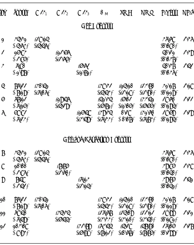
Table V presents the test results obtained using the iterated GMM procedure. The table contains four panels: Panel A contains test results obtained using data on all households, and consumption is deÞned as nondurables and services consumption. In panel B we repeat the same tests, again with nondurables and services consumption, but now only assetholders are included in the sample. Panels C and D repeat the analysis of panels A and B with consumption deÞned as total consumption, including durables. In each panel the top half presents results obtained using cohorts formed by grouping households in age cohorts, and the bottom part presents results obtained using cohorts formed by grouping households in age-education cohorts. Also, as mentioned in Section 2, each of the kernels is used with pricing factors constructed using individual data and also with pricing factors constructed using diﬀerent types of cohort data. Factors with a 1 subscript denote factors obtained using individual data. Factors with a 2 subscript denote cohort-based factors, where averaging is done on consumption. Factors with a 3 subscript denote cohort-based factors, where averaging is done on the consumption ratio.

In each panel in table V, we present results for estimation of (9) using the diﬀerent kernels for individual data and two sets of cohort data, leading to a total of 13 sets of results for every panel. Each row represents a set of estimation results and the J-statistic associated with the estimation exercise is listed in the last column.

Panel A presents results for nondurables and services consumption, with all households included in the sample. First consider the results associated with the pricing factors based on the individual consumption data in rows 1 and 7. The consumption growth factor is insigniÞcantly estimated. Also, the vcg1 factor is estimated with a negative sign.19

Interest-ingly though, whereas the CAPM kernel in row 13 is statistically rejected at the 5% level, this is not the case for the consumption-based kernels in rows 1 and 7.

The use of factors based on cohorts instead of individual data in rows 2, 3, 8 and 9 does not change these conclusions. In all cases the sign of the consumption dispersion is

19_{Positive correlation (conditional on the other factors) between the asset returns and the mcg factors} shows up with a negative sign, and negative correlation (conditional on the other factors) between the asset returns and the vcg factors shows up with a positive sign.

(23)

negative.20 Finally, consider the test results in rows 4, 5, 6, 10, 11 and 12. These results are obtained by combining two consumption-based factors with the market factor. In most cases point estimates and statistical signiÞcance for the consumption-based factors are quite similar to the corresponding cases in rows 1, 2, 3, 7, 8 and 9.

Panel B also presents results for nondurables and services consumption, but only house-holds that own assets are included in the sample. The results can be summarized very brießy. When using the individual data to construct the pricing factors in rows 1 and 7, we obtain a negative sign for average consumption growth and a negative sign for the variance of consumption growth. Compared to Panel A, statistical signiÞcance is higher. When using synthetic cohorts in rows 2, 3, 8 and 9, in some cases the factor vcg yields a positive sign. Finally, for the speciÞcations where the kernel depends on three factors in rows 4, 5, 6, 10, 11 and 12, the results are not very diﬀerent from those in Panel A. Summarizing, limiting the sample to assetholders does change the empirical results but test results are not necessarily consistent when constructing the cohorts in diﬀerent ways.

Panel C presents results obtained using all households, but the consumption measure used is total consumption instead of nondurables and services consumption. Inspection of Tables II through IV indicates that the cross-sectional distribution of the diﬀerent consumption measures is quite diﬀerent. However, when using individual consumption data in rows 1 and 7, results are again not encouraging. The factor mcg1 is estimated with the anticipated

negative sign and is statistically signiÞcant. Whereas the vcg1 factor is estimated with a

positive sign in some cases, the more relevant observation is that the estimate is statistically insigniÞcant. When using synthetic cohorts in rows 2, 3, 8 and 9, results are diﬀerent. In most cases we estimate the vcg2 and vcg3 factors with a statistically signiÞcant positive sign.

When the market factor is included as an additional factor, the consumption-based factors are still estimated signiÞcantly in most but not all cases. One observation that stands out is that the results obtained using the vcg3 factor are diﬀerent from the results obtained using

the vcg2 factor. This observation is similar to the Þndings in Panel B.

Given the results in Panels B and C, the results in Panel D are perhaps not totally surprising. This panel reports estimates obtained using data on total consumption, but only for households who hold assets. When using individual data in rows 1 and 7, estimates are not statistically signiÞcant. However, when constructing synthetic cohorts, the variance factors in rows 2, 3, 8 and 9 all yield statistically signiÞcant positive point estimates. Also, when adding the market factor to the two consumption-based factors in rows 5, 6, 11 and 12, empirical results for the consumption-based factors are not dramatically diﬀerent.

We perform a large number of robustness exercises that are not presented in the tables

20_{It is unclear how much emphasis should be put on the sign of the consumption dispersion factor. Our} primary concern is with the statistical and economic signiÞcance of consumption dispersion as a pricing factor, regardless of the sign. The sign on consumption dispersion reßects the evolution of the cross sectional distribution of consumption growth in recessions and expansions. To explain one particular empirical phenomenon, the equity premium puzzle, we need the sign to be positive.

(24)

because of space constraints. As mentioned above, we repeat the analysis after deseasonaliz-ing the data usdeseasonaliz-ing the census X11 method implemented in EVIEWS. Second, we correct the household consumption data for family size in two diﬀerent ways: by computing per capita data and by correcting for household size using a scale that is estimated from the data. Third, to address the problem that some cohorts contain few observations, we construct cohort pricing factors that are weighed by the size of the cohort. None of these adjustments impact signiÞcantly on the results.

Table VI further investigates the robustness of the results obtained in Table V, Panel D, using data on total consumption for asset holders only. We only report these results using one of the datasets to limit the number of tables. It must again be emphasized that the results for the three other datasets are possibly equally interesting from the perspective of pricing the cross-section of assets. We choose to focus on this dataset because the estimated sign of the consumption dispersion factor in Table V, Panel D, is also of interest for the related literature on the equity premium puzzle. Table VI clearly indicates the robustness of the results. Panel A presents the Þrst stage GMM estimates obtained by minimizing the HJ distance measure (13). We obtain positive estimates for the variance factors in all pricing kernels where we use factors based on cohort construction. It must be noted that the point estimates are not as signiÞcant as the ones in Table V, but this is to be expected because the Þrst stage GMM estimation is less efficient. The advantage of minimizing the HJ distance is that we can make comparisons of the HJ-distances obtained using the different kernels, because the same weighting matrix is used for different kernels. The performance of the consumption-based pricing factors is clearly impressive. The HJ-distance for the CAPM is 2.41 and serves as a benchmark. The HJ distances obtained when using factors constructed from individual consumption data in rows 1 and 7 are 2.33 in both cases. This is a lower HJ distance than for the CAPM, even though the variance factor is estimated insigniÞcantly. Most interestingly, the HJ distances are much lower when using factors based on cohorts. This is especially the case for the cohorts based on age in rows 2 and 3. When using a pricing kernel with two consumption-based factors and the market factor in rows 5, 6, 11 and 12, the HJ statistic drops even further.21 _{Panel B of Table VI provides two-step GMM}

estimates. Again, the results conÞrm those of Table V. The variance factors are estimated signiÞcantly positive whenever we use cohorts to construct pricing factors.

Table VII addresses an issue that was omitted from Tables V and VI because of space constraints. In Tables V and VI we always present consumption-based models with two factors. Given that this is an unconditional model and that we know that one-factor consumption-based models do not perform well in an unconditional setting, we therefore implicitly concluded that the extra second factor added explanatory power. Table VII

21_{The large HJ distances are due to the particular cross-section under investigation, not to the} inap-propriateness of the models. Because we use a challenging cross-section of portfolios sorted by size and book-to-market, it is to be expected that the HJ distance is high. The main focus is on the diﬀerences in HJ distance between diﬀerent factor pricing models.