Supertree methods for phylogenomics

HAL Id: tel-00842893

https://tel.archives-ouvertes.fr/tel-00842893

Submitted on 9 Jul 2013

HAL is a multi-disciplinary open access

archive for the deposit and dissemination of sci-entific research documents, whether they are pub-lished or not. The documents may come from teaching and research institutions in France or abroad, or from public or private research centers.

L’archive ouverte pluridisciplinaire HAL, est destinée au dépôt et à la diffusion de documents scientifiques de niveau recherche, publiés ou non, émanant des établissements d’enseignement et de recherche français ou étrangers, des laboratoires publics ou privés.

Celine Scornavacca

To cite this version:

Celine Scornavacca. Supertree methods for phylogenomics. Bioinformatics [q-bio.QM]. Université Montpellier II - Sciences et Techniques du Languedoc, 2009. English. �tel-00842893�

INFORMATION STRUCTURES SYSTEMES

P H D T H E S I S

to obtain the title of

PhD of Science

of the University of Montpellier II

Specialty : Computer Science

Defended by

Celine scornavacca

Supertree methods for

phylogenomics

Méthodes de superarbres pour la

phylogénomique

defended on December 8th, 2009

Jury :

Olivier Gascuel Directeur de recherche, CNRS Advisor Vincent Berry Professeur, UM2 Co-advisor Vincent Ranwez Maître de conférences, UM2 Co-advisor Marie-France Sagot Directeur de recherche, INRIA Referee Daniel Huson Professeur, Tübingen University Referee Simonetta Gribaldo Chargé de recherche, Institut Pasteur Examinator

All people say that acknowledgments are the last thing to write. So do I, but since my body is falling into pieces after having endured all these months of hard work, I hope to not forget someone.

First of all, I would like to thank Marie-France Sagot, Daniel Huson and Simon-etta Gribaldo for agreeing to be members of my thesis committee.

I would like to thank Olivier Gascuel for finding the time to read my thesis, although his time table is full until 2020, and to have improved it with his helpful comments.

What to say about VB & VR, i.e., Vincent Berry and Vincent Ranwez? It is difficult for me to imagine two better co-advisors. They accompanied me in the world of research, always encouraging me, inspiring me and leaving me free to make my choices. They are two excellent scientists and two nice and funny guys. A huge thank-you to my two-headed ogre (a citation for Warcraft fans only).

I wish to thank all the MAB team at the LIRMM for tolerating the high level of my voice in the hallways and for the interesting discussions.

A sincere thank-you to the members of the PPP team at the ISEM for show-ing me that evolution does not consist only in reconstructshow-ing supertrees, especially Emmanuel Douzery and Frédéric Delsuc.

I would like to thank the members of the LBBE team at the University of Lyon I, for welcoming me in France and for making the effort to understand the very bad French that I spoke at that time. A particular thank-you to Marie-France Sagot and Eric Tannier who have believed in me and have given me the possibility to start working in bioinformatics, to Vincent Daubin for his precious suggestions and to Sophie Abby and Simon Penel for their friendship.

Thanks also to all those people who have made my life in Montpellier pleasant. It is impossible to list them all, but a particular thank-you go to Rasta-Amine, for bringing fun and love in my life, Georgia Tsagkogeorga, for being a fantastic flat-mate and a really good friend, my moral support during this thesis. And Andrew Rodrigues, a true friend and a faithful climbing parter. I think that all people around me have to thank him to let me take it out on climbing walls rather than on people in the last part of the thesis.

Thank you to my friends that are far away, in Italy and all over the world. The Italian saying “Lontano dagli occhi, lontano dal cuore” does not work for me are they are still in my heart, especially Dada, Giacomone, Circy and Claudia.

A particular thank-you to Fabio Pardi for his help with the Shakespeare language (yes, some Italians can speak a good English!), to Juan Escobar and Samuel Blan-quart for answering to all my silly questions about evolution and to Julien Dutheil, who helped me a lot with the Bio++ libraries.

Thank also to Professor Gianpaolo Oriolo for introducing me to Eric Tannier and for giving me the possibility to do my Master stage at the University of Lyon I.

Finally I want to thank my family for their support. They taught me to love sciences and that hard work always pays. I really love you.

This thesis is dedicated to the memory of Roberta Dal Passo, a inspiring math-ematician and a true and frank person.

Introduction 1

1 Inferring phylogenies 5

1.1 From Aristotle to Darwin: an introduction . . . 5

1.2 Different types of biological data . . . 7

1.3 Parsimony methods. . . 9

1.4 Models of sequence evolution . . . 11

1.4.1 Nucleotide models . . . 11

1.4.2 Protein models . . . 14

1.4.3 Codon models. . . 14

1.5 Distance-based methods . . . 14

1.5.1 Estimation of evolutionary distances . . . 15

1.5.2 Least-squares methods . . . 16

1.5.3 Minimum-evolution methods . . . 17

1.6 Likelihood methods. . . 18

1.7 Bayesian methods. . . 19

1.8 Testing the reliability of inferred phylogenies. . . 21

2 Deeper insights on multiple data set analysis 23 2.1 Model inadequacy . . . 24

2.1.1 Compositional bias . . . 24

2.1.2 Heterotachy . . . 24

2.1.3 Rapidly evolving lineages . . . 25

2.2 Macro events . . . 25

2.2.1 Gene duplications and losses . . . 25

2.2.2 Horizontal gene transfers (HGT) . . . 27

2.2.3 Incomplete lineage sorting . . . 28

2.2.4 Interspecific recombination . . . 28

2.2.5 Interspecific hybridization . . . 29

2.3 Combining data. . . 29

2.3.1 Combining data through a supermatrix approach . . . 30

2.3.2 Combining data through a supertree approach. . . 32

2.3.3 The eternal dilemma: supermatrix or supertree? . . . 34

3 Methods for combining trees 37 3.1 Basic concepts . . . 39

3.1.1 Splits and clusters . . . 40

3.1.2 Quartets and triplets . . . 41

3.1.3 Interpretations of polytomies . . . 43

3.2.1 Consensus methods defined for both rooted and unrooted forests 44

3.2.2 Consensus methods defined only for rooted forests . . . 50

3.3 Supertree methods . . . 56

3.3.1 The OneTree supertree method and its variants . . . 57

3.3.2 Matrix Representation-based methods . . . 68

3.3.3 Median supertrees . . . 77

3.3.4 Other approaches to the supertree problem . . . 79

3.4 Which method to choose? . . . 82

4 Supertree methods from new principles 85 4.1 The PI and PC properties . . . 86

4.2 PhySIC . . . 90

4.2.1 The P hySICP C algorithm. . . 91

4.2.2 The P hySICP I algorithm . . . 93

4.2.3 The PhySIC algorithm . . . 94

4.3 PhySIC_IST . . . 95

4.3.1 The CIC criterion . . . 97

4.3.2 The PhySIC_IST algorithm . . . 99

4.3.3 Rooting the source trees . . . 106

4.3.4 The PhySIC_IST validation. . . 106

4.4 Combining supermatrix and supertree in Triticeea . . . 119

4.4.1 Triticeea: a problematic group . . . 119

4.4.2 Materials and Methods. . . 121

4.4.3 Results . . . 124

4.4.4 Discussion . . . 130

4.5 Conclusions . . . 135

5 Methods to include multi-labeled phylogenies in a supertree frame-work 137 5.1 Basic concepts and preliminary results . . . 139

5.1.1 Basic concepts . . . 139

5.1.2 Identifying observed duplication nodes in linear time . . . 140

5.2 Methods . . . 141

5.2.1 Isomorphic subtrees . . . 141

5.2.2 Auto-coherency of a MUL tree . . . 144

5.2.3 Computing a largest duplication-free subtree of a MUL tree . 150 5.2.4 Compatibility of single-labeled subtrees obtained from MUL trees . . . 152

5.3 Experiments . . . 154

5.3.1 Enlarging the amount of gene families to be used for species tree building . . . 155

5.3.2 Running times . . . 157

5.3.3 Improvement in supertree inference . . . 157

6 Conclusions and further research 163

7 Résumé en français 167

A Appendix to Chapter 4 179

A.1 Outline of main PhySIC subroutines . . . 179

A.2 Outline of main PhySIC_IST subroutines . . . 181

A.3 Supplementary materials of Section 4.4 . . . 185

It was three years and a half ago that I arrived in France. At the time, my work was focused on algorithms for Wi-Fi LAN. Yes, it was interesting but I needed to work on something more warm than computers. This is why I started working in the field of bioinformatics. Here I am, now, writing this manuscript after having spent several years in this marvelous world where mathematicians and computer scientists mix together with biologists and paleontologists to try to answer to one of the most fascinating questions ever asked: how all organisms on Earth descended from a common ancestor?

This thesis is about combining phylogenies. A phylogeny or phylogenetic tree consists in nodes connected by branches. Leaves, or terminal nodes, represent today organisms for which we can collect data. Internal nodes represent hypothetical ancestors since they cannot be directly observed. The aim of this thesis is to provide algorithms for the reconstruction of phylogenies and, ultimately, to estimate parts of the Tree of Life i.e., the phylogeny describing the relationships of all life on Earth in an evolutionary context.

In Chapter 1 we introduce the basic objects considered in this thesis, i.e., phylogenetic trees. Moreover, we briefly describe how phylogenies are inferred from biological data, to avoid the reader from thinking that they came “out of the blue” as a deus ex machina.

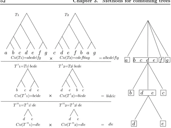
In Chapter2we review the biological phenomena that lead to produce different phylogenies from different data sets e.g., lateral gene transfers, gene duplications and losses. We also present two main approaches to combine different data sets to infer reliable phylogenies, with their pros and cons. The most straightforward approach to combine primary data issued from multiple sources is simply to concatenate them into a single data set called the supermatrix [Sanderson et al.,1998]. On the other hand, the supertree approach first involves inferring partially overlapping, source phylogenetic trees, that were inferred from primary data, and then assembling them into a larger, more comprehensive supertree [Bininda-Emonds,2004b]. In this thesis we focus on the latter approach. The supertree problem is a generalization of a simpler one, called the consensus problem, which consists in summarizing a set of trees that classify the same objects into one tree.

In Chapter 3 we thus present several consensus methods and we provide a review of most supertree methods currently available. We will see that some supertree methods are directly inspired by consensus methods, while others are based on new principles.

When using supertree construction in a divide-and-conquer approach in the at-tempt to reconstruct large portions of the Tree of Life, conservative supertree meth-ods have to be preferred in order to obtain reliable supertrees. In our opinion a

reliable supertree should display only information that is present in one or several input trees, or induced by their interaction. At the same time, it is desirable that the inferred tree contains as few contradictions as possible with the source trees.

In Chapter 4 we introduce two combinatorial properties we proposed that implement these ideas. Since no existing supertree method satisfies both these properties, we designed two supertree methods, PhySIC and PhySIC_IST [Ranwez

et al., 2007a; Scornavacca et al., 2008], which infer supertrees satisfying them.

A major difference between these two methods is that PhySIC_IST can propose non-plenary supertrees while PhySIC necessarily proposes a supertree that contains all taxa present in a least one source tree. Further we also designed a statistical preprocessing of the source trees to detect and correct artifactual positions of species. In this chapter we also present an example of application of PhySIC_IST to the complex problem of disentangling the phylogeny of Triticeae [Escobar et al.,

2009].

Gene trees are usually multi-labeled, i.e., a single species can label more than one leaf, since duplication events almost always resulted in the presence of several copies of the genes in the species genomes. Since no supertree method exists to combine multi-labeled trees, until now these trees are simply discarded in a supertree approach. In a phylogenomic framework, where the more data the better, this is not desirable.

In Chapter 5 we present a way to solve this problem, proposing several algorithms to extract the largest amount of speciation signal for orthologous sequences from multi-labeled trees, and put it under the form of single-labeled trees which can be handled by supertree methods [Scornavacca et al., 2009b]. An application to the hogenom database, a database of homologous genes from fully sequenced genomes, is presented.

In this work, the emphasis is on theoretical results, but real biological appli-cations are always kept in mind. The final product of my research tends to be algorithms for which user friendly implementations are freely available. Moreover, for each problem we encounter, biological case studies are presented to demonstrate the relevance of our approaches.

List of publications:

• Escobar, J., A. Cenci, C. Scornavacca, C. Guilhaumon, S. Santoni, E. Douzery, V. Ranwez, S. Glémin, and J. David. 2009. Combining supermatrix and supertree in Triticeea. Submitted to Systematic Biology.

• Ranwez, V., V. Berry, A. Criscuolo, P. Fabre, S. Guillemot, C. Scornavacca, and E. Douzery. 2007. PhySIC: a veto supertree method with desirable properties. Systematic Biology 56:798–817.

PhySIC_IST: cleaning source trees to infer more informative su-pertrees. BMC Bioinformatics

• Scornavacca, C., V. Berry, and V. Ranwez. 2009b. From gene trees to species trees through a supertree approach. Pages 702–714 in LATA ’09: Pro-ceedings of the 3rd International Conference on Language and Automata The-ory and Applications, volume 5457 of Lecture Notes in Computer Science, Springer- Verlag, Berlin, Heidelberg. 9:413.

• Scornavacca, C., V. Berry, and V. Ranwez. 2009a. Building species trees from larger parts of phylogenomic databases. Submitted to Information and Computation.

Inferring phylogenies

Contents

1.1 From Aristotle to Darwin: an introduction . . . 5

1.2 Different types of biological data . . . 7

1.3 Parsimony methods . . . 9

1.4 Models of sequence evolution . . . 11

1.4.1 Nucleotide models . . . 11

1.4.2 Protein models . . . 14

1.4.3 Codon models . . . 14

1.5 Distance-based methods . . . 14

1.5.1 Estimation of evolutionary distances . . . 15

1.5.2 Least-squares methods . . . 16

1.5.3 Minimum-evolution methods . . . 17

1.6 Likelihood methods . . . 18

1.7 Bayesian methods . . . 19

1.8 Testing the reliability of inferred phylogenies . . . 21

Men are curious. Scientists even more. A question that fascinates an increasing number of scientists, especially since the last decades, is to understand how all organisms on Earth descended from a common ancestor. Phylogenetics is the sub-field of evolutionary biology that studies evolutionary relationships among species through molecular and morphological data.

In this chapter we present how phylogenetics arose as a science and a review of the field.

1.1

From Aristotle to Darwin: an introduction

Since Aristotle, naturalists have always tried to classify the abundance of creatures that populate the Earth. Aristotle believed that creatures were arranged in a graded scale of perfection rising from plants up to man that he called the scala naturae. Aristotle’s classification of living, even if now completely outdated, contains some truth. For example, he was the first to divide beings in vertebrates and invertebrates (called animals with and without blood in his work). During the Middle-Age and Renaissance almost no progress was done.

The quest of this natural order was the major goal of naturalists of the eigh-teenth century. Linneaus, maybe the most famous of the systematists, believed in an underlying order in nature that needs to be discovered and expressed as a hierar-chy. At his time, classifications of living things were built using as discriminant the phenotype, i.e., any observable characteristics of organisms. Linneaus thought that a reliable discriminant was a character good for ordering as many beings as possi-ble. This method sometimes led Linneaus to classifications that now we consider erroneous. A significant improvement to Linneaus’ method was the proposal of the natural classification by Antoine Laurent de Jussieu, based on the use of multiple characters to define groups. No matter the way the groups were formed, in those days all classifications were proposed in the framework of fixism, a theory stating that life on Earth has always been composed of the species we have today and that species never change.

The first naturalist to evoke the possibility that species can evolve was Leclerc de Buffon. He pointed out an evident continuity among individuals of the same species and a less evident, but present, continuity among species. For Buffon the classification was nothing more than an artifact that had to be replaced by the concept of descent.

Jean-Baptiste Lamarck was the first to propose an evolutionary theory. In his oeuvre Philosophie zoologique (1809) he introduced the concept of the general dis-tribution, i.e., an order produced by the walk of nature in living creatures that are seen as being in perpetual evolution. Lamarck was also a fervent opposer of the concept of classification that, for him, «has nothing natural». For Lamarck, the aim of understanding the general distribution was not to be able to classify living creatures but to understand the order that nature followed to produce them. The concept of spontaneous generation of life from inanimate matter prevents Lamarck from proposing a genealogy of living. This is, together with the notion of inheritance of acquired characters, one of the weakest points of his theory.

In The Origins of Species (1859), Charles Darwin introduced his theory accord-ing to which populations evolve over the course of generations through a process of natural selection and the variability of life arose through a branching pattern of evolution and common descent. He illustrated his theory using a tree where ac-tual species are linked two by two up to a common ancestor species. For Darwin, species could undergo several mutations but the history of life was unique. Others before Darwin used trees to illustrate species classifications in light of fixism (e.g., Augustin Augier) or descent of some species from others (e.g., Charles-Hélion de Barbançois). The originality of Darwin’s tree is the coexistence, in the same figure, of the concepts of time and descent: the bifurcations in the tree follow one another over time. It is interesting to note that, unlike Lamarck, Darwin was not a detractor of the concept of classification. For him, once that genealogy of species was found, it would lead to the “natural” classification of living creatures.

It was Ernst Haeckel in 1866 that used for the first time the term phylogeny to designate the history of organismal lineages as they change through time. At his

time, phylogenies were built using morphological traits, ontogeny1

and fossils. With the discovery of DNA by Watson and Crick in 1953 and the design of sequencing techniques, a new kind of information became available: molecular data. Thanks to the huge amount of information available since 10-20 years, phylogenetics entered in its golden age. At that time, some of the problems that are treated in this thesis arose.

Phylogenetics aims at clarifying the evolutionary relationships that exist among different species, represented through phylogenetic trees or phylogenies. A phylogeny2

consists in nodes connected by branches (see Figure1.1for an example). Terminal nodes are called leaves or taxa and represent today organisms for which we can collect data. Internal nodes represent hypothetical ancestors since they cannot be directly observed. In rooted phylogenetic trees (see Figure 1.1(i)), each internal node represents the most recent common ancestor of its descendants and the only node with no ancestor is called the root of the tree. Nodes and branches can have several kinds of information associated with them, such as time or amount of evolution estimates.

1.2

Different types of biological data

Phylogeny reconstruction methods are used to analyze either morphological (struc-tural aspects of organisms such as bone structure, organs, etc.) or molecular (genetic information such as nucleotides, amino acids, codons, SINE or LINE etc.) data. We can consider these data as sequences of characters that can take several states ({0,1} for the presence/absence of a morphological trait, {A,C,G,T} for nucleotidic sites etc.).

To properly reconstruct phylogenies, it is important to be able to determine which characteristics are similar because they were inherited from a common ances-tor (homology) and which are similar as a result of separate convergent evolution (homoplasy). For morphological data, we might consider similar looking features to be homologous when they are not and the similarity is a result of convergent evolution (e.g., the wings of bats and birds). Because the homology among proteins and DNA is often concluded on the basis of sequence similarity, such problems can also arise with molecular data (for example because of gene duplication events3

). Moreover, if we want to use molecular data to reconstruct phylogenies, we have to face another problem. For morphological traits, we can only have that the state for a character of a species changes or not in its descendants. In molecular sequences, we can have substitutions (modifications of the site state) as well, but insertions and deletions of some sites are also possible. The result is that the same

1

Ontogeny is the branch of biology that deals with the development of an individual organism from the fertilized egg to its mature form.

2

For a formal definition of phylogeny see Chapter3. 3

(i

)

(ii

)

Figure 1.1: Phylogenetic trees for the Glioma tumor suppressor candidate region gene 1 protein marker (ENSG00000063169), obtained with a max-imum likelihood (ML) analysis [Ranwez et al.,2007b] - where branch lengths represent amounts of evolution between species. Note that in the phylogenetic tree in (i) nodes are connected to other nodes by a horizontal and then a vertical line but only vertical branch lengths represent amounts of evolution. The only difference between these two trees is that the one in (i) is rooted, whereas the one in (ii) is not. In a rooted tree, the root corresponds to the most recent common ancestor of the leaves. This information and therefore the direction of evolution (from the root to the leaves) are lost in an unrooted tree.

molecular marker in different species has different lengths. When this happens, we need to align the sequences correctly to be sure that we are really comparing the same characters in all species. A variety of algorithms have been designed to solve the sequence alignment problem, including dynamic programming methods, heuristic algorithms and probabilistic methods. That is why in the following sections we will consider only aligned sets of sequences of same length.

To reconstruct phylogenies two kinds of methods are available:

• character-based methods, which retrieve similarities comparing the states taken by species at different characters; character-based methods can be fur-ther divided into:

– parsimony methods – likelihood methods – bayesian methods

• distance-based methods, which use pairwise distances to quantify the amount of evolution separating species.

1.3

Parsimony methods

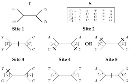
The main hypothesis of these methods is that evolution is parsimonious and the most plausible phylogenies are that requiring the fewest evolutionary changes to explain data. Parsimony methods are based on discrete characters. Input data consist in a set S of n character sequences (one per studied species) s1, ..., sn of length m.

The two most widespread variants of parsimony are the Fitch parsimony, where the cost of substituting a state with another is equal to 1 for all states [Fitch,1971], and Sankoff parsimony, where a substitution cost Cx→y is associated to each pair of

states x, y, with x�= y [Sankoff and Rousseau, 1975]. Fitch parsimony is a special case of the Sankoff parsimony but the algorithm that Fitch proposed for it is not a special case of Sankoff algorithm [Felsenstein, 2004].

Other types of parsimony have been proposed e.g., Dollo parsimony [Farris,1977;

Le Quesne,1974] and Camin-Sokal parsimony [Camin and Sokal,1974].

In a parsimony approach each character can be analyzed independently from the others. It follows that, given a phylogeny T , once the parsimony score P(cj|T ) is

calculated for each character cj, the parsimony score of the set S of all sequences is

given by the (weighted) sum of the parsimony score of each character: P (S|T ) =

m

�

j=1

wjP (cj|T ) (1.1)

where wj is the weight of character cj. Assuming that internal sequences are known

(see figure 1.2) one can easily determine the number of substitutions necessary to explain different states for cj at the two extremities of a branch e. Denoting this

value by P (cj|e), P (cj|T ) is simply the sum of P (cj|e) over all branches e of T ,

weighted by the substitution costs.

TAGTA TAGTA CAGTG TATTA TCGTA S! S" CAGTG CCGTG S# S$

Figure 1.2: One of the most parsimonious phylogenies for the set of se-quences S ={S1, S2, S3, S4}. - The five required substitutions are indicated by small horizontal lines.

Since only terminal sequences are known, we need to find the combination of internal sequences that minimizes P (cj|T ) (see Figure 1.3). This problem is not as

• the number of possible states for a character is limited; • each character can be analyze independently;

• the choice of the root does not change the parsimony value of a tree, in the usual case where Cx→y = Cy→x holds for each pair of states x, y.

An O(nm) algorithm to calculate P (S|T ) was proposed by Fitch [1971]. On the contrary, finding the tree T that gives the minimum value of P (S|T ) is an NP-hard problem [Day et al., 1986] for which several heuristic methods were proposed

[Felsenstein, 2005;Goloboff et al.,2008; Swofford,2003].

T G G G G G T T T T T T A A G G A G

Site 3 Site 4 Site 5

A C A C C C T C T C T C Site 1 Site 2 A C A C A A OR S! S" S# S$ T S! = S" = S# = S$ = T T C C A C A C T G G G T T T T A A G G S

Figure 1.3: Most parsimonious reconstructions per sites for the set of se-quences S given the phylogeny T - Two equally parsimonious reconstructions are possible for site 2. Deduced internal characters are shown between square brackets. The main drawback of parsimony methods is that they are not consistent [

Caven-der, 1978; Felsenstein, 1978]. A method is said to be consistent if the probability

to obtain the correct tree converges to one as more and more data are analyzed. For example, parsimony methods are not robust to long branch attractions i.e., when rapidly evolving species that had a separated evolution are inferred to be closely related, regardless of their true evolutionary relationships [e.g., Felsenstein,

1978, see Section2.1.3]. Indeed, when molecular sequences from two species evolve rapidly, the probability that the same nucleotide appears in both two sequences at the same site increases. When this happens, the most parsimonious scenario is a wrong one, where the two species evolved from a common ancestor. As a matter of fact, rapid evolving species accumulate numerous mutations on a single character and contradict the very foundations of the parsimony approach. For a review of other objections to parsimony methods seeSober [1998].

1.4

Models of sequence evolution

The main limitation of parsimony methods is to try to reconstruct phylogenies without making assumptions on the underlying evolutionary process that species undergo.

At the end of the sixties, the first model of DNA evolution was proposed [Jukes

and Cantor, 1969]. The aim of models describing the evolution of sequences is to

provide a formal framework to estimate the real number of mutations that a sequence has undergone rather than simply assuming that this number is minimal. This framework has allowed to develop statistically consistent reconstruction methods such that, if the underlying evolutionary model is correct, the method asymptotically converges to the real phylogeny. This section presents a short review of the best known models of nucleotide sequence evolution and evokes protein sequences and codon models. This will be useful in Sections from1.5to1.7.

1.4.1

Nucleotide models

Most nucleotide substitution models share some common hypotheses:

• sequences evolve exclusively through nucleotide substitutions. Nucleotide in-sertions and deletions are not taken into account;

• substitution processes are independent and identical among sites: substitu-tions affecting one site do not depend either on substitusubstitu-tions affecting other sites or on the position of the site in the sequence. This implies that knowing the substitution process of sites means knowing that of the sequences; • substitution process is a first-order Markov model. Having a memory of size

1, the evolution of sequences depends only on the actual state of sequences and not on its previous states;

• substitution process is homogeneous, i.e., it is the same for all branches of the phylogeny and independent among branches;

• substitution process is stationary, i.e., the probability to observe a state x (denoted by πx) does not depend on the position of the observation date;

• the substitution probability during an infinitesimal time interval dt is propor-tional to dt.

• there is at most one substitution per infinitesimal time interval dt.

Nucleotides are modeled as discrete characters that can vary in the set of bases {A, C, G, T }. Nucleotide models are characterized by a 4 × 4 rate matrix Q where Qxy is the rate at which base x goes to base y. The general expression of Q is the

Q =     λA QAC QAG QAT QCA λC QCG QCT QGA QGC λG QGT QT A QT C QT G λT     (1.2)

where λx =−�_x�=yQxy. The probability matrix is obtained from the rate matrix

by computing the system P (t) = eQt_{. The general expression of P (t) is the following:}

P (t) =     ¯ λA(t) PAC(t) PAG(t) PAT(t) PCA(t) λ¯C(t) PCG(t) PCT(t) PGA(t) PGC(t) ¯λG(t) PGT(t) PT A(t) PT C(t) PT G(t) ¯λT(t)     (1.3)

where Pxy(t) is the probability that a base x changes into a base y in a time interval

t and ¯λx(t) = 1−�x�=yPxy(t).

Time Reversibility

A stationary Markov process is time reversible if (in the steady state) the amount of change from state x to state y is equal to the amount of change from y to x. Almost all DNA evolution models assume time reversibility i.e., that ∀x, y ∈ {A, C, G, T } we have Mxyπx= Myxπy.

General Time Reversibility (GTR) model

Under this assumption, the general expression of Q in1.2becomes:

QGT R =     λA πCRAC πGRAG πTRAT πARAC λC πGRCG πTRCT πARAG πCRCG λG πTRGT πARAT πCRCT πGRGT λT     (1.4)

where the term Rxy is equal to Mxy/πy.

The GTR substitution model [Tavaré,1986;Yang,1994] requires 6 substitution rate parameters, as well as 4 base frequency parameters. Since� πx= 1 there are

only 3 free frequency parameters. Moreover, if rate parameters are considered as relative rate parameters, one rate can be fixed to 1 (e.g., RGT). It follows that the

number of free parameters of the GTR model is equal to 8. All models in table

1.4.1 are particular cases of the GTR model. Some models assume Equal Base Frequencies (EBF=y) i.e., πx = 0.25 ∀x ∈ {A, C, G, T }. All other models assume

that πC�= πG�= πA�= πT, except the T92 model that hypothesizes πC= πG= π/2

and πA= πT = (1−π)/2. Models with a Number of Different Types of Substitutions

(NDTS) equal to 1 suppose that Rxy= α,∀x, y ∈ {A, C, G, T }, x �= y. Models with

NDTS_{= 2 distinguish between transitions (A <-> G, i.e., changes from purine to} purine, or C <-> T, i.e., changes from pyrimidine to pyrimidine) and transversions (from purine to pyrimidine or vice versa). Models with NDTS = 3 distinguish

between the two different types of transition, i.e., RAG�= RCT while transversions

are all assumed to occur at the same rate. Several other special cases of the GTR

Model NDTS EBF TNP

JC69 [Jukes and Cantor,1969] 1 y 0

F81 [Felsenstein,1981] 1 n 3

K80 or K2P [Kimura, 1980] 2 y 1

HKY85 [Hasegawa et al.,1985b] 2 n 4

F84 [Kishino and Hasegawa, 1989]

[Felsenstein and Churchill,1996] 2 n 4

T92 [Tamura,1992] 2 n 2

K3ST [Kimura, 1981] 3 y 2

TN93 [Tamura and Nei, 1993] 3 n 5

SYM [Zharkikh and Li,1995] 6 y 5

Table 1.1: Nucleotide models that are special cases of the GTR model-NDTS_{is the Number of Different Types of Substitutions distinguished by the model,} EBF_{specifies whether the model assumes Equal Base Frequencies and TNP is its} Total Number of free Parameters.

model have been described and named. More complex models

The models described above all assume that each position is evolving independently and identically. Site to site rate variation has also been modeled, mostly by a gamma distribution among sites [Yang, 1993, 1996a] and the presence of a proportion of invariable sites in the data set [Hasegawa et al., 1987]. The gamma distribution, introduced in molecular evolution byUzzell and Corbin[1971] and developed byJin

and Nei[1990] andYang [1993], has several advantages: it is analytically tractable,

varies from 0 to∞ and has a single parameter to control both the distribution shape and its mean and variance.

Galtier and Gouy[1998] proposed models for which the substitution process is

non-homogeneous, i.e., model parameters are not the same for all branches of the phylogeny and can vary at the nodes of the tree. Galtier[2001] proposed heterotac-hous models of sequence evolution for which rates of evolution can vary among sites. Both the proportion of sites undergoing rate changes and the rate of rate change are free variables. Note that Galtier’s 2001 model provides an alternative to the gamma distribution of rates across sites.

The CAT mixture model [Lartillot and Philippe, 2004] accounts for across-site heterogeneities of the substitutional processes. The total number of classes of the underlying mixture is not specified a priori, but is a free variable of the model.

The BP model [Blanquart and Lartillot,2006] permits model parameters to vary along the phylogeny, changing not only at every node as inGaltier and Gouy[1998],

but also along branches.

The CAT+BP model [Blanquart and Lartillot,2008] combines the CAT and BP models.

The latter three models are very complex and computationally demanding and have only been implemented into Bayesian frameworks (see section 1.7).

Several other methods have been recently proposed (for a review see Galtier

et al. [2005]).

Adding parameters will almost always improve fit to data, but also leads to a larger estimation error. To discourage overfitting, statistical tests that attempt to find the model that best explains the data with a minimum of free parameters have been proposed (e.g., the AIC [Akaike,1974] and the BIC [Schwarz,1978]).

1.4.2

Protein models

The first amino acid models have been proposed at the end of the 1970s. The main advantage in favor of using amino acid information is the fact that DNA undergoes much more back substitutions, making it harder to accurately recover tree evolu-tionary histories, especially those with long evoluevolu-tionary distances. Since in nature there exist 20 amino acids, a GTR-like model for proteins would require 208 param-eters and would be overparameterized for most data sets. That is why models of protein evolution are often based on empirical matrices that are obtained averaging the observed changes and amino acid frequencies between numerous proteins. The resulting matrices state the relative rates of replacement from one amino acid to another. The most commonly used protein models are PAM [Dayhoff et al., 1978], JTT [Jones et al., 1992], Blosum62 [Henikoff and Henikoff, 1992], WAG [Whelan

and Goldman,2001] and LG [Le and Gascuel,2008] matrices.

Note that the CAT and the BP models afore-described can also be used to model protein evolution.

1.4.3

Codon models

Lately, models of codon evolution have been proposed [Goldman and Yang, 1994]. They are used mainly to infer the selection forces acting on a protein that can be hidden by the fact that most amino acids are encoded by more than one codon4

. This degeneracy of the genetic code allows substitutions to occur in the DNA sequence that do not result in a change in the corresponding amino acid sequence. For a review of existing codon models see Delport et al.[2009].

1.5

Distance-based methods

Distance-based methods use pairwise evolutionary distances to reconstruct phylo-genies. But how do we calculate those distances?

4

1.5.1

Estimation of evolutionary distances

The evolutionary distance Dsz between two sequences s and z is defined as the

average number of substitution events per site that have occurred since s and z have diverged. A rough estimate for Dszis given by fsz, defined as the proportion of sites

that have different states in s and z. The observed value fsz is an underestimate of

Dsz since it cannot take into account such events as multiple, parallel, convergent,

coincidental and back substitutions. Better estimations of Dsz can be found if we

use a substitution model such as those described in the previous section since this would allow to take into account multiple substitutions for a single site. Let suppose we choose JC69 as model and denote by α the unique substitution rate. In this case, computing the system P (t) = eQt _{we obtain:}

Pxy(t) =    1 4(1− e−4αt) if x�= y 1 4(1 + 3e−4αt) otherwise (1.5)

Suppose that a time t elapsed since the divergence of the two sequences. Then the two sequences are separated by a time 2t and we can easily calculate the probability for a site to have different states in s and z, denoted by psz(t):

psz(t) = 3 4(1− e −8αt_{) (1.6)} It follows that: αt =−1 8ln(1− 4 3psz(t)) (1.7)

From the definition of α, the average number of substitution events per site that occurred since s and z diverged, i.e., Dsz, can be estimated by 2t×3α, because each

site changes its state with a probability 3α per time unit. This implies that: Dsz=−3

4ln(1− 4

3psz(t)) (1.8)

Since psz(t) = E(fsz), we can use fsz to estimate psz(t). Then we obtain:

ˆ Dsz=− 3 4ln(1− 4 3fsz) (1.9)

which is a better estimation of Dsz than fsz.

For other simple models, analytical formulae for the estimation of Dsz are

available. If the model is too complex a likelihood optimization (see Section1.6) is used to estimate ˆD. Other kinds of distances have been proposed e.g., the LogDet distance [Barry and Hartigan, 1987; Steel, 1994]. For a review of evolutionary distances seeZharkikh [1994].

Phylogeny-reconstruction distance methods are applied to dissimilarity matrices ˆ

D obtained from sequence matrices (see above). Ideally, the aim of these methods is to find the phylogeny T such that the length of the path between species s and z

in T , also called patristic distance of s and z, is equal to ˆDsz. If there exists a tree

whose patristic distances are ˆD, ˆD is said to be a tree distance. Since we do not have the real distances but only an estimation of them, usually no such tree exists. A result obtained independently by several authors [among othersBuneman,1971] states the properties that a distance matrix ˆD has to satisfy to be a tree distance: Proposition 1.5.1 ˆDsz is a tree distance (also called additive) if and only if it

verifies the following three conditions:

• ˆDsz �0 between two different species, and is zero if and only if s = z,

• it is symmetric, i.e., ˆDsz = ˆDzs,

• for all quadruplets of species (s,z,t,u), ˆDsz+ ˆDtu�max{ ˆDst+ ˆDzu, ˆDsu+ ˆDzt}.

The third condition is often called the four point condition. Since dissimilarity matrices obtained as explained above hardly ever verify the four point condition, the goal of distance methods is to find the phylogeny T whose patristic distances are as close as possible to ˆD. The way of defining what a “as close as possible” means varies to one distance method to another. In the next sections we present the most used distance methods.

1.5.2

Least-squares methods

Least-squares methods (LS) aim at adjusting the given distance matrix ˆD to obtain a tree distance ˇD that minimizes a measure of discrepancy, defined as follows:

Q =�

s<z

wsz( ˆDsz− ˇDsz)2 (1.10)

where wsz are weights that differ among least-squares methods and are used to

account for the uncertainty on the value of ˆDsz. If wsz = 1, formula1.10corresponds

to the ordinary least-squares criterion [Cavalli-Sforza and Edwards,1967]. Otherwise we have a weighted least-squares criterion. Commonly used weights are 1/ ˆDsz[Beyer

et al.,1974] and 1/( ˆDsz)2 [Fitch and Margoliash,1967].

For a given phylogeny T , the tree distance minimizing any least-squares criterion can be found in polynomial time. This approach was first presented byCavalli-Sforza

and Edwards [1967] and improved by Gascuel [1997b] and Bryant and Waddell

[1998]. On the contrary, finding the best phylogeny minimizing Q is an NP-hard problem [Day,1987,1996] for which several heuristic methods have been proposed. Some variations of the least-squares criterion, called the generalized least-squares criterion, have been proposed to take into account the natural correlations between distances [Bulmer,1991; Susko,2003].

1.5.3

Minimum-evolution methods

The minimum evolution method (ME) aims at minimizing the total length of the reconstructed tree T , i.e.,

Q =�

e∈T

l(e) (1.11)

where l(e) is the length of the branch e and branch lengths, which represent quanti-ties of evolution, are computed using a least-squares method. In a minimum evolu-tion approach, the most plausible phylogeny is that demanding the minimum quan-tity of evolution. This approach has been first proposed by Kidd and

Sgaramella-Zonta[1971] and developed byRzhetsky and Nei[1992]. It has been proved [Denis

and Gascuel, 2003; Rzhetsky and Nei, 1993] that if the estimation of ˆDsz tends to

Dsz and branch lengths are estimated with an ordinary least-squares criterion, then

the method converges to the correct phylogeny i.e., it is consistent. On the contrary,

Gascuel et al.[2001] have proved that some weighted and generalized least-squares

methods, if used to estimate branch lengths, lead to inconsistent versions of the min-imum evolution method. Since in the minmin-imum evolution approach branch lengths are computed using a least-squares method, methods that improve the complex-ity and running time of the latter methods [e.g., Bryant and Waddell, 1998], also speed up the former. Improved search methods have also been proposed [Desper

and Gascuel,2002; Kumar, 1996].

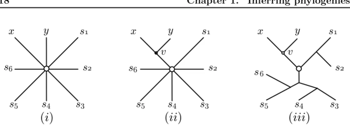
Clustering methods for the minimum evolution approach have been proposed. They first construct a star tree connecting one central node to leaf nodes representing all species for which we have distances (Figure1.4(i)). At each step a pair of nodes x, y to cluster is chosen using the information contained in the distance matrix ˆD. The two nodes are then connected to a new node v that is in turn connected to the central node (Figure1.4(ii)). The two rows and columns corresponding to x and y are removed from the matrix ˆD while an extra row and an extra column are added to ˆD for the new node v. On the whole, the dimension of ˆD is decreased by 1. Then the distances ˆDiv between all nodes i in the matrix and v are computed. After

n− 2 steps a completely resolved phylogeny is obtained (Figure 1.4(iii)), where n is the number of species. Clustering methods vary in the way they choose nodes to cluster and compute the new distances ˆDiv. The most widely used are NJ [Saitou

and Nei, 1987], UNJ [Gascuel, 1997b], BIONJ [Gascuel, 1997a] and WEIGHBOR

[Bruno et al.,2000].

A heuristic method for the ME that is not clustering-based is FASTME [Desper

and Gascuel, 2002] that aims at minimizing the balanced minimum evolution

cri-terion introduced by Pauplin [2000]. Also NJ is a heuristic for the same criterion as proved by Gascuel and Steel [2006], while UNJ is a heuristic to minimize the ordinary least-squares version of ME.

s! s! s# s" s$ x y

(iii)

s% v x y s$ s" s#

(ii)

s% v s" s# s!

(i)

x y s$ s%

s& s& _s&

Figure 1.4: The clustering process to build a phylogenetic tree - (i) the initial situation. (ii) the first clustering groups x and y. (c) the final situation.

1.6

Likelihood methods

Likelihood methods were first introduced in phylogeny by Edwards and

Cavalli-Sforza[1964] to deal with gene frequency data. The first applications to molecular

sequences was proposed by Neyman [1971] and improved by Kashyap and Subas

[1974] andFelsenstein[1981].

In this section and in the following one, we denote as θ the vector of all the parameters of an evolutionary model, where here an evolutionary model is the com-bination of a substitution model M (see Section 1.4), a topology and its branch lengths.

Given a sequence alignment S of n character sequences (one per studied species) of length m and a vector of parameters of an evolutionary model θ, the likelihood of θ, denoted by P(S|θ), is defined as the probability to observe the data set S, given θ. The likelihood can be viewed as a function of θ.

The hypothesis of the independence of the evolution of each site, already evoked in Section 1.4.1, implies that

P(S|θ) =

m

�

j=1

P(cj|θ) (1.12)

This simplifies a lot the calculation of the likelihood. When the vector θ is given, the topology of T is known. In such a case, to compute the likelihood of a site cj, we

asso-ciate at each node u∈ T a likelihood vector Lcj,u = (Lcj,u,A, Lcj,u,T, Lcj,u,G, Lcj,u,C),

where Lcj,u,x is the probability of observing the state x at the node u, with

x ∈ {A, T, G, C}. The reversibility hypothesis, assumed by most models of se-quence evolution, implies that the likelihood of T does not depend on the position of the root [Felsenstein, 1981, the “pulley principle”]. We can then compute the likelihood of an unrooted phylogeny rooting it on whatever branch or node. Once the tree is rooted, the algorithm starts initializing the likelihood vectors associated to each leaf of T in the following way: Lcj,u,x = 1 if the leaf u has state x at the

site cj, otherwise Lcj,u,x = 0. If the state of site cj is unknown, then Lcj,u,x = 1

a bottom-up tree traversal i.e., a node cannot be treated before all its sons have been. For each internal node u, its likelihood vector is computed from the likelihood vectors of its sons l(u) and r(u) as follows:

Lcj,u,x= � � y∈{A,T,G,C} Pxy(bu,luu)) · Lcj,l(u),y � · � � y∈{A,T,G,C} Pxy(bu,r(u)) · Lcj,r(u),y � (1.13) where bu,l(u), resp bu,r(u), is the length of the branch (u,l(u)), resp (u, r(u)). The

likelihood P(cj|θ) for the site cj is defined as the product:

�

x∈{A,T,G,C}

πxLcj,r,x (1.14)

where r is the root node of T and πx is the equilibrium probability of the base x

under the model M . Using this dynamic programming technique [Felsenstein,1981], the likelihood of T can be computed in O(nm), where n is the number of sequences and m the number of characters of the alignment. Unfortunately, when trying to reconstruct a phylogeny from sequences, θ is unknown. This means that, to find the phylogeny with maximum likelihood, we also need to consider all combinations of its parameters. This is the main limit of this approach, but for simple evolutionary models, when the likelihood of a tree can rapidly be computed, efficient heuristics have been developed. These methods are considered as being among those inferring the most reliable phylogenies.

Heuristic methods for the maximum likelihood approach have been implemented in several programs, e.g., PAUP* [Swofford,2003], PHYML [Guindon and Gascuel,

2003], IQPNNI [Vinh and Von Haeseler, 2004], RAxML [Stamatakis, 2006] and GARLI [Zwickl,2006]. The latter uses a stochastic, genetic algorithm-like approach instead of deterministic hill climbing.

For complex methods for which analytical solutions cannot be found even when θ is known, an ML approach is not tractable. That is why a bayesian approach to phylogeny reconstruction has been proposed.

1.7

Bayesian methods

Bayesian methods to infer phylogenies are closely related to likelihood methods. Bayesian inference of phylogeny is based on a quantity called the posterior probabil-ity of a parameter vector θ of an evolutionary model, given a sequence alignment S, denoted by P(θ|S). Bayes’ theorem allows to turn a prior distribution of θ, denoted by P(θ) into its posterior distribution:

P(θ|S) = P(θ)P(S|θ)_P(S) (1.15)

where P(S|θ) is the likelihood of the sequence alignment S given the parameter vector θ. The posterior probability of θ can be interpreted as the probability that

the parameter vector θ is the correct one. In order not to influence the result with personal opinions, a flat prior can be assigned. It is also possible to assign vague priors [Huelsenbeck et al., 2002b]. Note that the ML approach is a particular case of the bayesian approach, for which flat prior are chosen [Kuhner et al.,1995]. The denominator in1.15involves a summation over all trees and, for each tree an inte-gration over all possible branch lengths and parameters of the substitution model. This computation is often analytically impossible, but numerical methods can be used to efficiently approximate the distribution of posterior probability. The most used are Markov Chain Monte Carlo (MCMC) methods [e.g., Gilks et al., 1995] that permit to wander randomly through the posterior distribution over parameter and tree space. Once this random walk reaches equilibrium, samples of parameter vectors are collected and will be used to approximate their posterior probability dis-tribution. For phylogeny inference, the MCMC algorithm is based on the Metropolis algorithm [Metropolis et al., 1953] and consists of the following steps:

1. start with a random vector of parameters θi;

2. select a new vector θj by modifying θi in some way;

3. compute the acceptance ratio R = P(θj|S)

P(θi|S)

= P(θj)P(S|θj) P(θi)P(S|θi)

; 4. accept θj with a probability ρ=max(R, 1);

5. every k generations, save the current tree and all parameters; 6. return to step 2.

Note that denominator in1.15disappears in the computation of R. This algorithm has no termination. It is up to the user to stop it after a number of generations considered sufficient. This is one of the limits of this approach. Note also that this algorithm is a Markov chain of order one since θj depends only on θi. We call

the vector of parameters θi the “state θi”. To reach the equilibrium distribution,

the Markov chain must be aperiodic (no cycles should be present in the Markov chain), irreducible (every state must be accessible from any other state), and the probability of proposing θj if the current state is θi has to be the same as that of

proposing θi if we are in θj, denoted respectively by P(θj|θi) and P(θi|θj). If this

is not true, a variant of Metropolis algorithm, the Metropolis-Hasting algorithm

[Hastings, 1970] has to be used. Hasting’s algorithm differs from the Metropolis’

one in the computation of the acceptance ratio, which equals R· P(θj|θi)

P(θi|θj). When

the Markov chain has the required properties to reach the equilibrium and is run long enough, the time the chain spends in a state θi is proportional to its posterior

probability [Metropolis et al., 1953].

If the target distribution has multiple local peaks, separated by low valleys, the Markov chain may have difficulty in moving from one peak to another. As a result,

the chain may get stuck on one peak and the resulting samples will not approximate the posterior probability correctly. Metropolis Coupled MCMC (called also MC3_{), a}

variant of MCMC, allows multiple peaks in the landscape of trees to be more readily explored. This technique consists roughly in running k MCMC chains with different stationary distributions. One chain is called the cold chain and only its information is recorded. Periodically, states between chains may be swapped.

Bayesian methods vary in the way they set prior distributions for parameters, obtain the state θj from θi and summarize the information of the obtained samples

(step 5). Several bayesian approaches for phylogeny reconstruction have been re-cently proposed [e.g.,Huelsenbeck et al., 2002b; Huelsenbeck and Ronquist, 2001;

Larget and Simon,1999;Li et al.,2000;Ronquist and Huelsenbeck,2003;Yang and

Rannala, 1997].

For a review of a bayesian approach to phylogeny estimation see the review of

Holder and Lewis[2003] or consult the books ofFelsenstein[2004] andYang[2006].

1.8

Testing the reliability of inferred phylogenies

Methods to reconstruct phylogenies usually produce binary trees. This is mainly due to the fact that their tree space exploration relies on topological modifications defined on binary trees (e.g., NNI). This implies that, when data sets contain little phylogenetic signal, some branches of inferred trees can be poorly supported by data. To estimate branch reliability, character resampling techniques such as the bootstrap have been proposed.

First described by Efron[1979], the bootstrap technique has been used for the first time in phylogenetics by Felsenstein [1985]. Given a tree T obtained with an inference method (see Sections1.3-1.7) from a sequence matrix M with n rows (one per species) and m columns (one per site), this technique consists of three steps. First, a set of pseudo matrices M = {M1,· · · , Mk} called bootstrap replicates is

derived from M . Each Mi∈ M is obtained by sampling, with replacement, columns

of M until obtaining a matrix with m columns. Note that drawing columns with replacement implies that some columns can be present more than once in a bootstrap matrix and others can be absent. Second, from each bootstrap replicate Mi a tree

Ti is inferred, employing the same inference method used to infer T . Finally, the

so-obtained forestF = {T1,· · · Tk} is used to estimate the reliability of each branch

e of T , with the percentage of trees in F containing e. This value is called the bootstrap value of e and denoted by bp(e).

The bootstrap technique allows to simulate the variability of the sampling pro-cess that led to obtain M . Though most people agree of its practical usefulness, its statistical meaning is still debated. Some authors [Efron,1979;Felsenstein,1985] see the value of bp(e) as an estimation of the probability to find the same branch e in a tree T�_{obtained by analyzing another data set M}� _{with the same inference method.}

Other authors [among others Hillis and Bull,1993;Sanderson,1989] consider bp(e) as an estimation of the probability that the branch e is in the correct phylogeny

while others [e.g., Efron et al.,1996; Felsenstein and Kishino,1993] interpret bp(e) as a confidence threshold of a statistical hypothesis test.

Whatever its statistical interpretation, all authors agree on discarding branches with low bootstrap values since in any case they are considered as not reliable (see Figure1.5). The majority-rule consensus (see Section3.2) of the forestF is usually used to discard all branches not supported by more than 50% of the trees in F.

Mus Musculus Macaca Mulatta Pongo Pygmaeus Pan Troglodytes Homo Sapiens 100 45 90 100 Bos Taurus root Pan Troglodytes Homo Sapiens 100 Macaca Mulatta Pongo Pygmaeus 90 Mus Musculus 100 Bos Taurus root (i) (ii)

Figure 1.5: Example of discarding branches with low bootstrap values - (i) Phylogenenic tree for the Glioma tumor suppressor candidate region gene 1 protein marker (ENSG00000063169), obtained with a maximum likelihood (ML) analysis

[Ranwez et al., 2007b]. Support values have been obtained by a bootstrap analysis

with 100 replicates. (ii) the tree obtained from that in figure (i), having collapsed branches with bp � 50 (in this case only one branch).

Another well-known character resampling technique is the delete-half jackknife

[Felsenstein, 1985; Wu, 1986] that consists in obtaining a set of pseudo matrices

randomly by sampling without replacement half of the columns of the matrix M . To estimate branch reliability for bayesian methods, posterior probabilities are often used, even if tests on simulated data sets have revealed some discrepancies between these values and ML bootstrap estimates [Douady et al., 2003; Erixon

et al.,2003]. For a comprehensive review of the ways with which branch reliability

Deeper insights on multiple data

set analysis

Contents

2.1 Model inadequacy . . . 24 2.1.1 Compositional bias . . . 24 2.1.2 Heterotachy . . . 24 2.1.3 Rapidly evolving lineages . . . 25 2.2 Macro events . . . 25 2.2.1 Gene duplications and losses . . . 25 2.2.2 Horizontal gene transfers (HGT) . . . 27 2.2.3 Incomplete lineage sorting . . . 28 2.2.4 Interspecific recombination . . . 28 2.2.5 Interspecific hybridization . . . 29 2.3 Combining data . . . 29 2.3.1 Combining data through a supermatrix approach . . . 30 2.3.2 Combining data through a supertree approach . . . 32 2.3.3 The eternal dilemma: supermatrix or supertree? . . . 34

The dawn of molecular techniques for sequencing DNA led to a revolution in phylogenetics. Access to molecular sequences increased the number of homologous characters that could be compared in phylogenetic analyses1

.

A gene tree is an evolutionary tree built by analyzing a gene family, i.e., homol-ogous molecular sequences appearing in the genome of different organisms. Gene trees can be used to estimate species trees, i.e., trees displaying the evolutionary re-lationships among studied species. However, as more genes are analysed, topological conflicts between individual gene phylogenies often arise because of methodological or biological reasons. Below we will introduce the most important methodological and biological sources of conflict between gene trees, respectively in Sections2.1and

2.2.

1

2.1

Model inadequacy

The first cause of conflicts between individual gene phylogenies is that some gene trees are erroneous because they have been reconstructed using an inadequate model. This happens when the gene sequences evolved according to an evolutionary process that violates the assumptions of the evolutionary model used to infer the gene tree. There are several causes of model inadequacy. The most important are compo-sitional bias, heterotachy and rapidly evolving lineages [Delsuc et al.,2005].

2.1.1

Compositional bias

One potential pitfall for phylogenetic estimation from biological sequence data is compositional bias. Indeed, convergence in nucleotide composition in unrelated lineages can lead phylogenetic methods to artefactually group together unrelated species with similar nucleotide composition (e.g., G+C or A+T rich) sequences.

It is now well-established that compositional bias in DNA sequences can ad-versely affect phylogenetic analysis based on those sequences [e.g.,Hasegawa et al.,

1985a]. The impact of nucleotide bias on protein-based phylogenetic reconstruction

is still debated [e.g., Foster and Hickey, 1999; Lockhart et al., 1992; Loomis and

Smith,1990].

2.1.2

Heterotachy

The principle of heterotachy states that the substitution rate of sites in a gene or protein can vary through time [Philippe and Lopez,2001]. Though often ignored in most used substitution models, heterotachy plays an important role in the process of sequence evolution [Lopez et al.,2002].

There is a growing body of literature on the consistency of likelihood-based methods that ignore heterotachy when the phenomenon is actually present, leading to phylogenetic reconstruction artefacts in cases where the proportions of invari-able sites of unrelated taxa have converged [Inagaki et al.,2004; Kolaczkowski and

Thornton, 2004;Lockhart et al., 1996;Philippe and Germot, 2000].

Because unlike other types of bias heterotachy does not leave evident trace in sequences [Kolaczkowski and Thornton, 2004], it can lead to artefacts particularly difficult to detect [Inagaki et al.,2004; Philippe and Germot,2000].

Recently, Kolaczkowski and Thornton [2004] suggested, on the basis of simu-lations, that MP is substantially less sensitive to heterotachy [Kolaczkowski and

Thornton, 2004]. However, Philippe et al. [2005] on the basis of more realistic

simulations, showed that MP can also be strongly misled by heterotachy. There is a growing number of models proposed to handle heterotachy, e.g., the covarion model [Tuffley and Steel,1998], the heterotachous models ofGaltier[2001] (see Sec-tion1.4.1 on page 13) and the mixture branch length (MBL) model [Kolaczkowski

and Thornton,2004]. For an evaluation of models handling heterotachy in

2.1.3

Rapidly evolving lineages

In phylogenetic analyses, rapidly evolving lineages can be closely related in the inferred tree although they are not. This phenomenon is commonly called Long Branch Attraction (LBA).

Felsenstein[1978] first described the problem on four-taxon trees. He observed

that inequalities in the rates of evolutionary change among branches of a four-taxon tree may lead parsimony and compatibility methods to be statistically inconsistent estimators of the phylogeny, grouping together the two rapidly evolving lineages2

. LBA not only affects parsimony and compatibility methods, but also ML, although less strongly [e.g.,Sanderson and Kim, 2000;Sullivan and Swofford,2001; Swofford

et al., 1996].

LBA is a phenomenon of molecular data in particular. Since the number of different states for nucleotides is limited to four (and to 20 for amino acids), when DNA substitution rates are high, the probability that two lineages will evolve the same nucleotide at the same site increases. When this happens, parsimony erro-neously interprets this as a synapomorphy (i.e., a homologous trait shared by two or more taxa which were derived from a common ancestor) while it is in fact a homoplasy (see Section1.2 on page 7). This problem can be minimized by using a method less sensitive to LBA, commonly, maximum likelihood [e.g., Huelsenbeck,

1997; Swofford et al., 1996], excluding third codon positions3

[e.g., Sullivan and

Swofford, 1997; Swofford et al., 1996], adding taxa to break up long branches [e.g.,

Hendy and Penny,1989;Hillis,1996;Swofford et al.,1996] etc. For a more extensive

review of LBA artifacts and possible solutions to counter it seeBergsten [2005].

2.2

Macro events

Macro events in genome evolution can also lead to topological conflicts between in-dividual gene trees. Here we present these macro events without explaining in detail how they occur, focusing only on how they can lead to conflicts among individual gene phylogenies.

2.2.1

Gene duplications and losses

Gene duplication is considered to play a fundamental role in the evolution of species since the emergence of the last universal common ancestor [e.g.,Ohno,1970;Zhang,

2003], particularly in eukaryotes [e.g., Cotton and Page, 2005; Dujon et al., 2004;

Eichler and Sankoff, 2003; Hahn et al., 2007; Lynch and Conery, 2000], and is

believed to play a major role in the apparition of novel gene functions [Lynch and

Force, 2000].

2

In reality the slowly evolving lineages are grouped together, leading to group together the two rapidly evolving lineages.

3

Indeed, the third codon positions in protein-coding sequences, having less selective constraints (because of the degenerescence of the genetic code), evolve faster and are thus often saturated or randomized.

Several processes have been described to account for the origin of gene duplicates, ranging from single gene duplications to whole genome duplications [Durand et al.,

2006]. Indeed, major genome duplication events are not uncommon. For instance, it seems that the entire yeast genome underwent a duplication about 100 million years ago [Kellis et al., 2004].

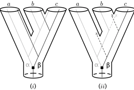
The gene sequences that originate from a gene duplication event are called par-alogs (for example, in Figure2.1(i), the copies α and β for species a). By contrast, orthologous genes are those created from a speciation event (for example, in Figure

2.1(i), the copies α for species b and c).

x x x

a

b

c

!

"

a

b

c

!

"

(i )

(ii )

Figure 2.1: An example of how duplication events can lead to conflict between gene and species trees - Species trees are depicted as thick pipes or tubes and thin lines represent gene trees. Gene losses are represented by an X. (i) the two copies of the gene are available for all species. (ii) the copy α is available for species a and b while the copy β is only available for species c.

Gene duplication can produce conflicts between gene and species trees when some duplicated copies are absent from the analysis, either because they have not been sequenced or because they have been lost at some point during the evolutionary process. For instance, in Figure2.1(ii), the species tree, depicted as thick pipes, says that b and c are closest relatives with respect to a. Suppose that due to losses during the evolutionary process, the only sequences available are the copy α for species a and b and the copy β for species c. In this case, the gene tree (thin lines inside the pipes) groups species a and b, which are not each other’s closest relatives in term of speciation events. This erroneous result comes from the fact that the sequences used to represent species a and b are paralogous with respect to the one used to represent species c. The conflict between gene and species trees due to duplications would disappear if sequences for both copies were available for all species [Doyle,

2.2.2

Horizontal gene transfers (HGT)

Horizontal gene transfer occurs when an organism transfers its genetic material or part of it to a being other than one of its own offspring. Instead, the two or-ganisms are usually unrelated, and are often of different species. Studies of genes and genomes indicate that considerable horizontal transfer has occurred between prokaryotes [e.g.,Jain et al., 1999;Lawrence and Ochman, 1998; Rivera and Lake,

2004]. Indeed, horizontal gene transfer in bacteria is a common phenomenon and is a major factor in accelerating the rate of their evolution [Jain et al., 2003].

There is some evidence that viruses can also transmit genetic information via horizontal gene transfer [Gibbs and Keese, 1995; Pearson, 2008]. The phenomenon appears to have had some significance for unicellular eukaryotes as well. Bapteste

et al.[2005] evoked that «additional evidence suggests that gene transfer might also

be an important evolutionary mechanism in protist evolution». There is some ev-idence that even higher plants and animals have been affected [e.g., Keeling and

Palmer, 2008; Richardson and Palmer, 2007]. However, the prevalence and

impor-tance of HGT in the evolution of multicellular eukaryotes remain unclear [

Huerta-Cepas et al., 2007;Richardson and Palmer, 2007].

a

b

c

x

Figure 2.2: An example of horizontal gene transfer - Species tree is depicted as thick pipes and thin lines represent the gene tree. The gene lineage with its ancestry in species b is transferred in species a.

Horizontal gene transfer is a potential confounding factor when inferring phy-logenetic trees based on the sequence of one gene and can lead to conflicts among individual gene trees. For example, in Figure2.2, the gene lineage with its ancestry in species b is transferred in species a. Since the sequences of species a and b are more similar with respect to that of species c, the gene tree groups species a and b, which are not each other’s closest relatives according to the species tree.

2.2.3

Incomplete lineage sorting

Ancestral polymorphism is the existence of more than one allele, (i.e., alterna-tive DNA sequences at the same physical gene locus), at a locus in an ancestral population. The incomplete lineage sorting is the process by which the ancestral polymorphism is retained through speciation events. This can result in misleading similarities of DNA sequences that do not necessarily reflect species relationships. For instance, in Figure2.3two alleles α and β are present in an ancestral population and both are present after the speciation events. Since the allele α is retained in species a and b while the allele β is retained in species c, the gene tree reconstructed with this gene family sees a and b as each other’s closest relatives while they are not.

! "

a

b

c

Figure 2.3: An example of incomplete lineage sorting - Species tree is depicted as thick pipes and thin lines represent the gene tree. Two alleles α and β are present in an ancestral population and both are retained through speciation events. The allele α is retained in species a and b while the allele β is retained in species c.

2.2.4

Interspecific recombination

Recombination is a molecular process enabling the creation of new combinations of genetic materials through pairing and shuffling of related DNA sequences. Recombi-nation occurs at different levels: individual, population, and species. In prokaryotes and virus, interspecific recombination occurs spontaneously between two organisms. When interspecific recombination occurs, genetic material is exchanged between different species lineages and this can lead to different histories for neighboring segments within a gene [Posada and Crandall,2002;Ruths and Nakhleh,2005]. For instance, in Figure 2.4, species a and c recombined. For the DNA left segment, the gene tree (depicted in thin black lines) is ((b, c), a), but for the segment on the right, the gene tree (depicted in thin grey lines) is ((a, b), c). We can see interspecies recombination as a reciprocal HGT [Ruths and Nakhleh,2005].