Decision-support methodology to assess risk in end-of-life management of complex systems
11
0
0
Texte intégral
Figure
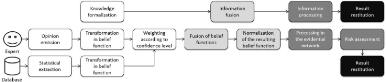
![Fig. 2. Organization of the ERM subprocesses based on [8] and [9].](https://thumb-eu.123doks.com/thumbv2/123doknet/3120998.88691/3.891.138.364.312.521/fig-organization-erm-subprocesses-based.webp)
+2
Documents relatifs