HAL Id: pastel-01065782
https://pastel.archives-ouvertes.fr/pastel-01065782
Submitted on 18 Sep 2014
HAL is a multi-disciplinary open access
archive for the deposit and dissemination of sci-entific research documents, whether they are pub-lished or not. The documents may come from teaching and research institutions in France or abroad, or from public or private research centers.
L’archive ouverte pluridisciplinaire HAL, est destinée au dépôt et à la diffusion de documents scientifiques de niveau recherche, publiés ou non, émanant des établissements d’enseignement et de recherche français ou étrangers, des laboratoires publics ou privés.
non-linéaires par approche expérimentale et design de
contrôleurs robustes: le cas de la cavité ouverte
Claudio Ottonelli
To cite this version:
Claudio Ottonelli. Apprentissage statistique de modèles réduits non-linéaires par approche expérimen-tale et design de contrôleurs robustes: le cas de la cavité ouverte. Mechanics of the fluids [physics.class-ph]. Ecole Polytechnique X, 2014. English. �pastel-01065782�
´
Ecole Polytechnique
Th`ese pr´esent´ee en vue de l’obtention du titre de
Docteur de ´
Ecole Polytechnique
par
Claudio Ottonelli
Apprentissage statistique de mod`
eles r´
eduits
non-lin´
eaires par approche exp´
erimentale et
design de contrˆ
oleurs robustes: le cas de la
cavit´
e ouverte
Soutenue en 20 juin devant un jury compos´e de
F. Lusseyran Directeur de Recherche au CNRS, LIMSI Saclay RapporteurD. Fabre Maˆıtre de Conf´erence, IMFT Toulouse Rapporteur
L. Cordier Charg´e de Recherche au CNRS, PPRIME Poitiers Examinateur L. Pastur Maˆıtre de Conf´erence Universit´e Paris Sud 11 Examinateur
P. Schmid Professeur, LadHyX Palaiseau Directeur de Th`ese
R´esum´e: Cette th`ese est consacr´ee `a la conception d’un contrˆole en boucle ferm´ee d’un ´ecoulement de cavit´e subsonique. L’objectif est de r´ealiser un contrˆoleur qui d´epend seulement de grandeurs observables exp´erimentalement et qui g`ere des situations o`u les ´ecoulements sont excit´es par des perturbations al´eatoires ext´erieures. Pour faire face `a ces deux aspects essentiels, deux strat´egies ont ´et´e d´efinies: l’identification d’un mod`ele non-lin´eaire reproduisant la dynamique de l’´ecoulement `a partir seulement d’informations mesurables et la conception d’un compensateur lin´eaire robuste, bas´ee sur la th´eorie du contrˆole H∞, qui incorpore des propri´et´e de robustesse dans la d´efinition de la fonction
objectif.
La premi`ere partie de la th`ese est consacr´ee `a l’identification d’un mod`ele non-lin´eaire grˆace `a des donn´ees obtenues `a partir d’une exp´erience men´ee dans la soufflerie subsonique (M = 0.1) S19 sur le site Chalais-Meudon de l’ONERA. Afin de d´ecrire la dynamique de cet ´ecoulement, et en particulier son contenu fr´equentiel, l’´ecoulement sans contrˆole a ´et´e caract´eris´e par des mesures par fil chaud et de pression instationnaire et par des clich´es de v´elocim´etrie par images des particules (PIV) r´esolue en temps. Un filtrage temporel a ´et´e appliqu´e avec succ`es aux clich´es PIV afin d’extraire la dynamique basse fr´equence de l’´ecoulement. Cette ´etape est indispensable pour pouvoir g´erer des ´ecoulements turbulents caract´eris´es par un spectre fr´equentiel tr`es ´etendu. Les modes POD obtenus ont ´et´e utilis´es comme base de projection pour le champ de vitesse et les trajectoires associ´ees ont ´et´e interpol´ees (apprentissage statistique) sur une structure de mod`ele non-lin´eaire autor´egressif exog`ene (NLARX). Il s’av`ere que les mod`eles obtenus ne sont pas robustes, dans le sens o`u ils ne parviennent pas `a reproduire la dynamique d’un ensemble de donn´ees de validation, une fois adapt´es `a un ensemble de donn´ees d’apprentissage. Il a ´et´e d´emontr´e que cet ´echec est dˆu aux fortes non-lin´earit´es observ´ees dans l’´ecoulement de cavit´e, qui rendent impraticables les m´ethodes d’identification.
La deuxi`eme partie de la th`ese est consacr´ee `a la conception d’un contrˆoleur robuste `a partir de simulations num´eriques d’un ´ecoulement de cavit´e carr´ee, incompressible et en r´egime transitionnel, pour diff´erents nombres de Reynolds. Diverses m´ethodes de synth`ese de contrˆoleur ont ´et´e test´ees et ´evalu´ees en utilisant plusieurs mesures de robustesse. On a constat´e que la technique traditionnelle de contrˆole lin´eaire quadratique gaussien (LQG) pr´esente une faible robustesse aux perturbations ext´erieures, tandis que d’autres, comme la technique LTR (Loop Transfer Recovery) et les contrˆoleurs bas´es sur les perturbations “les pires” (worst-case), am´eliorent la robustesse, mais pas suffisamment pour faire face `a la forte non-lin´earit´e de l’´ecoulement. Dans ce but, on met en place un contrˆoleur qui optimise les propri´et´es de robustesse par rapport `a des incertitudes de type “entr´ee-multiplicative” et de type “entr´ee vers sortie”. Celui-ci pr´esente des marges de robustesse fortement augment´ees par rapport `a l’introduction de perturbations de la partie stable de la dynamique entr´e-sortie, mˆeme si le prix `a payer en terme de performance est significatif. Une strat´egie pour prendre en compte ´egalement des perturbations de la partie instable de la dynamique entr´ee-sortie, comme celles obtenues par un changement du nombre de Reynolds, a ´et´e pr´esent´ee.
Mots cl´es: cavit´e, contrˆole d’´ecoulement, boucle ferm´ee, r´eduction de mod`ele, modes POD, projection Galerkin, identification de syst`eme, robustesse, incertitudes non struc-tur´ees.
and that handles situations where the flow field is excited by unknown external random disturbances. For this, two strategies have been defined: the identification of a non-linear model representing flow dynamics from only measurable information and the design of a robust linear compensator, based on the H∞ control theory, that incorporates robustness
properties in the objective function definition.
The first part has been devoted to the identification of a non-linear model with data obtained from an experiment conducted at the ONERA S19 subsonic (M = 0.1) wind tunnel on the Chalais-Meudon site. In order to provide a full description of the fluid motion, in particular its frequency content, the natural (without control) flow has been characterized by hot-wire and unsteady pressure measurements and time-resolved Particle Image Velocimetry (PIV) snapshots. Time-filtering has been successfully applied to the PIV snapshots in order to focus on the large-scale low-frequency dynamics of the flow. This step has been shown critical to deal with turbulent flows characterized by high-frequency noise. The obtained POD modes have been used as a projection basis of the velocity field and the associated trajectories fitted to a Non-Linear Auto-Regressive eXogeneous (NLARX) model structure by an identification process. It turns out that the obtained models are not robust, in the sense that they do not manage to reproduce the dynamics of a validation data-set once fitted to a given learning data-set. It has been shown that this failure is due to the strong non-linearities observed in the cavity flow and that render identification methods impracticable.
The second part has been devoted to the design of a robust controller from numerical simulations of an incompressible square cavity flow at different Reynolds numbers in transitional regime. Various control design methods have been tested and assessed with respect to several robustness measures. It was found that the traditional Linear Quadratic Gaussian (LQG) controller exhibits poor robustness to external perturbations and that loop-transfer recovery (LTR) techniques and “worst-case” controllers improve robustness but not sufficiently to cope with the strong non-linearities in the flow. To this aim, a compensator design that optimizes the robustness properties with respect to unstructured input-multiplicative and input-to-output uncertainties is presented. The latter shows an important increase in robustness with respect to the introduction of perturbations of the stable part of the input-output relation even though a cost is payed in terms of performances. A strategy to deal also with perturbations of the unstable part of the dynamics, as obtained for example by change in Reynolds numbers, has been introduced.
Key words: cavity, flow-control, feedback, model reduction, POD modes, Galerkin projection, system identification, robustness, unstructured uncertainties.
Contents
1 Introduction 1
1.1 Subsonic cavity flow . . . 1
1.2 Closed-loop control . . . 3
1.3 Model reduction . . . 5
1.4 System identification . . . 7
1.5 Robust control . . . 8
1.6 Objective of the thesis and outline . . . 9
1.6.1 Outline . . . 10
2 Experimental activity 13 2.1 Wind tunnel qualification . . . 14
2.1.1 Hot-wire measurements . . . 15
2.1.2 Pressure measurements . . . 17
2.1.3 Frequency adaptation . . . 19
2.2 Time-Resolved PIV . . . 20
2.2.1 The PIV technique . . . 21
2.2.2 TR-PIV measurements . . . 21
3 Non-linear model identification 25 3.1 Non-linear reduced models . . . 26
3.1.1 Proper orthogonal decomposition . . . 26
3.1.2 Galerkin projection . . . 27
3.1.3 System identification . . . 28
3.2 POD from TR-PIV . . . 29
3.2.1 POD modes and trajectories . . . 29 i
3.2.2 Time-filtering . . . 30 3.2.3 Summary . . . 36 3.3 NLARX model . . . 36 3.3.1 Model description . . . 37 3.3.2 Model learning . . . 38 3.3.3 Model validation . . . 39 3.3.4 Critical analysis . . . 40
4 Robust feedback control of a cavity flow 43 4.1 Flow configuration . . . 44
4.1.1 Flow configuration . . . 44
4.1.2 Governing equations . . . 45
4.1.3 Actuator and sensor definition . . . 46
4.2 Model reduction . . . 47
4.2.1 Global modes . . . 48
4.2.2 Balanced POD modes . . . 50
4.2.3 Summary . . . 52
4.3 Closed-loop system . . . 52
4.3.1 Closed-loop transfer function . . . 53
4.3.2 Closed-loop perturbations . . . 54
4.4 Performance and robustness definition . . . 54
4.4.1 Performance definition . . . 54
4.4.2 Classic robustness definition . . . 56
4.4.3 Unstructured uncertainty . . . 58
4.4.4 Summary . . . 61
4.5 Control design targeting performance . . . 62
4.5.1 LQG in small gain limit hypothesis . . . 63
4.5.2 Loop transfer recovery . . . 67
4.5.3 H∞ control . . . 72
4.6 Control design targeting robustness . . . 74
4.6.1 Input-multiplicative perturbation . . . 76
4.6.2 Input-to-output perturbation . . . 79
4.7 Unstable perturbations . . . 80
5 Conclusions 85 5.1 Perspectives . . . 87
CONTENTS iii
Chapter 1
Introduction
Active flow control played in the very last decades a key role in the suppression of flow-field unsteadiness that are the main cause of noise, structural vibrations, drag increase and a number of issues in a large range of industrial applications. The interest in this area led to a development of technological devices, actuators and sensors, and control methodologies focused to manipulate the greatest range of flows as reviewed by Cattafesta and Sheplak (2011).
Among different types of control strategies — active, passive, open-loop, closed-loop, etc — active closed-loop control in fluid flows has received a lot of attention in recent years, in particular from the aerospace industry. The advantage of this kind of control is the small amount of energy input, compared to open-loop control, with the possibility to strongly alter the flow dynamics.
However, closed-loop control implies different approaches among control theorists and experimentalists, since the first often ignore the practical limitations imposed by the the existing technology and, on the other hand, the latter often do not appreciate dynamic requirements imposed by feedback control.
The study and analysis presented in this thesis are part of the closed-loop control of unsteady flows. In particular, they focus on the establishment of theoretical control methods applicable under experimental conditions.
1.1
Subsonic cavity flow
Flows over open cavities have been deeply studied by control theorists, fluid dynamicists and aeroacousticians, because of the variety of characteristics of such flows. The need to model different scales of aero-acoustic disturbances, to control competing modes in a large range of different conditions represent a challenge not always accomplished. For these and a number of other reasons, the flow over an open cavity is considered as a canonical problem in flow control.
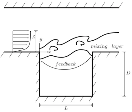
x y δ mixing layer f eedback L D
Figure 1.1: Schematic description of the cavity resonance.
The dynamics of separated flows are of fundamental interest in a number of realistic configurations. Kelvin-Helmholtz instabilities are commonly present in this type of flows causing an unsteady behavior in the shear-layer of the separation bubble. It is then of a great interest to suppress or weaken its unsteadiness. The open-cavity flow is a prototypical example of sustained instability. This type of flow exhibits a recirculating component (confined geometrically to the cavity) as well as a strong shear layer that forms at the top of the cavity and, for sufficiently high Reynolds numbers, becomes unstable and settles into a characteristic periodic motion (Sipp and Lebedev, 2007).
The control framework depends on the nature of the flow to be controlled. Globally unstable flows are more easily controlled, because of the limited number of structures at well-defined frequencies. The techniques applied in these situations have greatly relied on a mathematical framework established in control theory as described in standard references (Burl, 1998; Zhou et al., 1996), but additional complications had to be overcome when adapting them to fluid flows.
Cavity flows are characterized by a self-induced beating at a particular frequency. This behavior is typical for oscillating flows (Huerre and Rossi, 1998) and it consists in an exponential amplification of a given perturbation of the flow field followed by its saturation due to non-linear effects. The flow-induced cavity resonance mechanism is schematized in Fig. 1.1. A boundary layer of thickness δ separates at the upstream corner of a cavity of length L and depth D. The mixing layer develops over the cavity and eventually reattaches near the downstream edge. The downstream wall acts as an acoustic source, and the generated waves travel upstream. The acoustic waves force the shear layer at the
1.2. CLOSED-LOOP CONTROL 3
upstream edge as a feedback process producing resonant frequencies.
The mechanism has been described by Rossiter (1964) and is influenced by geometric parameters (L and D) and flow conditions (M and Re). Each flow is then characterized by specific cavity tones and the following harmonics. For this reason, cavity flows have been the subject of a huge quantity of studies since the late ’50s. An exhaustive review of simulations, modeling and active control of flow/acoustic resonance in flows over open cavities can be found in Colonius (2001).
1.2
Closed-loop control
Flow control is necessary in a number of engineering applications and consists in the alteration of the original state towards a desired condition. Two strategies can be distin-guished, passive control and active control. In this study we focus on the latter and, in particular, to closed-loop active control. However, an overview of flow control is given.
In aeronautic industry, passive control has played, and still plays, an important role, since it does not require any energy input. It consists in the alteration of the flow through geometric modifications or by placing artifacts in specific regions. Relevant examples of these devices and solutions are: vortex generators used to enhance turbulence in boundary layers (Godard and Stanislas, 2006) and therefore to delay separation (for drag reduction purposes) (Aider et al., 2010; Pujals et al., 2010), surface riblets used to reduce skin friction in channel flows (Walsh, 1983; Baron et al., 1993; El-Samni et al., 2007) and cylinders or rods placed near the leading edge of a cavity to suppress resonances (McGrath and Shaw, 1996; Illy et al., 2008; Yamouni et al., 2013).
Although good results have been shown by passive control techniques in particular conditions, a lack of adaptability and robustness to changes in flow conditions has been also remarked and represents a huge limitation. Technology evolution allowed the devel-opment of active control strategies capable to deal with these situations in a wider range of applications.
The peculiarity of active control is the need of energy and a more complex system in order to adapt to flow changes. The amount of energy requested has to be compared with a global advantage in terms of energy saving or power gain, as explained by Kasagi et al. (2009). In practical aeronautical applications, an example can be represented by control techniques designed for skin-friction drag reduction, that has the consequence of a diminished fuel consumption. Active control can be performed with two different strategies: closed-loop control, where the control law is defined from feedback given by real-time measurements, and open-loop control, that relies on no feedback.
Open-loop control lived its golden era in particular during the 90s and the first years of the 2000s. Many applications have been the objective of this technique, as the suppression
Ref. Error
Control Control Input P lant
Disturbance
Output
F eedback
−
Figure 1.2: Closed-loop control scheme. Each block represents a transfer function, while the arrows are related to time-domain quantities.
of cavity resonances or the reduction of viscous drag. To these aims, a wide set of actua-tion devices has been employed: oscillating electromechanical and piezoelectric flaps and plates, fluidic oscillating jets, voice-coil drivers, steady and pulsed blowing and resonance tubes, as reviewed in Cattafesta et al. (2003). Successful results in active open-loop flow control have been obtained by Zhuang et al. (2006) and Ukeiley et al. (2007) on cavity tones suppression and by Quadrio and Ricco (2004) on drag reduction from span-wise wall oscillations.
Closed-loop control became more important with the development of real-time tech-nologies. The key feature of the closed-loop control is that some flow quantities, measured or estimated, are fed back to an algorithm that modifies the optimal control signal that minimizes a prescribed objective (Di Stefano et al., 1990). A simple representation of the feedback system is schematized in Fig. 1.2, where sensors and actuators are included in the plant, without specification of the frequency contribution.
A huge importance in feedback control is then assumed by actuators and sensors. Their performances and efficacy are evaluated in terms of static and dynamic responses, energy requirement, size, weight, bandwidth, gain (for actuators) and sensitivity (for sensors). These characteristics have the same importance than the fluid interaction. Typically, in feedback flow control, actuation devices are: piezoelectric moving flaps, zero-net mass flows and plasma actuators. Sensors used more frequently in this type of applications are generally unsteady pressure transducers, hot wires and hot films and thermocouples. These devices present good features in terms of frequency bandwidth and time response. The main characteristics and design issues for actuators and sensors are summarized in a number of reviews as Cattafesta and Sheplak (2011).
The information given by sensors can be used with two different approaches: quasi-static and dynamic controllers. The first closed-loop strategies were modifications of open-loop control techniques. For instance, feedback has been used in several works to slowly tune the frequency of an open-loop forcing to improve the suppression of unsteady
1.3. MODEL REDUCTION 5
pressure oscillations or the reduction of velocity fluctuations. These kind of controllers are called by Cattafesta et al. (2003) “quasi-static” since the feedback dynamic is much slower than flow dynamics. Notable examples in cavity flows are represented by Shaw and Northcraft (1999), that modulated a sinusoidal forcing function to reduce the sound pressure level of cavity resonance, and by Debiasi and Samimy (2004), that used an adaptive algorithm to adjust the frequency forcing. More recently, and more interesting for our purpose, are the “dynamic” controllers, where the feedback dynamics have the same time-scale of the flow dynamics.
Real-time controllers are designed from the application of the control theory and ap-plied to systems representing flow dynamics. This process can represent a huge difficulty due to the variety of features of each discipline, control theory and fluid mechanics. Be-wley (2001) pointed out the importance of having a deep knowledge of both areas and capitalize technological and theoretical development in order to deal with problems arising in the research field. With this spirit, different control techniques have been developed and successfully applied to both numerical and experimental flows.
In this study, active closed-loop control has been attempted to suppress cavity oscil-lations. Closed-loop control methodologies applied to cavity problems need a model that represents the most important dynamics. The quality of the model depends on the num-ber of sensor measurements, their location in the cavity and their capacity to capture flow information. Many different modeling techniques have been used in recent years, either based on flow physics or empirically identified directly from an experiment. The most used techniques are system identification and projection methods, but also physics-based models as in Rowley (2005).
1.3
Model reduction
The substitution of the high dimensional problem with a reduced model leads to an easy optimization of the control law. Thus, the latter depends on how flow dynamics are represented in the model. One of the most important objective of flow control is then to obtain a reduced model that, in spite of low dimension, is capable to accurately reproduce the input-output dynamics.
In the majority of studies on transitional flow control, linear models have been consid-ered to represent the dynamics of the linearized Navier-Stokes equations, as reviewed in Kim and Bewley (2007). The hypothesis of applicability is that linearized models faith-fully reproduce input-output dynamics and in the last decade this hypothesis has been widely supported, at least at sufficiently low Reynolds number. Clearly, the limit of such models is the inability to capture turbulent dynamics related to different length and time scales, typically non linear. On the other hand, a non-linear approach can be effective
even in super-critical conditions (Bergmann and Cordier, 2008). Independently from the approach, a reduced model musts rely on a discretization of the high-dimensional prob-lem. In this thesis, we consider reduced basis approaches, that consist in the projection of the flow equations onto a low-dimensional basis reproducing some important features of the input-output dynamics. In particular, we focus on Global Modes (GM), Proper Orthogonal Decomposition (POD) and balanced POD (BPOD).
Model reduction can be obtained by projection of the high-dimensional problem onto global modes. These modes are computed in the stability analysis and represent the eigenvectors of the linearized Navier-Stokes operator (Sipp et al., 2010). Due to their non-orthogonality, an adjoint basis, obtained through the solution of the adjoint Navier-Stokes operator, is also required. Through a linear combination of global modes, full system’s linear dynamics can be accurately expressed. A reduced model from projection onto global modes has been used in boundary-layer flows to model optimal perturbations and linear growth in the works of ˚Akervik et al. (2008), Ehrenstein and Gallaire (2005) and Alizard and Robinet (2011). Since global modes are related only to system dynamics, Lauga and Bewley (2004) observed that with the introduction of measurements and forc-ing, global modes expansion is no longer appropriate to capture the modified dynamics. However, closed-loop control using reduce-order models obtained with this method have been studied in ˚Akervik et al. (2008) and Ehrenstein et al. (2012). Barbagallo et al. (2009) used the least stable modes as basis for the reduced-order model.
Control approaches in recent years have been developed on reduced-order models mostly based on Proper Orthogonal Decomposition (POD) method. This technique has the objective of obtaining a low-dimensional orthonormal basis, so that the velocity field can be expressed as a linear combination. This technique is well suited for fluid mechan-ics problems (Lumley, 1967), since it does not require any information of the flow, but relies only on snapshots of the velocity field, that can be easily obtained from numerical simulations as well as experimental PIV acquisitions. This method turns into solving an eigenvalue problem, whose size is equal to the number of snapshots (Sirovich, 1987), from a correlation term computed as a scalar product of the velocity field. Resulting eigenmodes (POD modes) represent the most energetic structures that can be controlled and their dynamics are modulated by time projection of the velocity field onto the POD basis. Model reduction with POD has been applied to numerous works to describe the energy-based dynamics as in Noack et al. (2003) and Rowley et al. (2004). This spatial decomposition technique is usually coupled with Galerkin projection, leading to the class of methods called Galerkin-POD methods, widely used in flow control. Successful results in this domain can be found in the works of Bergmann and Cordier (2008) on a cylinder wake, Barbagallo et al. (2009) on a cavity flow and in the experimental work of Samimy et al. (2007).
1.4. SYSTEM IDENTIFICATION 7
A further step in POD-based model reduction consists in balanced truncation. It is recognized that to reduce the order of the problem, both controllabilty, i.e. the ability of the applied forcing to reach flow states, and observability, i.e. the ability of flow states to register at the sensor locations, are equally important. Moore (1981) first introduced a model reduction where the basis balances these two characteristics and he applied it to systems linearized about stable steady states. In flow control a similar basis is well suited to represent the information from the actuator to the sensor providing a reduced model subjected to optimal control design. These balanced models were also consequently applied to unstable systems (Zhou et al., 1999) and non-linear control problems (Scherpen, 1993; Lall et al., 2002). More recently, Rowley (2005) combined the balancing procedure and Proper Orthogonal Decomposition (POD) modes. Since then, this technique has been applied to channel flows (Ilak and Rowley, 2006; Ahuja and Rowley, 2008; Ilak and Rowley, 2008) and boundary layer problems (Bagheri et al., 2009; Ahuja and Rowley, 2010). For the cavity flow problem we refer in this study to the balancing procedure and detailed results provided by Barbagallo et al. (2009).
1.4
System identification
In flow control, the process of going to observed data to a mathematical model is called System Identification (Ljung, 1999). This technique covers the problem of building a model when previous history is barely known and only dynamics features are available. The resulting model can be then considered as a black box between the actuator and sensor that, accordingly to Kim and Bewley (2007), are the only dynamics required for compensator design. For this reason, system identification provides models that are well suited for control in experimental applications. Some successful examples in this domain are the work of Kegerise et al. (2004) on the suppression of flow-induced cavity tones, the adaptive control of a separated boundary layer made by Tian et al. (2006), the closed-loop control of the reattachment length downstream of a backward-facing step by Henning and King (2007), the suppression of the gust effect on an airfoil studied by Kerstens et al. (2011) or the approximation of linearized Navier-Stokes equations through system identification obtained by Herv´e et al. (2012).
The range of different techniques to obtain an identified model is wide and new solu-tions have been continuously proposed in recent years. In this research we focus on those techniques where the model describing input-output behavior is obtained from projection onto Navier-Stokes equations. Commonly, this procedure is applied to flow equations linearized around a steady base flow. The techniques of this type most used recently are Auto-Regressive eXogenous (ARX) models (Huang and Kim, 2008), in which the error is modeled as a white noise, and Auto-Regressive Moving-Average eXogenous (ARMAX)
models (Herv´e et al., 2012), where a colored noise is considered in the algorithm without an a priori knowledge of the color. Despite the technique used, the system identification procedure can be summarized as follows. From the available measurements and inputs, a set of candidate models is analyzed. A model is a predictor of the next output from the process, given past observations and a set of parameters. The structure of the model thus depends on the dynamics of the flow to be represented and results as a combina-tion of constant coefficients, to be determined, and time regressors, i.e. combinacombina-tion of past measurements and inputs. Because of unpredictable dynamics, the next output is approximated with an unknown error. Constant coefficients can be computed through a least-square method that minimizes this error. The model obtained is then tested on a different set of data.
An alternative is represented by the identification of linear system matrices, known as subspace identification and first introduced by Kalman (1960). This technique is widely used in control problems based on Linear Quadratic Gaussian (LQG) regulators, since it provides an approximation of the noise covariance as required in control design. On this matter, Juillet et al. (2013) proposed a technique for evaluating a combined approach involving subspace identification and optimal control design. Among other closed-loop subspace identification methods, we can cite the work of Chiuso and Picci (2005) on the consistency of two different subspace identification methods based on a whitening filter approach and the error estimation approach from a high-order ARX model proposed by Qin and Ljung (2003). A more detailed review of methods based on subspace identification technique can be found in Qin (2006).
1.5
Robust control
Linear-quadratic optimal regulators have impressive robustness properties, including guar-anteed classical gain margins. This result is only valid, however, for the full-state case. If observers or Kalman filters are used in the implementation, no guaranteed robustness properties hold. In light of these observations, the robustness properties of control systems with observers need to be separately evaluated for each design.
The present study provides procedures to directly target robustness. Loop Transfer Recovery (LTR) technique already improves robustness in the Linear Quadratic Gaussian (LQG) regulator by adding a fictitious control noise. Cortelezzi and Speyer (1998) intro-duced the Multi-Input-Multi-Output (MIMO) LQG/LTR synthesis, combined with model reduction techniques, for designing an optimal linear feedback controller. Among robust regulators, the H∞ control has been introduced by Doyle et al. (1989). It consists in a
worst-case disturbance (min-max) problem where the objective is to find the particular disturbance to which the compensator is most sensitive and nonetheless the amounts of
1.6. OBJECTIVE OF THE THESIS AND OUTLINE 9
feedback are kept as small as possible. A worst-case disturbance (H∞) controller has been
developed by Bewley and Liu (1998) to stabilize unstable disturbances in transitional flow. Such reduced feedback improves robustness in the system model and results in a smaller demand on the actuator. The problem of finding a robust control is intimately coupled with the problem of finding the worst-case disturbance in the spirit of a non-cooperative game. The cost functional is simultaneously maximized by the disturbance and minimized by the control. The principle behind the robust control theory could be intuitively seen as a compromise seeking the “best” control that stabilize the flow, between the smallest control effort and the worst effect done by disturbances. A control which is effective even in presence of a worst-case disturbance will be robust to a wide range of other possible disturbances.
In the present study a H∞ controller is developed considering unstructured
uncer-tainties as disturbances, as described by Burl (1998). This type of perturbation can be related to the internal stability robustness through the Small Gain Theorem (SGT) leading the H∞ controller to directly target robustness instead of performance. This
ap-proach is known in control community as the input-output apap-proach and is one of the well-accepted and widely-used methods to study stability of systems. Initiated by Zames (1966), the small gain theorem says that the feedback loop will be stable if the loop gain is less than one. This simple rule has been a basis for numerous stabilization techniques in control theory. However, the application of this method cannot be found in flow control problems.
1.6
Objective of the thesis and outline
In this work, two key points of closed-loop control applications are investigated: model reduction through system identification based on observable dynamics and robustness to stable perturbations. The aim is to build a controller suited for experimental applica-tions. With this purpose a subsonic, bi-dimensional cavity flow has been studied through experimental activity and numerical simulations.
As described in Sec. 1.4, system identification technique has been successfully applied to closed-loop linearized control problems. In particular, auto-regressive models permit to predict the measurable output through a linear combination of previous acquisitions and known inputs. However, real applications can be found only for transitional flows at low Reynolds number where non-linear effects are not predominant. Dealing with these non-linearities in real cases is a challenge that can be engaged with an approach based on the system identification technique. This is the first purpose of this thesis, the realization of a non-linear identified model based on experimental acquisitions. The expectation is that such a model could deal with the oscillating behavior of the cavity flow.
Optimal control theory has been widely used in flow control applications. However, many aspects and features of control theory are not considered in fluid mechanics prob-lems that have been historically focused on classical control methods as linear quadratic control. The reason of this “lack of communication” between control and fluid mechan-ics communities is that the two disciplines have been tied together only in the last two decades and, even though many progresses have been accomplished, the huge potential of control theory has not been fully exploited in flow control. An example is represented by the input-output approach, a technique deeply employed in automatic control to stabilize feedback systems and almost unknown in fluid mechanics domain. The main objective of the present work is then to build a controller based on this technique in order to increase robust behavior to stable perturbations showing that modern automatic control methods can be suited even for flow control applications and can lead to impressive results.
1.6.1
Outline
This thesis is structured as follows: a first part where a real case has been analyzed through an experimental activity and a second part in which robust control is developed from numerical simulations.
In chapter 2 the experimental activity conducted on the S19 wind tunnel is described. The equipment is functional to perform closed-loop control. The qualification measure-ments are highlighted in Sec. 2.1, focusing on hot-wire measuremeasure-ments, steady and unsteady pressure acquisitions. Particular emphasis is given to frequency content. PIV technique has been used to give a time-resolved description of the flow dynamics and its principle, along with qualitative results, is shown in Sec. 2.2.
The identification of a non-linear reduced-order model is the main subject of chapter 3. Non-linear models are introduced in Sec. 3.1, where the structure of the identification algorithm is defined from a POD basis. TR-PIV measurements are then used to compute POD modes and time projections in Sec. 3.2. In this section, great relevance is also given to time-filtering process over PIV snapshots. Finally, the different phases of the identification process are described in Sec. 3.3, with a detailed analysis on the role of each parameter.
Closed-loop robustness analysis is conducted in chapter 4. Numerical simulations and model reduction are described in Sec. 4.1 and 4.2. The definition of the closed-loop system is given in Sec. 4.3. Here, key roles are represented by the closed-loop transfer functions and perturbations. In the following Sec. 4.4, performances and robustness indicator are defined. These quantities represent the comparison parameters for the control strategies studied. A new interpretation of robustness to stable perturbations is also given. In Sec. 4.5 results of classic control strategies as LQG, LQG/LTR and classic H∞ control are
1.6. OBJECTIVE OF THE THESIS AND OUTLINE 11
4.6. Finally, the behavior to unstable perturbations of the most robust compensator is analyzed in Sec. 4.7, with considerations of future perspectives.
Chapter 2
Experimental activity
In this chapter, we describe the experimental activity carried out in the continuous closed-loop subsonic (M a ≈ 0.1) wind tunnel “S19Ch”, on the Chalais-Meudon site. We aim at performing a real feedback control capable of suppressing cavity oscillations. To this purpose, the control strategy will consider the possibility of using unsteady measurements, such as “traditional” sensors (pressure probes, hot wires and hot films), as well as time-resolved PIV images. The equipment installed on the wind tunnel has been devised for this objective.
The model mounted in the S19Ch wind tunnel is represented in Fig. 2.1. It consists of a cavity of length L = 134mm, original depth Do = 210mm (then modified to Dm = 900mm
in order to modify the fundamental frequency of the cavity) and span W = 300mm. Reference conditions measured upstream the cavity, are closed to ambient temperature and pressure: Tref = 293.7 ± 10K and Pref = 100383 ± 600P a. The related Reynolds
number is then Re ≈ 105.
The experimental setting is equipped with an acquisition system that simultaneously acquires 16 different channels of measurement. Among these, 7 channels are dedicated to unsteady pressure acquisitions; 3 are for relative steady pressure Ptotal − Patmospheric
and Pstatic− Ptotal measured upstream the cavity and Pstatic− Patmospheric measured at 28
points along the vein; 1 for a hot-wire probe that could be displaced through a system capable to cover an area of 25cm in the streamwise direction and 10cm in the vertical direction; 2 channels for temperature acquisitions of Tref and Ttotal. Remaining channels
have been eventually used for tests and minor purposes.
To obtain time-resolved PIV snapshots (to have a description of the flow dynamics, to build reduced order models and to be used as sensors in a closed-loop control scheme), a high-frame rate camera and a double cavity laser have been installed. The observation window of 1280×500 pixels is focused only on the shear layer, giving a description of the oscillating motion, but the recirculating dynamic on the bottom of the cavity is not captured.
Figure 2.1: Cavity model installed in the S19Ch wind tunnel.
A field-programmable gate array (FPGA) has been included to quickly process infor-mation between the TR-PIV system, the actuator (here a low-frequency flap) and the unsteady pressure measurements. In the perspective of closed-loop control, considering the low characteristic frequency of the cavity flow and consequently the low operating fre-quency of the actuator, the process of analysis and impulse granted by the FPGA system can be considered approximately as real-time process.
The chapter is structured as follows: in Sec. 2.1, measurement techniques and quali-fication results are presented. These measurements are useful to characterize the flow in terms of boundary layer width, pressure, turbulence intensity and frequency bandwidth, in order to provide the parameters needed for the PIV campaign and the actuator design. Results of TR-PIV are presented in Sec. 2.2. In particular, time resolution permits a high detail of information as small structures displacement and vorticity evolution, within a characteristic period.
2.1
Wind tunnel qualification
In this section we analyze measurements conducted at the wind tunnel S19Ch in order to qualify the vein. The cavity model has been conceived and installed for this specific study and for this reason no reference data was available. Hot-wire measurements in the boundary layer and the free shear layer and pressure measurements, both steady and unsteady pressure, have helped to characterize the flow over the cavity and to modify the geometry in order to have lower and more manageable frequencies.
2.1. WIND TUNNEL QUALIFICATION 15 0 5 10 15 20 25 0 0.2 0.4 0.6 0.8 1 1.2 0 0.001 0.002 0.003 0.004 0.005 y U / U0 σ 2/ U 2 0 (a) 101 102 103 0 10 20 30 40 50 60 U + y+ U+= 1 0.25ln(y +) + 8 (b)
Figure 2.2: (a) Wall normal evolution of the normalized velocity (circles) and the related variance (diamonds). (b) Scaled velocity in wall units.
2.1.1
Hot-wire measurements
Hot-wire anemometry technique is mostly used to measure turbulence in air flows and it is based on a heat/convection correlation principle. A very thin wire, generally made of tungsten, of diameter ∼ 0.5 to 5 µm and length 0.3 to 1 mm, when placed in a flux of air, changes its temperature and so its resistance. Most hot-wires operate at constant temperature, so the change of air velocity causes an increment in the voltage necessary to keep the temperature constant. This imbalance is measured by the data acquisition system and converted by a calibration law to a local velocity.
In the wind-tunnel qualification campaign, the hot-wire technique has been used to obtain a measurement of the upstream boundary layer profile, to characterize the cavity flow frequency and to compute the turbulence level in the flow.
Boundary layer
The upstream boundary layer is measured with a Dantec 55P15 probe, that permits with its specific geometry to approach the wall up to 0.5 mm. Measurements are taken in the upstream region, with the cavity closed in order to have no acoustic disturbance. Re-sults are represented in Fig. 2.2. The first plot (Fig. 2.2(a)) shows the evolution of the normalized velocity U/U0 in the direction normal to the wall, y, and the corresponding
non-dimensional variance. This measurement allows to compute boundary-layer thick-ness: the 99% thickness δ.99 = 21.24mm, the displacement thickness δ∗ = 3.35mm, the
momentum thickness θ = 2.55mm and the shape factor H = 1.31.
The second plot, shown in Fig. 2.2(b), presents an evolution of the boundary layer in estimated scaled wall units. Since it is not possible to compute the exact value of the velocity very close to the wall, the viscous velocity has been estimated to have unitary value. Results show only the buffer layer around y+ = 10, the log-law region from y+ =
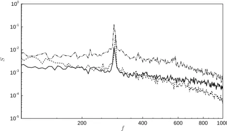
200 400 600 800 1000 10-5 10-4 10-3 10-2 10-1 100 S f
Figure 2.3: Spectra of measured signals (in V ) at three different locations in the cavity: x = 4mm, y = 0mm (solid line), x = 60.7mm, y = −25mm (dashed line) and x = 130mm, y = 0mm (dashed-dotted line).
because of the limits of the hot-wire technique when approaching the wall. Note that the logarithmic behavior is well represented, but since the scaling is just estimated, the describing law shows a value of the Von K´arm´an constant quite different from the classic 0.41.
Mixing layer
The mixing layer has been investigated by displacing a Dantec 55P11 hot wire through an explorer mounted on the top of the cavity, with the flow nominally driven at 40m/s. The region investigated by the hot-wire probe is a rectangle of 21 points in the longitu-dinal direction, starting at 4mm from the upstream edge of the cavity to 4mm to the downstream edge, and 6 points in the normal direction, from y = 0mm to −25mm inside the cavity. These measurements have been used to characterize the frequency range of the cavity. In Fig. 2.3 we observe three spectra of the anemometer acquisition at three different locations: two points close to the upstream and the downstream edge and one inside the cavity in the recirculating region. Near the corners, the spectra presents a peak at 288 Hz, while at the lowest location the peak is located at 293 Hz. This small difference is due to the lack of resolution, since the hot-wire signal is acquired at 20 kHz and composed of 4096 points and the passage to the frequency domain implies a Fourier transform that leads to a frequency step of 4.88 Hz.
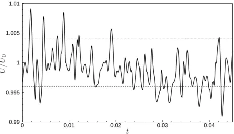
2.1. WIND TUNNEL QUALIFICATION 17 0 0.01 0.02 0.03 0.04 0.99 0.995 1 1.005 1.01 t U /U 0
Figure 2.4: Time behavior of a normalized velocity signal acquired with a hot-wire probe located in the free stream.
Turbulence intensity
The quality of a wind-tunnel flow is commonly expressed by the turbulence intensity, also often referred to as turbulence level, defined as:
I ≡ u¯′
U, (2.1)
where u′ is the root-mean-square of the turbulent velocity fluctuations and ¯U is the mean
velocity. It represents how statistically a flow fluctuates around its mean value, so it is a good representation of how “clean” the flow in a wind tunnel is and it can be easily calculated from a hot-wire acquisition, knowing the mean value and the variance. For this wind tunnel, the turbulence level is I ≈ 0.4% and it is a typical value for high-quality wind tunnels.
In order to better understand the meaning of the turbulence level we can observe Fig. 2.4 where a normalized velocity signal measured in the free stream is represented. The horizontal lines stand for the bounds of the 0.4% of the normalized velocity. We can note how the majority of the oscillations are included between these bounds.
2.1.2
Pressure measurements
The S19 wind-tunnel is equipped with 26 static pressure probes and 7 unsteady pressure Kulite transducers. In this section we show results for both measurement techniques.
0 500 1000 1500 -1000 -900 -800 -700 -600 x P
upstr. cav. downstream divergent
Figure 2.5: Steady pressure measurements along the model section. Pressure values are expressed in P a, while the longitudinal direction is in mm. Top static probes are repre-sented by squares, bottom probes by circles.
Steady pressure measurements
A series of static pressure probes has been posed along the wind tunnel, from a location 184 mm upstream the cavity to the divergent section, placed on top and on bottom of the vein. Fig. 2.5 shows the longitudinal behavior of the static pressure, with respect to the atmospheric pressure. There is no remarkable difference between the top and the bottom acquisitions, as expected, except for the probes located on the cavity vertical walls. In detail, there is a significant jump in pressure inside the cavity at the upstream wall, while on the downstream wall this jump is not present. The static pressure continues to diminish along the x direction until the divergent region where the flow is finally decelerated.
Unsteady pressure measurements
Unsteady pressure acquisitions are taken from 7 Kulite transducers XCQ-093-15A (15 PSI). Two of them are positioned on the upstream wall of the cavity, four on the down-stream wall and one on the bottom. From these acquisitions it has been possible to obtain a power spectra of the cavity, verify that the flow is actually two-dimensional and com-pare results with those obtained with the hot-wire anemometer. The advantage of using this kind of transducers is a high sampling frequency, here 20kHz, for 200 blocks of 4096 points, giving a frequency resolution of 4.88 Hz.
In Fig. 2.6 is shown the Sound Pressure Level (SPL) obtained from the power spectra of three different Kulites, one at the upstream wall, one at the downstream wall and one
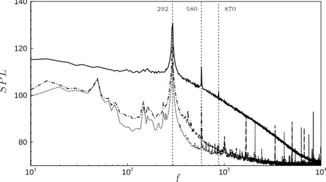
2.1. WIND TUNNEL QUALIFICATION 19 101 102 103 104 80 100 120 140 292 580 870 f S P L
Figure 2.6: SPL, expressed in dB, of unsteady pressure measurements. Transducers are located on the upstream wall of the cavity (dashed line), on the downstream wall (solid line) and on the bottom (dashed-dotted line).
at the bottom wall. The SPL is computed through the relation SP L(dB) = 20 log10 √ S pref ! (2.2) where S is the power intensity of the pressure measurement and pref is the reference
pressure equal to 20µP a that is considered as the threshold of human hearing. We can observe that all the signals present a peak at 292Hz and the second and third harmonics are located at 580 and 870Hz. Comparing this result with that obtained from the hot-wire probe we can define the characteristic frequency of the cavity as fc = 290Hz. Other
considerations can be done on this figure, as the presence of high-frequency noise measured upstream and on the bottom of the cavity.
2.1.3
Frequency adaptation
The objective of this study is to perform a feedback control of a cavity flow. To this aim, an actuator needs to be conceived and the mechanical design imposes some con-straints, namely a frequency bound. The imposed maximum range of frequencies that a motor-based actuator on the actual market can afford is about 150 Hz. The wind-tunnel qualification measurements have determined the characteristic cavity frequency as 290 Hz, a frequency twice as high than the one requested by the design of the actuator.
In order to modify the cavity frequency, we use a frequency prediction model as a func-tion of the cavity depth, proposed by East (1966), based on the acoustic mode resonance
400 600 800 1000 0 100 200 300 D f 290 125 (a) 101 102 103 80 100 120 140 S P L f 125 290 (b)
Figure 2.7: (a) East model for frequency (in Hz) prediction as a function of the cavity depth, D (in mm). The small square represents the characteristic frequency at the original depth, while the circle stands for the frequency obtained after cavity depth modification. (b) Comparison of SPL (in dB) obtained from the same transducer measurement with the original cavity (solid line) and the modified one (dashed line).
in a deep cavity flow. The model reads as follows: f = a
D
0.25
1 + A(L/D)B (2.3)
where a represents the number of the harmonic, L and D are the length of the cavity and the depth, respectively, and A and B are empirical coefficients. In Fig. 2.7(a) is represented the prediction model behavior considering a range of depth from the original cavity depth of 210 mm up to 1 m. We can observe that for small depths there is a good correspondence with the actual frequency, while for higher values of D, the model seems to be less accurate. The circle in this plot represents the measured frequency after modifying the cavity depth up to 900mm. In Fig. 2.7(b) two SPL signals from the same transducer acquisition show how after the geometry modification a smaller and satisfying frequency of 125 Hz has been obtained.
2.2
Time-Resolved PIV
The Particle Image Velocimetry (PIV) technique has been used to characterize the velocity field (U, V ) in the cavity mixing layer. The interest is to acquire a series of snapshots at high frequency in order to reconstruct flow dynamics through a modal decomposition. To this aim, a two-dimensional two-components Time-Resolved PIV (2D-2C TR-PIV) technique has been employed. In this section, the general principle of this method is introduced as well as results acquisition and snapshots post-processing.
2.2. TIME-RESOLVED PIV 21 U Camera Laser Measurement window Laser sheet
Figure 2.8: Scheme of a 2D-2C PIV acquisition for a cavity flow.
2.2.1
The PIV technique
The principle schematized in Fig. 2.8 is valid for the classic PIV as well as the TR-PIV. It consists in a flow seeded with sprayed oil particles of diameter dp; a laser source generates
a laser sheet which defines the measurement plan; when the laser hits the particles they are illuminated and a camera placed perpendicularly to the sheet acquires a series of pairs of images separated by a time step dt. The velocity field is then calculated through a software that correlates each couple of images in order to find particles’ displacements.
2.2.2
TR-PIV measurements
In this study, the TR-PIV technique has been considered. The difference from the classical PIV is the high-frequency acquisition that permits a good time resolution. Time-resolved PIV measures velocity fields and turbulence quantities of transient phenomena. The time-resolved PIV allows to obtain the “real” quantities of transient and turbulent flows
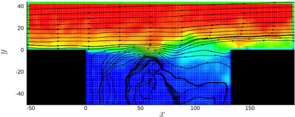
-50 0 50 100 150 -40 -20 0 20 40 x y
Figure 2.9: TR-PIV snapshot of the longitudinal component U and flow streamtraces. Dimensions of the axes are in mm. The origin is the left corner of the cavity.
because of the highly-defined time resolution. LaVision’s FlowMaster time-resolved PIV systems include Phantom V.12 digital high-speed camera with 6242 Hz frame rate at full resolution of 1280 × 800 pixel, dual cavity high-repetition rate solid state laser up to several 10 mJ per pulse and up to 20 kHz repetition rate. All components are fully controlled from the DaVis software and LaVision’s High Speed controller (HSC). The HSC enables an easy use of high speed systems with typically demanding trigger requirements like the synchronization of the external frequency of the device with the recording rate of the measurement system.
The camera field of view has been fixed at 244mm × 94mm, with a magnification rate of 5.45 px/mm, so that the mean displacement of a particle between two images is 8 pixel. The nominal longitudinal velocity considered for the entire campaign is U0 = 34m/s and,
as stated in the previous section, the cavity fundamental frequency is fc ∼ 125Hz. In
order to have a time resolution defined enough to permit the reconstruction of the cavity dynamics, we want to have at least 20 points per period, so the sampling frequency is fs = 3kHz (6kHz for single image). For each acquisition it is possible to store 7500
images, corresponding to about 60 periods.
Velocity field estimation has been realized through the software F OLKI-SPIV (Cham-pagnat et al., 2011). Particles’ displacement is computed by a correlation made on each pair of images divided in interrogation windows of 15 pixels. In Fig. 2.9 is shown a snap-shot acquired with the TR-PIV technique. The quality of the camera acquisition permits to appreciate the velocity fluctuations in the mixing layer. The oscillating behavior is clearly visible as well as the cavity recirculation on the bottom of the cavity, evidenced by velocity streamstraces.
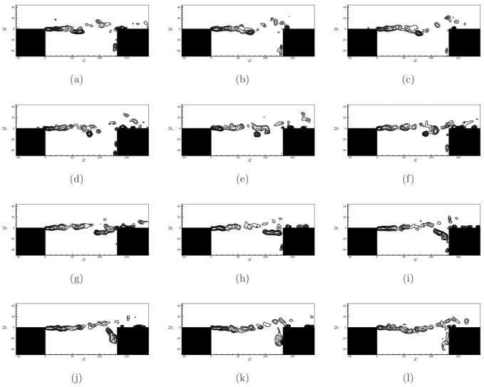
The high spatial and time resolution allows also to compute and observe the evolution of vortical structures. In Fig. 2.10, the vorticity component ωz is represented in a series
2.2. TIME-RESOLVED PIV 23 -50 0 50 100 150 -40 -20 0 20 40 x y (a) -50 0 50 100 150 -40 -20 0 20 40 x y (b) -50 0 50 100 150 -40 -20 0 20 40 x y (c) -50 0 50 100 150 -40 -20 0 20 40 x y (d) -50 0 50 100 150 -40 -20 0 20 40 x y (e) -50 0 50 100 150 -40 -20 0 20 40 x y (f) -50 0 50 100 150 -40 -20 0 20 40 x y (g) -50 0 50 100 150 -40 -20 0 20 40 x y (h) -50 0 50 100 150 -40 -20 0 20 40 x y (i) -50 0 50 100 150 -40 -20 0 20 40 x y (j) -50 0 50 100 150 -40 -20 0 20 40 x y (k) -50 0 50 100 150 -40 -20 0 20 40 x y (l)
Figure 2.10: Vorticity ωz development over a characteristic period.
cavity mixing layer can be followed through time by observing a particular structure formed at x = 50mm in Fig. 2.10(a). This eddy progressively detaches from the leading edge vorticity tounge (Fig. 2.10(b)-2.10(d)), regroups with smaller eddies (Fig. 2.10(e)-2.10(g)), impacts on the downstream wall (Fig. 2.10(h)-2.10(k)) and finally looses energy and dissolves (Fig. 2.10(l)). This cycle is representative of the quantity of time information obtained through the TR-PIV.
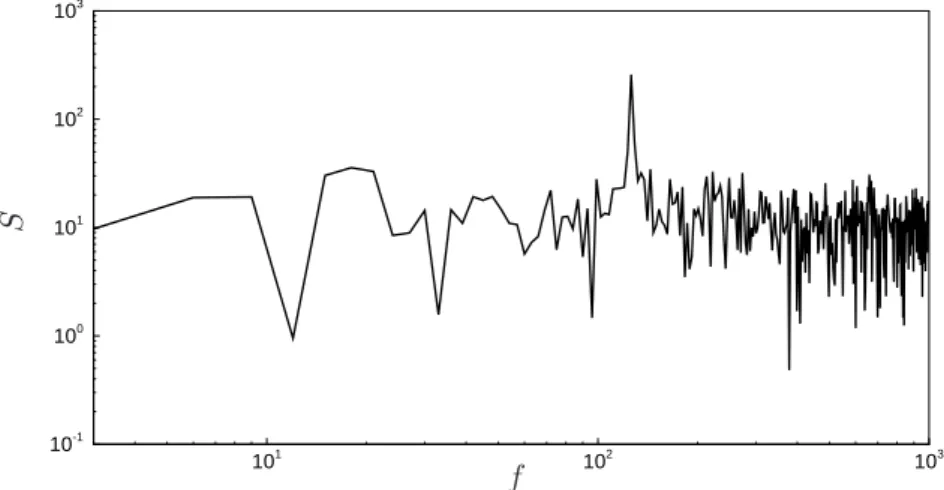
An important information obtained with the time resolution granted by TR-PIV mea-surements, is the frequency content. The acquisition capacity is limited to 16 Gb, cor-responding to about 8000 snapshots acquired at 3kHz. With this amount of data, it is possible to produce a power spectra as that pictured in Fig. 2.11. It is obtained from a single point measure over 4096 snapshots. We can observe two important features of the PIV acquisition: the presence of high-frequency noise and the characteristic peak at 126 Hz that confirms qualification results obtained with hot-wire probe and unsteady pressure sensors and represented in Fig. 2.3 and 2.7(b).
101 102 103 10-1 100 101 102 103 f S
Figure 2.11: Power spectra S of the velocity field computed from TR-PIV measurements. Frequencies are expressed in Hz.
Chapter 3
Non-linear model identification
This chapter describes the system-identification technique used to obtain a non-linear reduced model of a cavity flow. The interest of studying this approach stands in the possibility of application on closed-loop control of oscillating flows. The cavity flow char-acterized in the previous section is used to develop the necessary tools to obtain the reduce model. It consists on a oscillating flow with a well-defined peak at 126 Hz, but the dy-namics are strongly non-linear. This non-linearity has to be taken into account, since the reduced model is derived directly from experimental measurements.
This approach can lead to important results, but using experimental results, with noise and all the complexities coming from a real case, to identify a non-linear model is a path still not explored. The interest is then to understand the real potential of this technique, focusing on the meaning of each parameter and the consequences generated on the identification process.
As explained, measurements from experiments contain a number of information that can effect the identification. A treatment of these results has to be previewed, in order to simplify the identification of the most important dynamics, namely the first harmonic. The application of filters to real measurements has to consider that the main objective is the closed-loop control that implies real-time alteration of the flow. The effect of introducing delays into the system has to be analyzed carefully.
The chapter is structured as follows: non-linear reduced-order models are introduced in Sec. 3.1. A particular focus is given to those models obtained from Proper Orthogonal Decomposition, as Galerkin projection and system identification, to introduce how the structure of the model comes from the physics of the cavity flow. Sec. 3.2 treats routine to obtain POD modes and time projections that will be used as model regressors. Time-filtering on trajectories are discussed in this same section giving a critical comparison between original data and filtered ones. Last section (3.3) is devoted to the identification process and all those problems caused by non-linearity, time delay and time integration, pointing out the difficulty of this approach with a real non-linear case.
3.1
Non-linear reduced models
Methods of analysis and control of cavity flow oscillations rely on the knowledge of a model representing the most important dynamics of the system. As in many fluids problems, in cavity flows one does need to control only the main instabilities and larger eddies. A model reduction based on an energetic principle should be sufficient to successfully approximate the limit cycle of the cavity tones.
In this section, we then discuss non-linear reduced-order models based on Proper Or-thogonal Decomposition (POD). In particular, we focus on reduced model obtained by Galerkin projection of Navier-Stokes equations and on input/output system identification. Galerkin projection, due to its widespread use in closed-loop control, is taken as refer-ence for the algorithm structure design. However, the limitations and drawbacks of its requirements are used to motivate the choice of focusing on the system identification ap-proach to obtain the ROM. In particular, we highlight the advantages of the identification technique, which relies only on dynamics directly observed from measurements.
3.1.1
Proper orthogonal decomposition
The POD was introduced in turbulence by Lumley (1967) and is widely used to extract coherent structures existing in turbulent flows. It consists in finding a deterministic function Φ(x, y) that describes the spatial location of the most representative structures of the instance U(x, y, t). The time dependent quantity in our case stands for the velocity field U = (U, V ), acquired from the TR-PIV measurements.
The method used to compute POD, known as Snapshot method, has been introduced by Sirovich (1987). For a given set of M snapshots, it reduces to an eigenvalue problem
M
X
i=1
C(ti, tj)an(ti) = λnan(tj), (3.1)
with the correlation tensor C(ti, tj), defined through the inner product:
C(ti, tj) =
∆x∆y
4 [U
∗
iUj + Vi∗Vj] , (3.2)
where ∆x and ∆y represent the spatial discretization in the longitudinal and normal direction respectively. The solution of the eigenvalue problem gives M eigenvalues λn
(n = 1, ..., M ) and the associated eigenvectors φn. The eigenvalues, since the time instance
considered is the velocity field, represent the contribution of each mode to the total kinetic energy. By projecting each velocity component onto the normalized eigenvectors, following an energetic criteria that keeps only the most energetic N eigenvalues, the modes Φu
3.1. NON-LINEAR REDUCED MODELS 27
and Φv
n(x, y) can be easily computed as:
Φun(x, y) = √1
MU φnpλn, (3.3a)
Φvn(x, y) = √1
MV φnpλn. (3.3b)
The obtained functions represent a couple of normalized and bi-orthogonal basis, that is commonly used in model reduction.
The last step is then to compute the temporal projections an(t). For each mode the
nth trajectory is obtained by:
an(t) =
∆x∆y
4 (U
∗Φu
n+ V∗Φvn) . (3.4)
The velocity field can be approximated, with relatively good accuracy, with a small number of modes, due to the energetic efficacy of POD basis. This is the great advantage of a POD-based reduction, along with ease in solving an eigenvalue problem from an elevated number of snapshots.
3.1.2
Galerkin projection
The most classical and used model reduction technique in flow control is the Galerkin projection. It consists in projecting Navier-Stokes equations onto an orthogonal basis that energetically reproduces the main features and the input-output behavior of the original system. The choice of the basis is then crucial and can lead to undesired effects. It is typically used in numerical flow control applications, as we will do in Chapter 4, as well as in experimental environments. However, our purpose is not to analyze in detail such technique, but Galerkin projection is here considered for its wide use in flow control, to highlight its limitations and to introduce the resulting structure of the model, with particular focus on non-linear terms. For more details about this technique, the reader is referred to a number of references such as Rowley et al. (2004), Rowley and Batten (2008), Cordier et al. (2008), and Bergmann et al. (2009).
The reduced model is derived from Navier-Stokes equations. The velocity field can be approximated with the product of the POD functions Φn(x, y) with the time projections
an(t) related to the N most energetic eigenvalues λn, as:
U(x, y, t) ≈
N
X
n=1
Φn(x, y)an(t). (3.5)
problem becomes, in a general case, a problem for the time projections an(t): dan(t) dt = An+ N X i=1 Bnjai+ N X i=1 N X j=1 Cnijaiaj, n = 1, ..., N. (3.6)
where coefficients An, Bni and Cnij are constants, and N corresponds to the number of
modes used in the basis. Note that non-linear terms arise from the projection of the Navier-Stokes equations onto the POD basis. The same structure, will be used in the system identification process, considering only non-linear terms with a physical meaning. This method is widely used in a great number of applications. However, the reduced models based on Galerkin projection present some notable limitations and drawbacks. The model must accurately describe non-linear dynamics since time-integration could lead to a final state different from the initial assumption. Another problem is represented by the necessity of an observable basis, that implies an adjoint simulation. The spatial representation of the actuator represents a limit in experimental applications and an additional model is normally required. Noise has to be treated with particular accuracy and a statistical information is required for the Kalman filter estimation.
3.1.3
System identification
An alternative approach to obtain a reduced-order model is the system identification. The great advantage of this technique is that it only relies on data arising from simulations or experiments. The system is treated more as a black-box where the only interest is in the frequency response for a given set of known data.
As for Galerkin projection, for system identification technique, a reduction of the model is necessary to perform flow control. The choice of the same basis will lead to the same reduced-order model for a projected or an identified model. In this case, the structure in Eq. (3.6) can be used to identify coefficients from known data. This same structure can be modified by adding more terms if necessary, to improve the predicted output.
Independently from the used algorithm, the system identification technique consists in two different phases: a learning phase followed by a validation. In the first, coefficients are computed with a least-square method in order to fit a known set of data. In the second phase, the same coefficients are kept constant and the capacity of the model to reproduce a different data-set is validated. For this purpose, different parameters and features can influence the final result, as the number of previous known data, basis dimension, non-linearities.
Even though system identification techniques seem to be perfect for experimental applications, it presents some limitations that can be summarized in the following. The
3.2. POD FROM TR-PIV 29
main problem is the treatment of the non-linear dynamics. Dealing with non-linearity is a big challenge since previous positive results are obtained on linear or linearized dynamics and the behavior in a case such as that of the S19 cavity flow is still unknown. In addition, we have to consider that the regression algorithm has to be tuned. Coefficients are usually based on a physical interpretation and setting them properly requires some attention.
3.2
POD modes from TR-PIV measurements
The basis chosen for model reduction is obtained from POD modes, that were obtained by processing TR-PIV acquisitions. In this section the procedure to obtain POD and time trajectories is described. The objective is to have time-evolving projection coefficients that can be used in the system identification procedure. Time filtering will be used to focus on the low-frequency dynamics of the cavity flow.
3.2.1
POD modes and trajectories
The computation of POD modes and projections can be easily achieved from TR-PIV measurements. The series of snapshots acquired in the experimental campaign is divided into different velocities and configurations. For this study, an unperturbed configuration at the nominal velocity of 34 m/s has been chosen to design the reduced-order model.
In order to compute the correlation term in Eq. (3.2), 500 snapshots, corresponding to about 20 periods, are assembled as Np× Ns matrix, where Np is the number of geometric
points, equal to 6400, and Nsis the number of snapshots. The geometric parameters used
to non-dimensionalize the modes are ∆x = ∆y = 1.92mm.
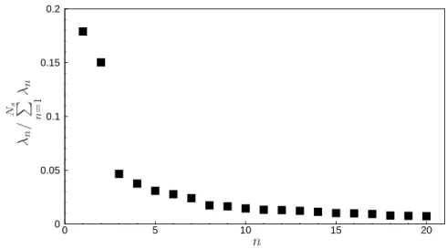
The solution of the eigenvalue problem leads to the eigenvalues represented in Fig. 3.1. It is evident that the first two modes represent the biggest amount of energy, though lower than the 40% of the total. In order to have a representation of at least 50% of the total energy, we need to consider the first 9 modes ; note that considering more POD modes will increase the number of regressors in the system identification process. A steeper slope in the eigenvalues contribution would be preferred for model reduction and a way to decrease the importance of less energetic modes has to be found.
POD modes Φu
n and Φvn are computed from Eq. (3.3). In Fig. 3.2 are represented the
first 2, the 4th and the 5th POD modes. The spatial distribution of the POD structures
highlights the coupling of each pair of modes, as expected. The same expectation resided in the smaller dimension of eddies for less energetic modes. These results are then coherent with all the previous studies on cavity flows.
The spatial distribution corresponding to the third mode is unexpected, since it shows a strong asymmetry in the longitudinal component (Φu
3) and a very weak intensity in
the normal component (Φv
0 5 10 15 20 0 0.05 0.1 0.15 0.2 n λn / NsP n= 1 λn
Figure 3.1: Contribution of the first 20 eigenvalues computed from the correlation term corresponding to a set of Ns =500 snapshot acquired at 3 kHz with a flow at 34 m/s.
linked more to the mean flow than to fluctuations, but it turns out that it is a spurious mode. By a detailed observation of velocity fields, we noticed that its presence is produced by reflections generated by the laser sheet which were not completely eliminated. The energetic level is huge in the longitudinal direction and very low in the vertical component. This is caused by the presence of a reflection in the downstream corner of the cavity that influences the velocity field in that region. The result is a discontinuity in the flow direction and consequently a high level of energy. Since this mode does not represent any physical turbulent eddy, we choose not to consider it as part of the basis for model reduction.
The last step is to compute projections an(t) that will be used as regressors in the
system identification process. From Fig. 3.4 we can observe the time behavior of the first four trajectories, i.e. the projections of the snapshots onto the POD basis, within the first 25 periods. As expected from POD modes, a1 and a2 are more regular and more
intense than the followers since snapshots are projected to symmetric modes as those in Fig. 3.2(a)-3.2(d). The characteristic frequency is evident in all cases, thanks to the time resolution of 20 point per period. However, even in projections related to the most energetic modes, a modulation is present indicating the presence of several frequencies around the peak at 126 Hz. By observing the smallest projections, a high frequency noise is also remarked. For these reasons an analysis of snapshot filtering seems an interesting contribution.
3.2.2
Time-filtering
The observation of time projections leads us to filter TR-PIV measurements in order to avoid high-frequency noise and modulations around the characteristic peak. This pro-cedure is not common in experimental results, but since the objective is to develop an