Uncertainty quantification in system-level prognostics: application to Tennessee Eastman process

OATAO is an open access repository that collects the work of Toulouse

researchers and makes it freely available over the web where possible

Any correspondence concerning this service should be sent

to the repository administrator:

tech-oatao@listes-diff.inp-toulouse.fr

This is an author’s version published in: http://oatao.univ-toulouse.fr/23821

To cite this version:

Tamssaouet, Ferhat

and Nguyen, Thi Phuong Khanh

and

Medjaher, Kamal

and Orchard, Marcos E. Uncertainty

quantification in system-level prognostics: application to Tennessee

Eastman process. (2019) In: The sixth (6th) edition in the series of

the International Conference on Control, Decision and Information

Technologies - CODIT 2019, 23 April 2019 - 26 April 2019 (Paris,

France).

Uncertainty Quantification in System-level Prognostics: Application to

Tennessee Eastman Process

Ferhat Tamssaouet1, TP Khanh Nguyen1, Kamal Medjaher1 and Marcos E. Orchard2

Abstract— This paper addresses the problem of uncertainty quantification in system-level prognostics. To this purpose, a three-step methodology, based on the inoperability input-output model, is presented. The first step concerns the estimation of the system inoperability, using a new adapted particle filtering method, while considering the interactions between its components. The second step focuses on the long-term prediction of the system inoperability in order to determine its evolution. Finally, in the third step, a method for calculating the remaining useful life of the system, based on the system configuration, is formulated. The proposed methodology is applied on data obtained from the Tennessee Eastman Process simulations to predict the shutdown due to violation of process constraints.

I. INTRODUCTION

Prognostics and Health Management (PHM) is essential to ensure safe, reliable and correct operation of complex technical systems. Among the key elements of PHM, prog-nostics allows predicting the remaining useful life (RUL) of components, subsystems or systems before they become inoperable. Based on these predictions, effective actions can be taken to minimize losses, optimize maintenance, and extend components life.

According to practical requirements, prognostics received a great attention in literature. However, it has often been approached from a component view without considering interactions with other system components and the environ-ment [1], [2]. Hence, for complex engineering systems, it is necessary to study the concept of failure prognostics at system-level by considering the mutual interactions between its elements.

Moreover, notwithstanding the increasing accuracy and precision of prognostics algorithms, their objects of study, i.e. degradation and failure mechanisms, remain stochastic phenomena and, therefore, the uncertainty cannot be elimi-nated totally [3]. Indeed, various sources contribute to make the estimation and prediction of one system state uncertain. The number of the uncertainty sources will rapidly increase when considering prognostics at system-level.

To provide a solution to the problems stated above, a new method that allows quantifying the uncertainty in the system remaining useful life (SRUL) prediction is proposed in this paper. It introduces, as a first contribution, a novel system-level prognostics framework based on the inoperability input-output model (IIM). This model allows tackling the issue

1_{F. Tamssaouet, TPK Nguyen and K. Medjaher are with Laboratoire} G´enie de Production, LGP, Universit´e de Toulouse, INPT-ENIT, Tarbes, Franceferhat.tamssaouet@enit.fr

2_{M. Orchard is with the department of Electrical Engineering, University} of Chile, Santiago, 8370451, Chile.

related to the interactions between the system components. As a second contribution, a methodology to quantify uncer-tainty in the SRUL predictions based on the particle filtering is proposed. This methodology will be applied to the well-known Tennessee Eastman Process (TEP) to demonstrate its effectiveness.

The remainder of the paper is organized as follows. Section II presents the new system degradation model which is based on the inoperability input-output model. Section III describes the proposed methodology for uncertainty quantifi-cation and the SRUL determination. Section IV deals with uncertainty modeling and quantification for the Tennessee Eastman Process. A comparison of the obtained results with process real data, were made in order to show the effectiveness of the proposed method. Finally, Section V concludes the paper and gives some future works.

II. INOPERABILITYINPUT-OUTPUTMODEL

One of the main challenges for the SRUL prediction is to develop a model that allows taking into account the mutual components interactions and effects of the mission profile on the degradation evolution. For this purpose, a new model for the degradation of multi-component systems is proposed in this section, that is based on the inoperability input-output model (IIM). The proposed model is then used in Section III to quantify the uncertainty when predicting the SRUL.

The proposed model is inspired by the IIM which is an extension of the input-output model developed by Leontief Wassily in 1936 [4]. The IIM model and its variants are usually used to investigate the global effects of negative events on highly interdependent infrastructures or multi-sector economies [5], [6]. This is achieved by using the concept of inoperability, which is defined as the inability of a system to perform its intended functions. The aptitude of the IIM to consider mutual interactions between numerous elements offers a promising perspectives when applying it in PHM domain.

The IIM adapted to prognostics is proposed firt in [7] and is represented by the following formula:

q(t) = K(t).[A.q(t − 1) + c(t)] (1) where:

• q(t) is a vector representing the overall inoperability of the system components at time t. Each component of this vector is a value between 0 and 1, where qi(t) =

0 corresponds to a healthy component (with an ideal performance) and qi(t) = 1 to a faulty component (no

• A is a matrix representing the interdependencies be-tween the system components. Each element ai j of the

matrix corresponds to the influence of the inoperability of component j on the inoperability of component i. The bigger ai j is, the greater is the influence of j on i. • c(t) is a vector representing the internal inoperabilities of the system components at time t, i.e. the degradation of the component due to wear, corrosion or any other failure mechanism. The parameter ci(t) can be obtained

by normalizing the health indicator of component i to its failure threshold.

More details about the normalization of the component’s health indicator can be found in [7].

• A.q(t) represents the inoperability of a component due to its interdependencies. This quantity informs about the degradations caused by the interactions between components.

• K(t) is a diagonal matrix representing the factors in-fluencing the inoperabilities of components at time t with respect to the system inputs (mission profiles and environment conditions). Each element ki is specific to

only one component i.

As one can notice in (1), the degradation of component

i, characterized by an inoperability qi(t), depends on its

inherent natural degradation mechanisms expressed by ci(t)

and the degradation induced by the interactions with other components through the term A.q(t). By integrating these two types of degradation, IIM can estimate the health state of systems more accurately.

The advantages of using the IIM to model systems are multiple, among which: 1) the normalization of health in-dicators to obtain inoperability allows modeling systems with heterogeneous components (different health indicators, range values, degradation patterns and failure thresholds); 2) IIM describes a direct relationship between the mission profile effects and the degradation evolution, which eases the adaptation of the mission profile to extend the system life; 3) multiplying the inoperability by 100 gives a percentage of the component degradation relative to its failure threshold, which facilitates communication with the decision-makers.

III. UNCERTAINTYQUANTIFICATION INSYSTEM-LEVEL

PROGNOSTICS

The methodology proposed in this paper, and illustrated by Fig. 1, combines the estimated and the predicted system inoperabilities to compute the SRUL. The computational process requires the component-level degradation models, the interactions between the components, the thresholds related to each failure mode and the distributions associated to the uncertainties. The details of the three main steps of the proposed methodology is explained in the next subsections.

A. Inoperability uncertainty estimation

The objective of the first step of the methodology is to estimate the inoperability posterior density of the M system components at each time instant k given the observations

yk. To do that, the particle filtering, which is a popular

Fig. 1: Uncertainty quantification methodology for system-level prognostics.

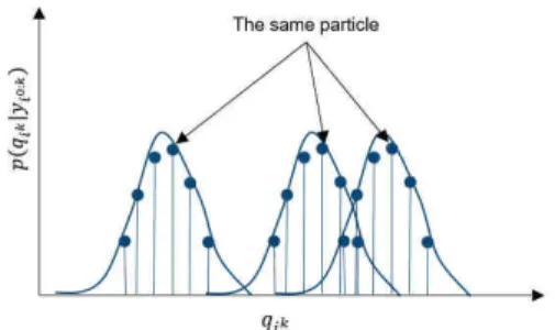
technique explored by several works in prognostics domain [8], [9], is used. This tool can be applied to systems with non-linear dynamics and non-Gaussian noise. However, contrary to traditional utilization, in this paper a particle is considered as a vector representing the state of health (inoperability) of the system components. Thus, the weight associated to a particle represents the approximation of the inoperability probabilities of all the M components at the same time, as shown in Fig. 2. The process of estimating the inoperability state of a system at time k is explained below.

Firstly, using the IIM presented in Section II, the prior probability density distributions PDFs of the system compo-nents inoperabilities p(qk|qk−1) at time k are predicted based

on the ones at the previous time k− 1:

p(qk|qk−1) ∼ IIM(qk−1) (2)

Next, given new observations yk

i at time k for a component

i, i∈ {0, 1, ..., M}, the system posterior PDFs inoperabilities are updated by the particle filtering. In detail, considering a set of N particles{q(l)}l=1,...,N, their associated normalized

weights {w(l)_}

l=1,...,N are evaluated by the likelihood

func-tions p(yk

i|qki) using the importance distribution functions

π(qk i|qk−1i ,y1:ki ): w(l)_k ∝ w(l)_k−1 M

∏

process is applied in each time step to replace particles having low importance weights with particles that have higher importance weights.

The posterior PDFs of the system inoperability at time k (Fig. 1) can be approximated before the resampling step by:

p(qk|y0:k) ≈ N

∑

w(l)_k δq(l)k(qk) (4)

whereδ(·) denotes the Dirac delta function.

The estimation procedure is repeated at every instant k, k∈ {1, 2, ..., kp}, where kp is the starting time of the prediction

step presented in the next subsection.

B. Inoperability uncertainty prediction

Prognostics, and thus generation of long-term predictions, is a problem that goes beyond the scope of filtering problem, since it involves future time horizons in which no mea-surements are available for the Bayesian updating through the equation (3). Thus, the particle filtering, which is more suitable for estimation problems, needs to be adapted to use it for predictions.

In this work, to reduce the computation requirement, we suggest to follow the procedure proposed in [10] and which is based on the assumption that the particle weights are constant from time kp to time k. According to this

procedure, the predicted PDF of the inoperability of the system’s components at time k (i.e., p(qk|y1:kp)) can be

obtained by applying recursively (2) to q(l)_k

p.

Once the prediction of the future system inoperability is done, it will be used to determine the system remaining useful life (SRUL), as explained in the next subsection.

C. SRUL determination

The SRUL provides information related to the time when the whole system fails (i.e., when the combined failures of individual components lead to system failure) [2] or when a system reaches performance level that is considered unacceptable. However, the consequence of the degradation of one or more components depends on the considered architecture (e.g. parallel or series). Therefore, the SRUL must be calculated according to system configuration.

Assuming that the system is healthy at time kp− th,

moment when the prediction algorithm is launched, the SRUL can be computed as follows:

SRU L= τF− kp (5)

with τF is the system time-of-failure ToF (or the system

end-of-life (EOL)). ToF is chosen in this work because it is a more general concept which can be used in multiple applications [11].

τF= in f (k ∈ N : system f ailure at k) (6)

In practice, and given the complexity of industrial systems, it is important to consider the uncertainty associated with the ToF. To do this, the notations and the new paradigms proposed in [8], [11] are used in the remainder of this paper.

Let’s denote a healthy system (with no occurrence of catastrophic failure) and a faulty system (with occurrence of catastrophic failure) at k− th by Hk and Fk, respectively.

Let’s also consider Hkp:k = (Hkp,Hkp+ 1, · · · , Hk) as the

sample space that determines all possible sequences where a system has not catastrophically failed until the time k. Then, according to the definition of the conditional probability, the failure probability at k− th is given by:

P(Fk) =

P(Fk,Hkp:k−1)

P(Hkp:k−1|Fk)

(7) As the system can only fail once (without maintenance), given that the failure has occurred at time k, the probability of staying healthy until time k− 1 is P(Hkp:k−1|Fk) = 1.

P(Fk) = P(Fk,Hkp:k−1) = P(Fk|Hkp:k−1)p(Hkp:k−1); ∀k > kp

(8) where P(Fk|Hkp:k−1) is given by:

P(Fk|Hkp:k−1) =

Z

Rnq

p( f ailure|qk)p(qk|y1:kp)dqk (9)

The second term of (8), p(Hkp:k−1), stands for the

prob-ability that one component is healthy from kp-th until time

(k − 1) − th, which can be expressed as:

p(Hkp:k−1) =

k−1

∏

p(Hh|hkp:h−1) (10)

As Fk and Hk are exclusive events, the failure event

can be modeled through a Bernoulli stochastic process:

p(Hj|Hkp: j−1) = 1 − p(Fj|Hkp: j−1). It follows that: p(Hkp: j−1) = k−1

∏

The expressions presented in (8) and (11) are valid whether for prognostics of a single component or complex systems. However, when considering a multi-components system, the way of characterizing p(Fk|Hkp:k−1) will change

according to the system configuration.

For exemple, in series configuration of M components, the probability that a system will fail at time k, conditional that it is healthy at k− 1, is a finite union of the components failure events. As only one component failure can appear at an instantaneous moment, the components failure events can be considered as incompatible. Then, the system failure probability can be written as:

p(Fk|Hkp:k−1) = M

∑

ik|Hkp:k−1) is the probability that component i will

fail at time k, conditional that the system is healthy at k− 1. Then: p(Fk|Hkp:k−1) = M

∑

Fig. 3: P&ID of the Tennessee Eastman Process [12].

IV. TENNESSEEEASTMANPROCESS

In this section, the proposed methodology is applied to solve the failure prognostics issue of the Tennessee Eastman Process (TEP).

A. Process description

The Tennessee Eastman Process built by Eastman Chemi-cal Company has been widely used as a realistic benchmark for process control optimization, fault diagnostics and, to a lesser extent, for component-level prognostics. Downs and Vogel [12] described it in detail and provided its simulation where the components, kinetics, and operating conditions have been modified for proprietary reasons. The TEP in-volves five major units (working in open-loop) including a two-phase reactor, a partial condenser, a separator, a stripper, and a compressor. The schematic piping and instrumentation diagram (P&ID) of the TEP is shown in Fig. 3.

In the TEP, the gaseous reactants{A,C, D, E} are fed to the reactor where the liquid products{G, H} and the byproduct {F} are formed through the following exothermic reactions:

         A(g) +C(g) + D(g) → G(l), A(g) +C(g) + E(g) → H(l), A(g) + E(g) → F(l), 3D(g) → 2F(g).

The process has a total of 53 measured variables, of which 22 variables are continuous process measurements (such as: temperatures, pressures, flow rates, levels), 19 variables are composition measurements and remaining 12 are manipulated variables. 28 faults can be injected in the process [13], which can be related to step changes, drifts, and random variation of variables, etc.

B. Problem Statement

In this case study, we consider a failure as interruption of the operational continuity resulting from violation of the variables shutdown limits. Therefore, only components with shutdown constraints are considered, i.e. reactor, stripper

and separator. Each of these components is monitored by a single parameter: pressure for the reactor, and level for the stripper and the separator. Table I lists the specific operational constraints related to the system parameters that the control system should respect.

TABLE I: Process operating constraints [12].

Normal operating limits Shut down limits Process variables Low limit High limit Low limit High limit

Reactor pressure none 2895 kPa none 3000 kPa

Separator level 3.3 m 9.0 m 1.0 m 12 m

Stripper level 3.5 m 6.6 m 1.0 m 8.0 m

In Matlab R _{simulations of the TEP [14], three}

distur-bances predefined in [13] were injected. Two disturdistur-bances are deviations in the reactor and the stripper parameters that are, respectively: deviation in the reactor cooling water flow (c1(t)) and deviation in the heat transfer of the heat

exchanger of the stripper (c2(t)). These deviations c1(t)

and c2(t) are assumed to follow equations (14) and (15),

respectively.

c1(t) = α.c1(t − 1) + β (14) c2(t) = γ.c2(t − 1) (15)

withα, β and γ are the parameter of the two models. As shown in Fig. 4, when these two faults are injected, the system shuts down at 0.8 hour.

The third injected fault is a random variation of the reactor cooling water inlet temperature and can be considered as process noise.

The purpose, here, is to estimate the SRUL when taking into account the process uncertainty, which is characterized by a random variation of the reactor cooling water inlet temperature. To do this, the proposed IIM, Eq.(1) where c(t) is given by Eq.(14) and (15), is used to model the system degradation. The IIM parameters are estimated and adjusted thanks to data collected from the TEP simulation. In the next subsection, construction of the IIM is detailed.

C. Inoperability input-output model of TEP

The raw data acquired from the TEP simulation are normalized to the initial state and the failure threshold, as

Fig. 4: Components inoperabilities evolution when consider-ing two faults.

shown in Fig. 4. They represent the inoperability of the three components: reactor q1(t), stripper q2(t) and separator q3(t).

Their initial states correspond to the parameters base value [12] and the failure thresholds to the shutdown limits values (Table I).

The IIM of the TEP is built from data obtained after injection of these faults. It should be noted here that the IIM model does not model the physical phenomena operating in the process, but is more used to fit the actual data of the process. For this case study, the interdependence matrix (A) is estimated and adjusted to make the proposed model better fit the process data. Then, we obtain the following result:

A=   0 0.1 0 10−5 0 0 0.4 0.3 0   (16)

Regarding the matrix K, it has been assumed that the environmental conditions have no effects on the evolution of the components inoperabilities. Therefore, its diagonal is equal to 1.

D. Inoperability estimation and prediction

After application of the random variation of the reactor cooling water inlet temperature, the data obtained from the process and the built IIM are used in the particle filtering to estimate the components inoperabilities. To evaluate the in-operabilities densities, 200 particles were used with the initial distributions of the components inoperabilities considered as Gaussian. The selection of the particles to be retained after each filtering step was done by using residual resampling.

When the inoperability of one component exceeds the nor-mal operating limits (as indicated in Table I), the prediction

step will be launched (at time kp).

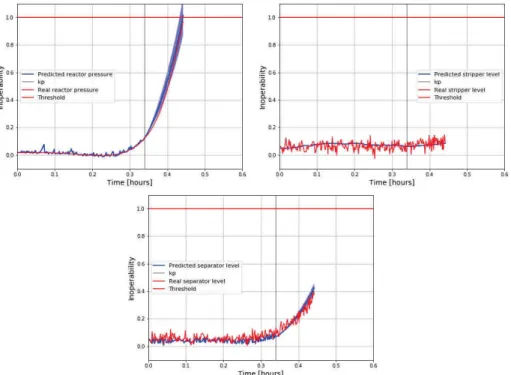
The results of the estimation and prediction of the inoper-abilities uncertainty of the system components are shown in Fig. 5. The reactor is the first component to go out of its normal operating limits after 0.34 hour. This time corresponds to the time where the long-term inoperability prediction is launched. Also, it is the reactor pressure, that triggers the system shutdown (system failure) at 0.44 hour.

From these results, we can highlight the power of estima-tion and predicestima-tion of the proposed methodology. Indeed, before the adding of the random variation (the process noise), the system shuts down at 0.8 hour and after the fault injection, it shuts down at 0.44 hour. Despite this high process variability, the particle filtering was able to estimate the actual inoperability of the system (as shown in Fig. 5). Also, one can notice that the uncertainty related to the predicted inoperability increases for k > kp. This is due to the

fact that no measurements were received and, therefore, there is neither updating of the particle weights nor resampling.

E. SRUL determination

For this case study, the operability of the studied system depends on the operability of its components since they all contribute to realization of the system function (G and H production). Therefore, one can conclude that the system has a series architecture. Consequently, the system ToF probability will be determined using the equation (13).

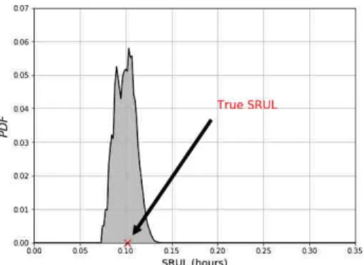
Fig. 6 shows the PMF of the SRUL. The mean value of the SRUL is equal to 0.1 hour. The true SRUL, which is equal to 0.102 hour, is within the 95% confidence interval of the predicted SRUL distribution. We can conclude that

Fig. 6: SRUL probability distribution of the system.

the predicted SRUL is close to reality and is slightly pes-simistic, which does not put the system, its operators and the environment in danger.

In order to discuss the results of the proposed method-ology, a study of the impact of the prognostics horizon on uncertainty intervals is performed by considering the α-accuracy metric, which determines whether a prediction falls within anα% interval. In fact, α-accuracy is a useful metric to judge if one prognostics algorithm converges to the true value as more information are accumulated over time. Indeed, a faster convergence is desired to achieve a high confidence, keeping the prediction horizon as large as possible. To that end, in this study, the prognostics time has been varied within the interval shown in Fig. 7 and the accuracy is defined with α= 10%. The figure shows the mean values and uncertainties of the predicted SRUL distributions compared with the true SRUL. As it can be seen, the prediction of the SRUL becomes more accurate each time the measurements are obtained. One can also notice that for t≤ 0.6, the SRUL remains almost constant because the values of the monitored parameters do not change a lot, as it can be seen in Fig. 4.

V. CONCLUSION

A methodology for the uncertainty quantification at system-level prognostics is proposed in this paper. This methodology results in three main contributions. The first concerns the modeling of the system degradation by using the

Fig. 7: SRUL prediction performance with α= 0.1.

inoperability input-output model. The second deals with the health state estimation based on an adapted particle filtering. Finally, the third contribution is related to the calculation of the system remaining useful life, based on the recent developments and achievements proposed at component-level prognostics and generalized in this paper to system-level prognostics.

The proposed methodology was applied on the Tennessee Eastman process in order to predict the shutdown time caused by violation of the process constraints. The obtained results show the effectiveness of the methodology in estimating and predicting the system remaining useful life and characteriza-tion of uncertainty.

For future work, a systematic method to determine the IIM parameters from a real data will be proposed. Also, it would be worthwhile to apply the other predefined disturbances in the TEP in order to test the robustness of the methodology.

REFERENCES

[1] V. Atamuradov, K. Medjaher, P. Dersin, B. Lamoureux, and N. Zerhouni, “Prognostics and health management for maintenance practitioners-review, implementation and tools evaluation,”

Interna-tional Journal of Prognostics and Health Management, vol. 8, no. 060, pp. 1–31, 2017.

[2] L. R. Rodrigues, “Remaining useful life prediction for multiple-component systems based on a system-level performance indicator,”

IEEE/ASME Transactions on Mechatronics, vol. 23, no. 1, pp. 141– 150, 2018.

[3] B. Saha and K. Goebel, “Uncertainty management for diagnostics and prognostics of batteries using bayesian techniques,” in Aerospace

Conference, 2008 IEEE. IEEE, 2008, pp. 1–8.

[4] W. W. Leontief, “Quantitative input and output relations in the eco-nomic systems of the united states,” The review of ecoeco-nomic statistics, pp. 105–125, 1936.

[5] Y. Y. Haimes and P. Jiang, “Leontief-based model of risk in com-plex interconnected infrastructures,” Journal of Infrastructure systems, vol. 7, no. 1, pp. 1–12, 2001.

[6] J. R. Santos and Y. Y. Haimes, “Modeling the demand reduction input-output (i-o) inoperability due to terrorism of interconnected infrastructures,” Risk Analysis: An International Journal, vol. 24, no. 6, pp. 1437–1451, 2004.

[7] F. Tamssaouet, T. P. K. Nguyen, and K. Medjaher, “System-level prognostics based on inoperability input-output model,” in Annual

conference of the prognostics and health management society, vol. 10, 2018.

[8] D. E. Acu˜na and M. E. Orchard, “Particle-filtering-based failure prognosis via sigma-points: Application to lithium-ion battery state-of-charge monitoring,” Mechanical Systems and Signal Processing, vol. 85, pp. 827 – 848, 2017.

[9] M. Orchard, “A particle filtering-based framework for on-line fault diagnosis and failure prognosis,” Ph.D. dissertation, Georgia Institute of Technology, Atlanta, CA, 2006.

[10] A. Doucet, S. Godsill, and C. Andrieu, “On sequential monte carlo sampling methods for bayesian filtering,” Statistics and computing, vol. 10, no. 3, pp. 197–208, 2000.

[11] D. Acu˜na and M. Orchard, “A theoretically rigorous approach to failure prognosis,” in Annual conference of the prognostics and health

management society, vol. 10, 2018.

[12] J. J. Downs and E. F. Vogel, “A plant-wide industrial process control problem,” Computers & chemical engineering, vol. 17, no. 3, pp. 245– 255, 1993.

[13] A. Bathelt, N. L. Ricker, and M. Jelali, “Revision of the tennessee eastman process model,” IFAC-PapersOnLine, vol. 48, no. 8, pp. 309– 314, 2015.

[14] N. L. Ricker, “Tennessee eastman challenge archive,” http://depts.washington.edu/control/LARRY/TE/download.html, online; accessed 15 December 2018.