OATAO is an open access repository that collects the work of Toulouse
researchers and makes it freely available over the web where possible
Any correspondence concerning this service should be sent
to the repository administrator: [email protected]
This is a publisher’s version published in: http://oatao.univ-toulouse.fr/23395
To cite this version:
Romdhane, Hela and Soualmia, Amel and Cassan, Ludovic
and Dartus, Denis Flow over flexible vegetated bed :
evaluation of analytical models. Journal of Applied Fluid
Mechanics, 12 (2). 351-359. ISSN 1735-3572
Official URL:
https://doi.org/10.29252/jafm.12.02.29463
Journal of Applied Fluid Mechanics, Vol. 12, No. 2, pp. 351-359, 2019. Available online at www.jafmonline net, ISSN 1735-3572, EISSN 1735-3645. DOI: 10.29252/jafm.12.02.29463
Flow over Flexible Vegetated Bed: Evaluation of
Analytical Models
H. Romdhane
1, A. Soualmia
1,
L. Cassan
2†and D. Dartus
21National Agronomic Institute of Tunisia, University of Carthage, EL Menzah, Tunis, 1002, Tunisia
2 Fluid Mechanics Institute of Toulouse, INP Toulouse, Toulouse, 31400, France
†Corresponding Author Email: [email protected] (Received July 27, 2017; accepted September 13, 2018)
A
BSTRACTThe development of vegetation in the river bed and in the banks can affect the hydrodynamic conditions and the flow behavior of a watercourse. This can increase the risk of flooding and sediment transport. Therefore, it is important to develop analytical approaches to predict the resistance caused by vegetation and model its effect on the flow. This is the objective of this work which investigates the ability of different analytical models to predict the vertical velocity profile as well as the resistance induced by flexible submerged vegetation in open channels. Then it is possible to select the appropriate model that will be applied in the real case of rivers. The model validation is determined after a comparison between the data measured in the different experiments carried out and those from literature. For dense vegetation, the role of the Reynolds number is emphasized in particular with a model using the Darcy-Brinkman equation in the canopy. With a simple permeability, this model is relevant to estimate friction. However, for larger Reynolds number, models based on the fully turbulent flow assumption provide better results.
Keywords: Analytical models; Experiments; Flexible vegetation; Open channel; Roughness.
1. INTRODUCTION
Vegetation in rivers and floodplains occurs in different forms; it can be flexible or rigid and submerged or emerged in the flows. It plays an important role in the flow patterns of many streams and rivers and can increase the risk of flooding. In fact, understanding vegetation flows is necessary to control flooding and the river ecosystem (Wu and He, 2009; Liu and Shen, 2008). The influence of vegetation on the water routing during flash flood events are also crucial because they are determinant for forecasting and alert (Douinot et al., 2017). Indeed, the double averaged approach (Nikora et al. 2001) used to study flow above vegetation is particularly adapted for routing process where vegetation is dense, when steep slopes involve uniform flow and with a weak submergence. In the last decade, much research has been devoted to understanding vegetation flow characteristics using laboratory experiments with natural or artificial vegetation (Poggi et al., 2004; Ghisalberti and Nepf, 2006; Le Bouteiller and Venditti, 2015). In fact, most of the developed relationships have adopted a two-layer approach. This method is based on dividing the flow domain into two-layer (Klopstra et al., 1997; Defina and Bixio, 2005;
Murphy and Nepf, 2007).
The first layer through the vegetation is called” vegetation or canopy layer”, the second layer above is called” upper layer”. The logarithmic flow velocity profile is adopted to solve the velocity above the vegetation, and the equation of momentum in the vegetated layer.
For non-vegetated flow, the vertical distribution of velocity is directly related to the shear stress of the bed, whereas for a vegetated flow, it is linked to the vegetation drag because the roughness of the vegetation is much greater than the roughness of the riverbed. Here, this study compares different analytical models based on the two-layers approach to analyze their performances. We focus on models which can predict the vertical flow velocity profiles through the submerged flexible vegetation. In
Cassan et al. (2017), the computation of the velocity profile allows calculating the discharge for a large range of flow over rigid macro-roughness. The results have shown a quite good applicability for steep flow over gravels and rocks. For flexible canopy, the physical process could be different (monami wave, interaction stem-flow, stem vibration) (Marjoribanks et al., 2017; Kucukali and Hassinger, 2018) and it is proposed to assess the same methodology to obtain discharge. In previous studies Morri et al. (2015) and Katul et al. (2011)
have already compared the flow resistance provided by models where only one averaged velocity is
H. Romdhane et al. / JAFM, Vol. 12, No. 2, pp. 351-359, 2019.
352 given for each layer. Then we choose to evaluate the Huthoff model which seems to be the most pertinent for flexible vegetation (Morri et al., 2015) and three models using the double averaged approach (Nikora et al., 2001).
A model which provides the velocity distribution can appear more complex, but it can be used to understand pertinent phenomena involved in the hydraulic resistance (King et al., 2012) and transport phenomena. The models are compared for experiments from literature with flexible vegetation. Several studies had been already used (Poggi et al. 2009; Katul et al. 2011; Cassan and Laurens 2016), but we added to them more recent measurements (Le Bouteiller and Venditti, 2015).
Moreover, additional experiments were carried out in the case of dense canopy. These specific conditions were tested in order to understand difference between models based on Darcy-Brinkman equation (Rubol et al., 2018) and those with a turbulent drag force (Klopstra et al. 1997;
Meijer and Velzen 1999; Cassan and Laurens 2016).
2. MATERIALS AND METHODS The analytical and semi-analytical models evaluated in the paper are here presented. They consider a momentum balance in a uniform flow and vegetation. The vegetation is an arrangement of obstacle on which is applied a drag force. An additional stress is added representing the turbulent term in the flow or/and in the bed boundary layer (Huthoff et al., 2007). The drag force is expressed with a drag coefficient Cd and the frontal area by
unit width a (m−1). The frontal area can be obtained
with the number of stem per square meter, m, and the stem diameter D which are usually given. Except the Huthoff model, the Meijjer, Cassan and Rubol models are based on spatial and temporal averaged concept (Nikora et al., 2001), and the double averaged velocity at a given vertical position is denoted u. The deflected height stem is denoted
hp and the total water depth H. As consequence the
momentum balance in the upper layer leads to define the shear velocity as 𝑢∗= √𝑔𝑆(𝐻 − ℎ𝑝)
where g is the gravitational constant (9.81 m2/s) and S the friction slope which is equal to the bed slope
in the experiments considered. Above vegetation, a logarithmic profile is often assumed for velocity distribution (Klopstra et al. 1997; Defina and Bixio 2005; Meijer and Velzen 1999) (Eq. (1)).
𝑢 𝑢∗= 1 𝑘𝑙𝑛( 𝑧−𝑑 𝑧0) (1) where κ is the von Karman constant, d is the distance between the top of the vegetation and the virtual bed of surface layer, z0 is the height of the
roughness.
2.1. Huthoff et al., 2007
To determine the expression of velocity, Huthoff et al. (2007) applied the two-layer approach, and the flow into and out of vegetation is treated separately.
The averaged velocity within the vegetation layer
Ur is obtained by solving the momentum balance
and by the Strikler law for friction on bed (Eq. (2)). 𝑈𝑟= √1+ 2𝑔𝑆𝑏𝑏 32ℎ𝑝( 𝑘𝑠 𝐻)1/3 √ℎ𝐻 𝑝 (2) where b = 1/Cd m D is a drag length and m is the
number of stems per unit area.
In the upper layer, Huthoff et al. (2007) used the Boussinesq hypothesis to describe shear stress, and considered the dissipation at the top of the canopy. It is possible to scale the velocity above the canopy as a function of a turbulent length scale (Eq. (3)). By comparison with other possible length scales, the chosen value of l is given by the distance between stem s. Finally, in the upper layer, the averaged velocity expression is given by the following equation (Eq. (3)):
𝑈𝑠= 𝑈𝑟√ ℎ𝑝 𝐻( 𝐻−ℎ𝑝 𝑠 ) 2/3(1−(𝐻 ℎ𝑝) −5 ) (3) 2.2. Rubol et al. 2018
This model solves the Darcy-Brinkman equation in the canopy layer to compute the log-law parameters in the upper layer. The main novelty and difference with following models, is the drag force which depends linearly on the permeability K and the velocity u. For several experiments the value of K has been calibrated but it seems difficult to establish a general correlation. According to Battiato et al. (2014) for rigid stems, the permeability is expressed as proposed by Happel (1959) for laminar viscous flow through a regular array of cylinders (Eq. (4)): 𝐾 = 𝑅12 18[− ln(1 − ϕ) −(1−ϕ)
−2−1
(1−ϕ)−2+1] (4) Where R1= 1/(2a), 𝜙 = 1 − 𝑅02⁄𝑅12 and R0 =D/2.
Knowing the K value, it is possible to compute a complete velocity vertical distribution. The total discharge is obtained from direct integration of the velocity (see Eq. (6) of Rubol et al. (2018)).
As the friction is concerned, a good correlation is observed between the Darcy friction factor 𝑓 =
8𝑔𝑆𝐻/𝑈𝑏2 (Ub is the bulk velocity) and the
Reynolds based on the shear velocity
Re∗=UbH/ku*hp. This correlation is suggested to be
a universal scaling. For emergent vegetation, Cheng and Nguyen (2011) had also found that for low Reynolds, a similar trend can be observed. Here, the simpler correlation proposed is considered (Eq. (5)). This relationship is another mean to calculate the discharge, and it will be analyzed further in the results part. 𝑓 =𝑅𝑒1 ∗1.38= ( 𝑘ℎ𝑝√𝑔𝑆(𝐻−ℎ𝑝) 𝑈𝑏𝐻 ) 1.38 (5) 2.3. Klopstra 1997
The first formulation of the vertical velocity profile in an aquatic canopy was done by Klopstra et al. (1997). The momentum equation within the canopy
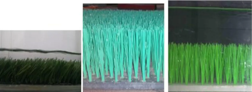
Fig. 1. Picture of the vegetation used for experiments S1 (left), S2 (center) and S3 (right).
is solved for a uniform and steady flow over vegetation. The analytical solution for velocity is computed considering the following turbulent shear stress τ:
𝜏 = ραududz (6) Where α (m) is a length scale. The velocity within the canopy is provided by the integration of the double averaged momentum balance. The boundary conditions for this integration in the vertical direction are no turbulence at the bed (Eq. (7)) and a shear stress at the canopy given by ρu*2. The
continuity at the top of canopy gives the values of the parameter d and z0.
𝑢0= √2𝑔𝑆𝑎𝐶
𝑑 (7) The correlation given by Klopstra et al. (1997) of α is:
𝛼
ℎ𝑝= 0.0793ℎ𝑝ln (
𝐻
ℎ𝑝) − 0.0009 (8) The influence of H could be linked to the penetration depth or a parameter of the mixing layer usually used in a two-layer model (Konings et al. 2012; Nepf, 2012; Nikora et al. 2013; Katul et al. 2011; Carollo et al. 2002).
This model will not be directly evaluated because the Eq. (8) was obtained with too few experiments. However, the following models reuse the same assumption and flow description.
2.4. Meijer, 1999/ Defina and Boixo, 2005 In the continuation of the Klopstra work, Meijer and Velzen (1999) carried out experiments to improve correlation on α for real vegetation. The calibration had revealed that the ratio H/hp is also necessary to well understand the results. They established a new turbulent closure (Eq. (9)):
𝛼
ℎ𝑝= 0.0144√
𝐻
ℎ𝑝 (9) 2.5. Cassan and Laurens, 2016
With the same concept, the length scale of the turbulent closure is calibrated with experiment series with rigid stems reported by Poggi et al. (2009) and experiments with cylindrical
macro-roughness. The vegetation density is expressed as a ratio of area in a horizontal plane, C = mD2. The
length is scaled considering the geometrical distance, s, between stem or hp the stem height. This
choice was made to integrate flow description in
Huthoff et al. (2007). To consider the influence of the upper layer, the length scale is related to the upper flow and it is coupled to the lower layer flow by the turbulent viscosity continuity. This assumption, regarding the turbulent properties at the top of canopy has provided good results for rigid vegetation and low submergence. Therefore, the Eq. (9) is substituted by the Eq. (l0).
𝑙 = min(0.15ℎ𝑝, 𝑠) (10)
The drag coefficient is also modified to take into account the ratio between hp and D and the flow
interaction with the bed. These corrections were necessary to ensure the continuity between the emergent and submerged vegetated flows. Finally, the vertical velocity distribution is given by the Eq. (11) for the lower layer.
𝑢(𝑧̃) = 𝑢0√𝛽(ℎ𝐻 𝑝− 1) 𝑠𝑖𝑛ℎ(𝛽𝑧)̃ cosh(𝛽)+ 1 (11) With ² =ℎ𝑝 𝛼 𝐶𝑑𝐶ℎ𝑝/𝐷 1−𝜋/4𝐶 , 𝑧̃ = 𝑧/ℎ𝑝 is the dimensionless vertical position. 2.6. Experiments
The first experiments concerned a flexible vegetated bottom at the INAT (National Institute of Agronomy of Tunisia) laboratory in a rectangular channel 5 m long, and 0.075 m wide and 0.15 m deep. The aim is to compare the experimental results with the analytical models for very dense canopy. On the bottom, initially smooth, we glued, in the longitudinal direction of the flow a vegetation cover that has 40 mm as height of fibers distributed in the center of the channel as indicated in Fig. 1. The number of stems is obtained by counting them of an area of 5 cm by 5 cm. The water depth is measured by analyzing side views from a camera (640*230 pixels with 1 pixel=0.625 mm).
The second series of experiments were conducted in a flume 5.75 m long and 0.29 m wide (Montpellier Supagro, France). The bed was covered with artificial flexible vegetation made with thin circular
H. Romdhane et al. / JAFM, Vol. 12, No. 2, pp. 351-359, 2019.
354
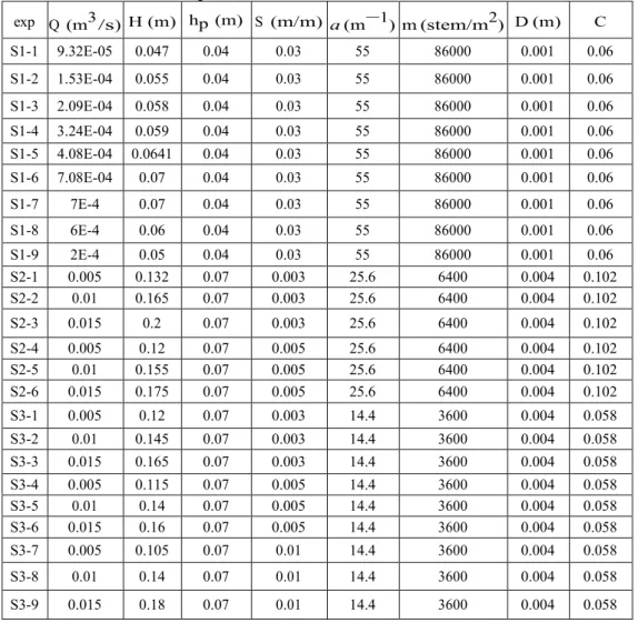
Table 1 Experimental results for 3 types of dense vegetation. For S2 and S3, D corresponds to the equivalent diameter due to several stems
exp Q (m3 /s) H (m) hp (m) S (m/m) a (m−1) m (stem/m2) D (m) C S1-1 9.32E-05 0.047 0.04 0.03 55 86000 0.001 0.06 S1-2 1.53E-04 0.055 0.04 0.03 55 86000 0.001 0.06 S1-3 2.09E-04 0.058 0.04 0.03 55 86000 0.001 0.06 S1-4 3.24E-04 0.059 0.04 0.03 55 86000 0.001 0.06 S1-5 4.08E-04 0.0641 0.04 0.03 55 86000 0.001 0.06 S1-6 7.08E-04 0.07 0.04 0.03 55 86000 0.001 0.06 S1-7 7E-4 0.07 0.04 0.03 55 86000 0.001 0.06 S1-8 6E-4 0.06 0.04 0.03 55 86000 0.001 0.06 S1-9 2E-4 0.05 0.04 0.03 55 86000 0.001 0.06 S2-1 0.005 0.132 0.07 0.003 25.6 6400 0.004 0.102 S2-2 0.01 0.165 0.07 0.003 25.6 6400 0.004 0.102 S2-3 0.015 0.2 0.07 0.003 25.6 6400 0.004 0.102 S2-4 0.005 0.12 0.07 0.005 25.6 6400 0.004 0.102 S2-5 0.01 0.155 0.07 0.005 25.6 6400 0.004 0.102 S2-6 0.015 0.175 0.07 0.005 25.6 6400 0.004 0.102 S3-1 0.005 0.12 0.07 0.003 14.4 3600 0.004 0.058 S3-2 0.01 0.145 0.07 0.003 14.4 3600 0.004 0.058 S3-3 0.015 0.165 0.07 0.003 14.4 3600 0.004 0.058 S3-4 0.005 0.115 0.07 0.005 14.4 3600 0.004 0.058 S3-5 0.01 0.14 0.07 0.005 14.4 3600 0.004 0.058 S3-6 0.015 0.16 0.07 0.005 14.4 3600 0.004 0.058 S3-7 0.005 0.105 0.07 0.01 14.4 3600 0.004 0.058 S3-8 0.01 0.14 0.07 0.01 14.4 3600 0.004 0.058 S3-9 0.015 0.18 0.07 0.01 14.4 3600 0.004 0.058
cylinders of 0.8 mm diameter. A dozen of cylinders were gathered and stuck on a PVC blade at the same position. Then the diameter of a stem is 4 mm. These basic vegetation cylinders were set in a staggered arrangement with 2 different distances between stems corresponding to 2 different densities. The cylinder height is equal to 7 cm (Fig. 1). The spatial density, which is equal to mD = C/D, remains almost constant in the vertical direction although near the canopy cylinders are no more contiguous.
The flume slope could be adjusted from 0 to 3 %. A weir at the upstream end allows fixing different water depths. The flow discharge was measured with an electromagnetic flowmeter with an uncertainty lower than 1%.
Velocity profiles above the vegetation is obtained by Acoustic Doppler velocimetry with an micro-ADV Nortek Vectrino+ with a sample sampling rate equal to 25 Hz. The vegetation is assumed to be dense enough to cause a velocity profile independent of the lateral position relatively to the arrangement. The velocity measurements were performed for experiments 2, 3, 5 and S3-6.
3. RESULTS AND DISCUSSION 3.1. Velocity Profiles
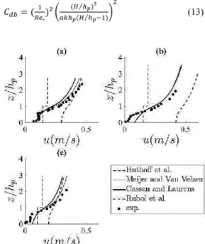
The velocity distribution calculation with the models from Defina and Bixio (2005),Cassan and Laurens (2016) and Rubol et al. (2018) had been validated for several experiments. But the comparison for a dense case is difficult because of the measurement within the canopy. In addition of the present velocity measurements (Fig. 2), the experiment from Le Bouteiller and Venditti (2015)
for dense vegetation which has never been compared to double averaged model, is particularly adapted because of their plant densities and simple canopy configuration. The Fig. 3 presents the velocity profiles for Cd =1 where Re∗ is 4200, 4600
and 3300. Similarly, the experiments with flexible vegetation and various densities could be used (Kubrak et al., 2008) to precise the role of velocity within the canopy.
The Huthoff’s model appears to be the less pertinent to compute accurate discharge, the calibration of the model was performed for sparser vegetation which could explain the discrepancies. However for the S3
experiments, the gap with experiments is reduced. Then a new calibration could be studied to keep the simplicity of the model but enlarging the range of applicability.
The Meijer and Cassan models are likely to better reproduce the velocity above the canopy and then the discharge. The flexible vegetation can be considered as rigid using the deflected heigth. The velocity computed with the Rubol model can differs greatly from experiments, in particular within the canopy. But the experiments chosen may be too sparse as regard of the validity range of the Darcy-Brinckman equation. This issue appears clearly by analysing the Kubrak’s experiments where a good agreement is observed for the denser canopy (Fig. 4) but the difference increases when the density decreases. For the two first curves (a=9 m−1), the model provides a consistent discharge whereas for other experiments (a=2.25 m−1) the velocity is largely over estimated. Moreover, it must be kept in mind that the Rubol model could be improved by a better estimation of the permeability.
Fig. 2. Comparison of velocity profile of experiments S3-5 (a), S3-6 (b), S3-2 (c) and S3-3
(d) and the 4 models. 3.2. Friction Coefficient
For all models, the hydraulic resistance is described with a drag coefficient which expresses the drag force as a function of either the bulk velocity (Cdb)
(Rubol et al. 2018) or the velocity in the canopy (Cd) (other models).
With the first method in a steady uniform flow, the momentum equation on the water volume in the canopy is given by the equilibrium between shear stress at the canopy, the drag force and the water weight if the shear stress on bed is neglected. For the water volume around one stem, this consideration can be written as follows:
1 2𝐶𝑑𝑏𝐷ℎ𝑝𝑈𝑏 2=𝑢∗2 𝑚+ 𝑔𝑠ℎ𝑝 𝑚 (12)
Considering 𝑢∗= √𝑔𝑆(𝐻 − ℎ𝑝), the second term
can be written u*²/m(1+1/(H/hp-1)). Rearranging
Eq. (12), one obtains : 𝐶𝑑𝑏= (𝑅𝑒1 ∗)² ( (𝐻 ℎ⁄ 𝑝)3 𝑎𝑘ℎ𝑝(𝐻 ℎ⁄ 𝑝−1)) 2 (13)
Fig. 3. Comparison of velocity profile of (Le Bouteiller and Venditti, 2015) experiments and
the 4 models. Re∗ =4200 (a), 4600 (b) and 3300 (c).
Fig. 4. Comparison of velocity profiles of (Kubrak et al., 2008) experiments and the 4 models. The figures correspond respectively to the experiments 1.1.3 (a), 1.2.1 (b), 2.2.1 (c), 3.1.1
(d), 3.2.1 (e), 4.1.1 (f), 4.2.1 (g).
Usually the experiments with flexible vegetation are performed for a limited range of ratio H/hp
(between 1 and 4) and density (ahp) between 1 and
10 m−1. On the other hand, the variations of 𝑅𝑒∗are
quite larger, therefore it was effectively observed that CdB decreases with the Reynolds number 𝑅𝑒∗
(Fig. 5) (Wilson, 2007) corresponding to the first term in parenthesis in the Eq. (13).
H. Romdhane et al. / JAFM, Vol. 12, No. 2, pp. 351-359, 2019.
356 Fig. 5. Drag coefficient based on the bulk velocity as a function of Re∗ (ahp =3 in Eq. (13)).
The experimental results from Rubol et al. (2018)
shows that CdB scale as 𝑅𝑒∗−𝛾 with γ=1.38.
However, these measurements are significant only if the term ( (𝐻 ℎ⁄ 𝑝)3
𝑎𝑘ℎ𝑝(𝐻 ℎ⁄ 𝑝−1))
2
is almost constant, otherwise the Eq. (13) could be finally another expression of the momentum balance with a constant friction coefficient. Formula using a Reynolds number based on the bulk velocity and molecular viscosity should be more relevant.
For the experiments from the present study, from Le Bouteiller and Venditti (2015) and those reported by Poggi et al. (2009), the general trend of CdB is
actually given by Re*2 for experiments with
artificial stripes whereas the γ=1.38 agrees with the experiments with real vegetation (Carollo et al. 2002; Ciraolo and Ferreri 2007). From Fig. 5, it can be stated that the experimental correlation from
Rubol et al. (2018) is enough accurate for real dense vegetation. It also could be the evidence that the friction in the canopy does not depend on the square velocity (γ ≠ 2). In other words, the viscous term or stem vibration on drag can be significant. However, it seems that the variation of CdB from
experiments could be also explained by a variation of H/hp. As it is not possible to discriminate
between the two explanations, this method is not studied further, and we focused on the velocity integration profile.
For experiments with artificial stems, the second method (with Cd) was developed to link the
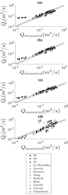
hydraulic resistance to fluid mechanical process in the canopy. As explained above, the main challenge is to well model the turbulence in the mixing layer at the top of the canopy because it is responsible for the velocity profile in the upper layer. For dense canopy, the larger part of the discharge flows in the upper layer, then it is crucial to well described the velocity profile. The comparison between computed discharges (Qc) with the 4 models is drawn on the Fig. 6. The Huthoff model shows a good agreement for a large number of experiments and it is less efficient than others even if it is simpler. The difference occurs mainly for the denser canopies:
present experiments and those of (Carollo et al. 2002; Ciraolo and Ferreri 2007). For experiments with real vegetation (Carollo et al. 2002; Ciraolo and Ferreri 2007), the model performance is generally worse than for the experiments with stripes. It could be easily explained by the fact that Cd is assumed to be equal to 1 whereas it
should integrate a Reynolds or a shape dependence due to leaves. For the Meijer model a discrepancy is noticed for the present’s experiments (S1). The model from Cassan and Laurens (2016) improves slightly the Meijer’s one by reducing the computed discharge thanks to a new formulation of the drag coefficient and turbulent length scale. Although the permeability
K is not calibrated, the most efficient model is the
Rubol’s model which provides a very good agreement for the majority of experiments. However for some series (Kubrak et al. 2008;
Yang and Choi 2009), the measured discharges differ from the computed ones.
To understand the reason of the discrepancies, the error between the computed and measured discharge is depicted on the Fig. 7 as a function of the Reynolds number based on the molecular viscosity Re=UH/ν. As expected, the Rubol’s model reproduces satisfactorily the discharge for the lower Reynolds number. The other models become pertinent only for Re>20000. The averaged accuracy could be estimated to 30 %. For the low Re, it could be stated that the model provides a better discharge prediction because it is the only one which can reproduce the increase of the drag coefficient for low Reynold flow. At high Re number the efficiency of this model decreases and those developed for fully turbulent flow and sparser canopy become more pertinent.
4 CONCLUSION
A description of the hydraulic resistance due to a flexible and dense vegetation is necessary to calculate the flows in the natural cases. The analytical models studied can give an estimation of the discharge. The role of the viscous term in the dense canopy has been emphasized since the model based on the Darcy-Brinckman equation provides performant result. Indeed, the most accurate model for friction prediction is the one of Rubol et al. (2018) which already integrates a low Reynolds number into the resolved physical law. This model depends on the canopy permeability and its formulation from Happel (1959) gives a relevant approximation similarly than study on rigid vegetation (Battiato et al. 2014). Further experimental studies are needed to improve calibration of this model, because measurements of permeability vegetation may be difficult in the field. For a higher Reynolds number flow, the analytical models (Meijer and Velzen, 1999; Cassan and Laurens, 2016) allows computing a vertical velocity distribution and they are relevant for replicating experimental results over a wide range of hydraulic conditions. Finally, it may be interesting to have later relevant models that will be applied for studies
with an intermediate Reynolds number.
Fig. 6. Comparison of the total discharge over vegetated bed for the model of Huthoff (a), the Meijer and Van Velzen (b), Cassan and Laurens
(c), and Rubol et al. (d) (Cd =1 for all experiments). Experiments from (Le Bouteiller and Venditti, 2015; Jarvela, 2005; Kouwen and Unny, 1969; Yang and Choi, 2009; Kubrak et al.,
2008; Huai et al., 2009; Carollo, Ferro, Termini, 2002; Ciraolo, Ferreri, 2007; Ghisalberti and Nepf, 2006). Dash lines represents a deviation of
30 %.
Fig. 7. Error between the 4 models and experiments from literature (Le Bouteiller and
Venditti, 2015; Jarvela, 2005; Kouwen and Unny, 1969; Yang and Choi, 2009; Kubrak et al.,
2008; Huai et al., 2009; Carollo, Ferro, Termini, 2002; Ciraolo, Ferreri, 2007; Ghisalberti and
Nepf, 2006) as a function of the Reynolds number.
REFERENCES
Battiato, I. and S. Rubol (2014). Single-parameter model of vegetated aquatic flows. Water
Resources Research 50, 63586369.
Carollo F. G., V. Ferro and D. Termini (2002). Flow velocity measurements in vegetated channels Journal of Hydraulic Engineering 128(7), 664.
Cassan, L., H. Roux and P. A. Garambois (2017). semi-analytical model for the hydraulic resistance due to macro-roughnesses of varying shapes and densities. Water 9(637), 2–18. Cassan, L. and P. Laurens (2016). Design of
emergent and submerged rock-ramp fish passes Knowl. Manag. Aquat. Ecosyst. (417), 45. Cheng, N. and H. Nguyen (2011). Hydraulic radius
H. Romdhane et al. / JAFM, Vol. 12, No. 2, pp. 351-359, 2019.
358
for evaluating resistance induced by simulated emergent vegetation in open-channel flows
Journal of Hydraulic Engineering 137(9), 995–
1004.
Ciraolo, G. and G. B. Ferreri (2007). Log velocity profile and bottom displacment for a flow over a very flexible submerged canopy 32nd Congres: Harmonizing the Demands of Art and Nature in International Association of Hydraulic Engineering and Research.
Defina, A. and A. Bixio (2005). Mean flow turbulence in vegetated open channel flow.
water resources research 41, 1–12.
Douinot, A., H. Roux and D. Dartus (2017). Modelling errors calculation adapted to rainfall runoff model user expectations and discharge data uncertainties. Environmental Modelling
and Software 90, 157-166.
Ghisalberti, M. and H. M. Nepf (2006). The structure of the shear layer in flows over rigid and flexible canopies. Environmental Fluid
Mechanics 6, 277–301.
Happel, J. (1959). Viscous flow relative to arrays of cylinders. AIChE Journal 5, 174–177.
Huai, W. X., Z. B. Chen, J. Han, L. X. Zhang and Y. H. Zeng (2009). Mathematical model for the flow with submerged and emerged rigid vegetation. Journal of Hydrodynamics, Serie B 21(5), 722 – 729.
Huthoff, F., D. C. M. Augustijn and S. J. M. H. Hulscher (2007). Analytical solution of the depth-averaged flow velocity in case of submerged rigid cylindrical vegetation. Water
Resources Research 43(6), W06413.
Jarvela, J. (2005). Effect of submerged flexible vegetation on flow structure and resistance.
Journal of Hydrology 307(1-4), 233 – 241.
Katul, G. G., D. Poggi and L. Ridolfi (2011). A flow resistance model for assessing the impact of vegetation on flood routing mechanics.
Water Resources Research 47(8), 1–15.
King, A. T., R. O. Tinoco and E. A. Cowen (2012). A k- turbulence model based on the scales of vertical shear and stem wakes valid for emergent and submerged vegetated flows.
Journal of Fluid Mechanics 701, 1–39.
Klopstra, D., H. Barneveld, J. Van Noortwijk and E. Van Velzen (1997). Analytical model for hydraulic resistance of submerged vegetation.
Proceedings of the 27th International Association of Hydraulic Engineering and Research Congress, 775–780.
Konings, A. G., G. G. Katul and S. E. Thompson (2012). A phenomenological model for the flow resistance over submerged vegetation. Water
Resources Research 48(2).
Kouwen, N. and T. E. Unny (1969). Flow retardance in vegetated channels. Journal of the
Irrigation and Drainage Division 95(2), 329–
344.
Kubrak, E., J. Kubrak and P. M. Rowinski (2008). Vertical velocity distributions through and
above submerged, flexible vegetation.
Hydrological Sciences Journal 53(4), 905–920.
Kucukali, S. and R. Hassinger (2018). Flow and turbulence structure in a baffle-brush fish pass. Proceedings of the Institution of Civil Engineers - Water Management, 171(1): 6–17.
Le Bouteiller and C. J. G. Venditti (2015). Sediment transport and shear stress partitioning in a vegetated flow. Water Resources Research 51.
Liu, C. and Y. M. Shen (2008). Flow Structure and Sediment Transport with Impacts of Aquatic Vegetation. Journal of Hydrodynamics 20(4), 461468.
Marjoribanks, T., R. J. Hardy, S. Lane and D. R. Parsons (2017). Does the canopy mixing layer model apply to highly flexible aquatic vegetation Insights from numerical modelling.
Environmental Fluid Mechanics 17(2), 277–
301.
Meijer, D. G. and E. H. Van Velzen (1999). Prototype scale flume experiments on hydraulic roughness of submerged vegetation. 28th
International International Association for Hydro-Environment Engineering and Research.
Morri, M., A. Soualmia and P. Belleudy (2015). Mean Velocity Modeling of Open-Channel Flow with Submerged Rigid Vegetation. .
World Academy of Science, Engineering and Technology, International Journal of Mechanical, Aerospace, Industrial, Mechatronic and Manufacturing Engineering 9
(2), 302-307.
Murphy, E. G. and H. Nepf (2007). Model and laboratory study of dispersion in flows with submerged vegetation. Water Resources
Research 43(5), 1–12.
Nepf, H. M. (2012). Hydrodynamics of vegetated channels. Journal of Hydraulic Research 50(3), 262–279.
Nikora, N., V. Nikora and T. O Donoghue (2013). Velocity profiles in vegetated open-channel flows: Combined effects of multiple mechanisms. Journal of Hydraulic Engineering 139(10), 1021–1032.
Nikora, V., D. Goring, I. McEwan and G. Griffiths (2001). Spatially averaged open-channel flow over rough bed. Journal of Hydraulic
Engineering 127(2), 123–133.
Poggi, D., A. Porporato and L. Ridolfi (2004). The effect of vegetation density on canopy sub-layer turbulence. Boundary-Layer Meteorology 111, 565–587.
Poggi, D., C. Krug and G. G. Katul (2009). Hydraulic resistance of submerged rigid vegetation derived from first-order closure
models. Water Resources Research 45(10). Rubol, S., B. Ling and I. Battiato (2018). Universal
scaling-law for flow resistance over canopies with complex morphology, Scientific Reports, 8, 4430
Wilson, C. A. M. E. (2007). Flow resistance models for flexible submerged vegetation. Journal of
Hydrology 342(3-4), 213-222.
Wu, W. and Z. He (2009). Effects of vegetation on flow conveyance and sediment transport capacity. International Journal of Research 23(3), 47-259.
Yang, W. and S. U. Choi (2009). Impact of stem flexibility on mean flow and turbulence structure in depth- limited open channel flows with submerged vegetation. Journal of