Aerodynamic simulation strategies assessment for a Fenestron® in hover flight

O

pen

A

rchive

T

OULOUSE

A

rchive

O

uverte (

OATAO

)

OATAO is an open access repository that collects the work of Toulouse researchers and

makes it freely available over the web where possible.

This is an author-deposited version published in:

http://oatao.univ-toulouse.fr/

Eprints ID: 17416

To cite this version: Marino, Morgane and Gourdain, Nicolas and Legras, Guillaume and

Alfano, Davide Aerodynamic simulation strategies assessment for a Fenestron® in hover

flight. (2015) In: 6th European conference for aeronautics and space sciences (EUCASS),

Aerodynamic simulation strategies assessment for a Fenestron

®

in hover flight

Marino Morgane*, Gourdain Nicolas †, Legras Guillaume ‡ and Alfano David ‡ *PhD Candidate

Airbus Helicopters SAS, 13725 Marignane, France and CERFACS, 31057 Toulouse, France

†_{Professor, Department of aerodynamics, energetics and propulsion}

ISAE Sup’Aero, 31400 Toulouse, France

‡_{Engineer, Aerodynamics department}

Airbus Helicopters SAS, 13725 Marignane, France

Abstract

The Fenestron® _{has a crucial anti-torque function and its sizing is a key point of the Helicopter design,}

especially regarding thrust and power predictions. This paper reports the investigations done on a full scale Dauphin Fenestron®_{. The objectives are first to evaluate the influence of some numerical parameters on the}

performance of the Fenestron®. Then the flow is analyzed for a high incidence pitche, for which the rotor blade can experience massive boundary layer separations. Simulations are carried out on a single blade passage model. Several parameters are benched, such as grid quality, numerical schemes and turbulence modeling. A comparison with test bench measurements is carried out to evaluate the capability of the numerical simulations to predict both global performance (thrust and power) and local flows (static pressure at the shroud and radial profiles inside the vein). The analysis demonstrates the capability of numerical simulations to accurately estimate the global performance of the Fenestron®_{, including at high pitch angles.}

However, some discrepancies remain on the local flow, especially in the vicinity of the rotor shroud. A more detailed analysis of the local flow is performed at a blade pitch angle of 35°, with a particular interest for the blade tip region.

Abbreviations

AUSMP Advection Upstream Splitting Method CFD Computational Fluid Dynamics

elsA ensemble logiciel de simulation en Aérodynamique JST Jameson Schmidt Turkel

L-S Launder Sharma

MUSCL Monotone Upwind Scheme for Scalar Conservative Laws RANS Reynolds-Averaged Navier-Stokes

S-A Spalart-Allmaras SST Shear Stress Transport

Nomenclature

FT Fenestron® _{Thrust [DaN]}

FP Fenestron® Power [kW] h Radial position in the

vein

[m] H Height of the vein [m] h/H Normalized radial position [ - ] k Turbulence kinetic energy [m2_.s-2] Vz Axial velocity [m.s-1] VTIP Blade tip velocity, RΩ [m.s-1]

y+ Non-dimensional wall distance [ - ]

ρ Density [kg.m-3]

ε Rate of turbulence kinetic energy dissipation

[m2.s-3] ω Frequency of turbulence kinetic energy [s-1] Ω Rotation speed

CFT Fenestron® _{Thrust coefficient,} !"

Q Mass flow [kg.s-1] p Static pressure [Pa] p∞ Ambient pressure [Pa] R Shroud radius [m]

CFP Fenestron® _{Power coefficient} !" !∗!∗!!_∗! !"#! [ - ] C_! Pressure coefficient, ( !!!! ! !∗!∗!!"#! ) [ - ]

1. Introduction

The Fenestron® _{was developed by the engineering department of Sud-Aviation (Airbus Helicopters) in}

1970’s [5] [6] as an alternative solution to the conventional tail rotor. The principal function of the Fenestron® _{is to}

generate a thrust to counterbalance the torque of the main rotor. Improvements, in terms of safety and noise, for light-to-medium helicopters, have made it a trademark for Airbus Helicopters. The system is composed of a shrouded rotor and topped with a large vertical fin [3], as described on Figure 1. The shroud includes a collector with rounded lips, a cylindrical zone at the blade passage and a conical diffuser. The gearbox (hub) is supported by three arms or a stator row and fairs systems which provide power to the rotor and control the blade pitch angle. The pitch rotor monitors the rotor thrust of the Fenestron®. In hover flight, the rotor (fan) leads the flow from the collector to the diffuser which creates the shroud effort. The thrust of the Fenestron® _{is thus composed by the shroud}

and the rotor thrust.

Figure 1: overview of the Fenestron® _principle

The sizing of the Fenestron® is still a challenge, due to the complexity of the flow. The internal flow of the Fenestron® is three-dimensional, turbulent and unsteady due to the interactions between fixed (shroud-stator) and rotating parts (rotor). Like in most turbomachines, secondary flows also exist in the Fenestron®_{, such as the tip}

leakage flow induced by the clearance between the rotor and the shroud. As a consequence, the analysis of the flow in realistic industrial configurations remains very difficult, even in a wind tunnel environment. Supported by experimental campaigns [3]-[8], a better understanding of the flow physics in these systems can be expected thanks to recent progresses in Computational Fluid Dynamics (CFD).

Several numerical approaches have been proposed in the literature to represent the flow in Fenestron® configurations. For example the use of a 2D-axisymmetric model has been carried out on the Dauphin helicopter in hover flight, showing good agreement with measurements [3]. However, this approach can be used only for axial flight conditions and 3D effects, such as blade tip vortices, are not represented. Another way to model the flow in the Fenestron® consists in solving Navier-Stokes equations on a 2D-axisymmetric shroud and by modeling the fan as a fully coupled, time averaged momentum source term in the momentum equation [9]. While numerical predictions were in good agreement with measurements in the collector area, the pressure distribution was not accurately estimated in the blade region [9]. Other works reported in the literature suggest to use an approach based on a 3D geometry of the shroud [11]-[12]-[13]. The rotor is modeled by an actuator disk that uses the momentum and blade element theory to estimate the rotor thrust corresponding to a single pitch. The major benefit of the model is the computational cost reduction due to the rotor simplification. This approach allows computing the Fenestron®

performance in the whole flight domain. However, this method does not represent 3D effects in the vicinity of the blade, such as tip clearance and blade swirl. It usually results in an unrepresentative local flow into the vein [13]. To improve the quality of the numerical predictions for 3D flows, the solution is thus to consider the full 3D domain with rotating (rotor) and fixed (shroud-hub-stator-fin) parts [15]. The advantages of this method are the accuracy of

consuming in terms of both mesh generation and simulation time. To balance the simulation cost, it is possible to reduce the whole domain to a single blade passage with spatial periodic conditions [2]. This approach has been validated in hover flight on the EC135 geometry [15]. Despite the increase of the available computing power, only a few studies deal with the validation of the numerical method for 3D flows, as reported in [15]. The scope of this paper is thus to evaluate the influence of numerical parameters (mesh, scheme and turbulence) on the global performance and local flows of the Fenestron® _{in hover flight.}

To validate the method, numerical predictions are compared to bench test measurements on a full scale Dauphin Fenestron® _{[3]. The CFD approach is based on the single blade passage proposed by Mouterde in [9]. Since}

this work focuses on the local flow and interactions between the rotor and the shroud, the stator is not modeled in order to simplify the geometry. The numerical simulation of the flow relies on a representation of the 3D flow with a Reynolds-Averaged Navier-Stokes (RANS) approach (all turbulent scales are modeled). The first part of the paper details the experimental test case and computational setup. Then the second part of the study proposes an evaluation of the meshing strategies. The Chimera technique is compared to a fully coincident meshing approach. For the chimera technique an evaluation of the meshing refinement is conducted. The third part of the paper proposes to evaluate the influence of numerical schemes and turbulence modeling on the prediction of the Fenestron® performance.

2. Study case

2.1 Experimental case

The test case investigated in this paper is the Dauphin Fenestron® _{investigated by Morelli and Vuillet [3].}

Experiments were carried out on a scale one test bench in hover flight. Measurements on the ducted rotor have been done to compare different rotor and shroud configurations. Among the different configurations described by Morelli and Vuillet [3], the reference case is chosen. It is based on a rotor with 11 equally spaced blades and a hub supported by three arms. A balance (with an accuracy of 1%) and a torque system (with an accuracy of 0.5%) are used to measure thrust and power. As illustrated in Figure 2, the local flow is evaluated by measuring the static pressure with 32 steady sensors located along the duct vein. The flow is also characterized upstream and downstream the rotor at several radial locations with a 5-hole probe.

Figure 2: Locations of static pressure measurements at the shroud (from Morelli and Vuillet [3])

2.2 Computational setup

The numerical simulations are performed with the code elsA, developed at ONERA [1]. This solver is a multidisciplinary code object-oriented, specialized in both internal and external flows. This code solves both Euler and Navier Stokes equations. It is based on a cell-centered finite volume formulation on multi-block structured meshes. A wide panel of turbulence models and numerical schemes is available. The study reported in this paper relies on a steady-state RANS approach. Boundary layers are assumed to be fully turbulent due to the large Reynolds number, based on the rotor chord (Re > 106_{). As reported in the literature [26], there are four main sources}

of errors when comparing numerical predictions with experimental data:

- Accuracy of the simulated geometry (and difficulty to represent small details such as technological effects), - Boundary conditions (e.g. isothermal or adiabatic walls, far-field approximation),

- Adequacy between the numerical scheme (spectral properties of the scheme) and the mesh grid quality, - Turbulence modeling (RANS, LES, etc.).

This work specifically handles the two last sources of errors (discretization and turbulence modeling errors). To do this, different meshing approaches, numerical schemes and RANS-based turbulence models are benched and their influence on the global performance and local flows predictions are evaluated. For all computations, a 3D single blade passage is chosen. Periodic conditions are applied on the lateral faces of the domain. Far-field boundary conditions are used for the external boundaries of the domain. The size of the domain is 10.R in each direction (with

R the radius of the Fenestron®_{) around the shroud geometry. Previous simulations have been run with a 20.R}3 _{box to}

check that the size of the domain has no influence on local flow and global performance predictions. Shroud, hub and blade walls are represented with non-slip boundary conditions. The rotor rotates around the Z-axis and the blade pitch axis is defined as the Y-axis as shown in Figure 3.

3. Meshing strategy for Fenestron

issues

For structured multi-block meshes, the main difficulty lies on the grid generation process around complex geometries. Concerning the Fenestron®_{, the blade pitch variation [-10°; +40°] and the rotor tip clearance represent a}

considerable challenge for the grid topology and the mesh quality.

First, in order to choose the correct meshing strategy, the coincident approach is compared to the chimera method. The coincident approach is the reference method to simulate with accuracy the geometry. Nevertheless, with a variation of 50° of pitch angle, a given grid topology is not adapted for all blade pitches [15] (so the meshing should be adapted to each blade pitch, which is not affordable to describe the whole performance curve). The second meshing strategy is the Chimera method [13] [28]. The advantage of the Chimera approach is to segregate the mesh generation of fixed and rotating parts. Nevertheless, the overset method induces conservation losses through the interpolations between meshes. Moreover fixed and rotating cannot be fully encased without an overlapped grid or a gap between them. Then, the second part of the work proposes an evaluation of the grid refinement for the chimera method. The aim is to compare four grid refinements to evaluate the influence on the performance of the Fenestron® and on the rotor wake dissipation. All calculations presented in this section are carried out with the two-equation turbulence model k-ω of Kok [20] and a 2nd _{order centered numerical scheme [23]. The first study is carried out on}

the M1 grid (see Table 1) with 6 million grid points.

3.1 Description of the coincident approach

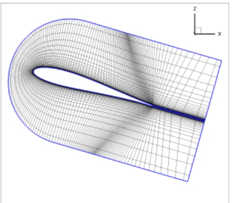
Two strategies can be used for the meshing of the Fenestron® with a coincident approach. On the one hand, D’Alascio et al. [15] generated the grid topology for high pitches and encounter difficulties for low blade pitches. On the other hand, the work reported in this paper proposes to mesh in the first instance the low pitches and to adapt the grid topology for high pitch cases. An O-grid topology is used for the shroud, hub and blade geometries. A H-topology is adopted for the blade tip area. The reference mesh is made of 156 blocks. The size of the first cell is imposed to achieve a normalized wall distance around unity (y+_{~1), which is mandatory to fully resolve boundary} layers. The blade grid at 50% of the span is presented on Figure 5, for a pitch of 25°.

3.2 Description of the Chimera approach

For the Fenestron® _{application, the Chimera method consists in separately generating blade and shroud-hub}

meshes which permits to easily set up the pitch around the blade pitch axis, as shown on Figure 3. The assembly of the two meshes is realized by the application of overlapping boundary conditions and masking conditions for areas corresponding to a solid. For both boundary conditions, the transfer of conservative and turbulent variables is done through 3D non-conservative interpolations. The Alternative Digital Trees (ADT) method [27] is used to solve the interpolation search cell procedure for fixed and rotating meshes. A second order interpolation is chosen to improve the accuracy of the interpolation with a particular care for grid consistence between the two meshes. An evaluation of the conservative losses inherent to the Chimera technique is proposed in Section 4.3. An encased problem is induced by the Chimera approach, which results in a non-physical root gap of a size similar to the shroud gap.

Figure 3 : Chimera grid assembly

The grid topology for the rotor blade is based on a C-H topology around the blade profile, as presented in Figure 4. Blade extremities (tip and root) are discretized by a H fluid volume topology. The first cell is set in order to obtain

y+_{=1 at wall. The whole blade mesh contains 22 blocks, representing 1.5x10}6 _{cells. The background mesh includes}

the shroud and the hub geometries. The grid generation is first done in 2D and is then extruded in a periodic 3D mesh. An O-block is chosen for the meshing of shroud and hub walls. The size of the first cell is also set to y+=1. The whole

background mesh is composed of 21 blocks and 4.5x106 _cells.

Figure 4: 2D view of the rotor grid with the Chimera approach at

h/H=0.85

Figure 5: 2D view of the rotor grid for the coincident approach at h/H=0.85

3.3 Comparison of the two strategies

This part is dedicated to the comparison between the coincident approach and the Chimera technique. It is first proposed to evaluate the conservative losses of the Chimera method, as it is performed for turbomachinery [29]. To quantify the losses induced by the overset method, the mass flow difference ΔQ is estimated from plane 1

(upstream the rotor) to plane 3 (downstream the rotor), as:

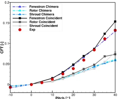
with Q the mass flow. The mass flow difference is close to 1.0% for a grid of 6x106 _{cells (grid M1). With the finest}

grid (grid M3, 23x106 _{cells) the mass flow loss reduces to 0.1%. Figure 6 compares numerical predictions with the}

two strategies to measurements. The global thrust as well as the shroud and the rotor thrusts are presented. According to the Froude theory [7], for both approaches, the total thrust of the system is the result of half rotor and shroud thrust (as also reported in wind tunnel campaigns [8]). Until a blade rotor pitch of +30°, the numerical predictions are not modified by the grid strategy. Then, from +30° to +40°, the coincident approach overestimates the Fenestron® _{thrust compared to measurements. This is related to an overestimation of the rotor thrust}

contribution. For analyzing the influence of the grid strategy on the local flow, normalized static pressure on the shroud for blade pitch +35° is presented on Figure 7. In the collector area, the static pressure distributions are equivalent for both strategies. It is coherent with the shroud polar curves observed in Figure 6. With the coincident

Q =

Q

Q

Q

approach, the static pressure distribution is affected by the mesh discretization, in the vicinity of the blade (Figure 7b). As a consequence, periodic blade wakes are quicker dissipated compared to the Chimera approach, due to the low-quality grid in the region of the shroud.

For the Chimera approach, Figure 8 points out the dissipation of the rotor wake at the trailing edge due to the interpolation inherent to the method. With the coincident approach, the wake is not dissipated but the resolution of the flow around the leading edge is influenced by the mesh quality.

To conclude, the Chimera approach is better adapted than the coincident approach, to describe the flow in a large range of blade pitches. To overcome this limitation, the coincident grid should be redesigned for each blade pitch, which is a costly task if automatic adaptive grid methods are not available. At this step, the use of the Chimera approach is thus preferable.

Figure 6: Comparison of the thrust coefficient between Chimera technique, the coincident approach and measurements

a) Chimera strategy b) Coincident strategy

Figure 7: Flow field for Chimera and coincident approaches for pitch 35°

Figure 8 : Axial velocity iso-contours at h/H=0.85 on coincident and Chimera approach

3.4 Analysis of grid refinement

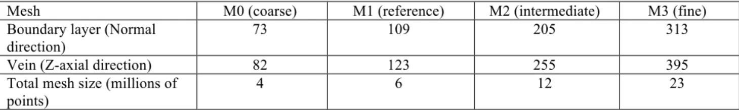
The effect of grid refinement is carried out for 4 different grids, from 4x106 cells (grid M0) to 23x106 cells (grid M3), as shown in Table 1. All computations in this section are performed with the two-equation turbulence model of Kok [20] with the SST correction and a 2nd order centered scheme [23].

Mesh M0 (coarse) M1 (reference) M2 (intermediate) M3 (fine) Boundary layer (Normal

direction)

73 109 205 313

Vein (Z-axial direction) 82 123 255 395 Total mesh size (millions of

points)

4 6 12 23

Table 1: Mesh grid refinement Global performance predictions

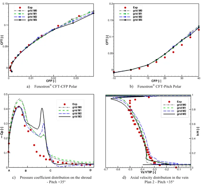
A comparison of the numerical prediction with the bench test is carried out on Figure 9 a) and b). The higher the pitch, the more the performance prediction is sensitive to grid refinement. A coarse mesh overestimates the thrust at blade pitches higher than +35o_{. A better grid refinement reduces the difference with measurements.} Local performance predictions

The effect of the refinement is analyzed for high blade pitch (+35°). Figure 9 c) presents the pressure coefficient distribution through the vein (from the collector lip to the diffuser lip). The points A to D correspond to the shroud, as presented in Figure 2. From point A to B, the upper collector zone evolves in a low-pressure area, where the suction peak is reached at the maximal curvature radius. This region of the shroud generates most of the thrust. Then, in the blade region, from point B to C, the decrease of the pressure is related to the presence of the blade tip vortices. This phenomenon will be better described in part 5. Through the diffuser, from point C to point D, the pressure returns to the ambient static pressure value.

For all mesh refinements, numerical results and tests follow the same trend. The pressure on the collector is more sensitive to grid refinement than the rest of the flow. Only refinements above grid M1 are in good agreements with measurements. The numerical simulations with grids M2 and M3 predict a stagnation zone at the end of the collector and before the blade passage. On the diffuser area, the solution is sensitive to the junction of the blade with the diffuser.

The grid refinement has also an influence on the pressure peak.

Figure 9 d) shows the radial profile of the axial velocity, extracted from plane 2, as a function of the radial position in the duct. Blade velocity distributions are obtained using an azimuthal mass flow averaging. Three zones are underlined. The first zone, from h/H=0 to h/H=0.05, corresponds to the blade root region which is influenced by the non-physical root leakage flow. The second one is the “linear zone” of the rotor, from h/H=0.05 to h/H=0.9. The third area highlights the effect of blade tip vortices, for h/H>0.9. In the linear zone, numerical predictions follow the same trend as the measurements. The axial velocity is overestimated at both the shroud and the root. In the blade tip region, axial velocity is over predicted by 20% for the grid M0 to 30 % for the grid M3. This observation is correlated with the suction peak that is discussed in part 5.

Effect on the rotor wake

Figure 10presents the axial velocity at h/H=0.85 for the M1 and M3 grids at pitch +35° (the solution of the blade grid is overlapped on the background grid), in order to show the wake dissipation. As expected, the wake dissipation is reduced with the finest grid (M3). This observation is in agreement with conservatives losses described in section 4.3. Therefore to preserve the wake of the rotor blade, the radial refinement of the grid should by three times more important than with a coincident approach.

a) Fenestron® CFT-CFP Polar b) Fenestron® CFT-Pitch Polar

c) Pressure coefficient distribution on the shroud - Pitch +35°

d) Axial velocity distribution in the vein Plan 2 - Pitch +35°

Figure 10: Axial velocity iso-contours with h/H=0.85

4.

Numerical parameters

4.1 Influence of the numerical scheme

To complete the grid refinement study, the influence of the numerical scheme is estimated. Three classical numerical schemes are tested. The second order centered scheme of Jameson Schmidt Turkel (JST) [23] is compared with the 2nd _{order Advection Upstream Splitting Method (AUSMP+ (P)) [24] and a 3}rd _{order scheme of}

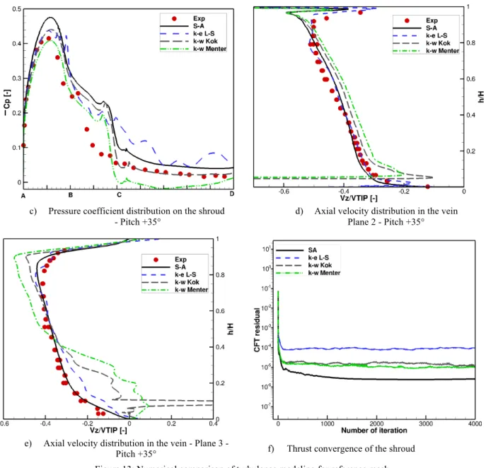
Roe [25]. To stabilize the JST scheme, an artificial viscosity term is added with a scalar artificial viscosity. The linear fourth order dissipation term k4 is set to 0.016. All simulations presented in this section are conducted on grid M1 with the two-equation turbulence model of Kok [20]. Figure 11 e) shows the convergence of the numerical solution for the three schemes. The residual decrease by three orders of magnitude, which is sufficient to consider that the convergence is achieved.

Global performance predictions

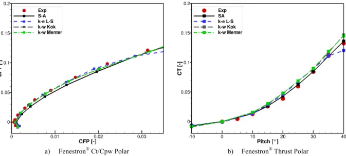
The numerical power prediction is compared to experimental data on Figure 11 a). For a high level of thrust, the increase of the scheme order improves the power estimation. However, on the thrust polar, Figure 11 b), the third order scheme of Roe overestimates the thrust compared to experimental data. For high pitch level, a balance is established between the accuracy of the power estimation, which needs a low dissipation from the numerical schemes, and the smoothing of the flow oscillations to reach the correct rate of thrust.

Local performance predictions

Figure 11 c) presents the pressure coefficient as a function of the vein distance for a blade rotor pitch of +35°, at the shroud. On the collector area, the pressure distribution is very sensitive to the numerical scheme. The JST scheme is in good agreement with the experimental bench data while the 3rd _{order scheme overestimates the}

static pressure coefficient at this location. Through the blade zone (from B to C) and in the vicinity of the diffusor, the solution is not sensitive to the numerical scheme. Figure 11 d) presents the axial velocity distribution on plane 2 for a blade rotor pitch of +35°, in the vein. The solution is not sensitive to the numerical schemes in the linear zone and in the vicinity of the blade tip. Indeed, the over-prediction of the velocity deficit in the tip region should not be attributed to the grid/scheme combination. Actually, most discrepancies are observed in the blade root region, as shown in Figure 11 e) at plane 3.

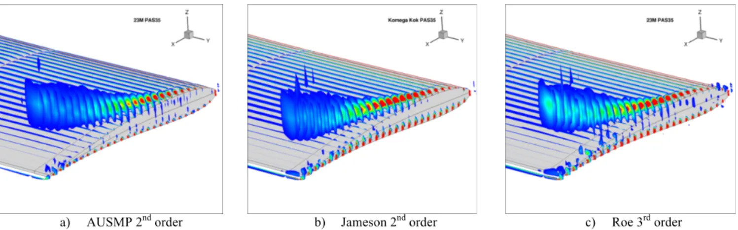
A qualitative study of the blade tip region has been conducted for blade rotor pitch +35°. The Q-criterion [30] is taken positive to point out the blade tip vortices, Figure 12. The convection of the tip vortex is influenced by the numerical scheme (the 3rd _{order scheme transports the tip vortex further downstream than 2}nd _{order schemes).}

The interaction between the blade vortex flow and the shroud is affected by the numerical scheme. The 3rd order

scheme predicts the development of small flow patterns that are not observed with 2nd _{order schemes. This}

mechanism is related to the creation of a “mirror vortex” at the shroud, as described by Cerra and Smith [31]. As a consequence, the wall induces the generation of a secondary vortex, rotating in the opposite direction. The mechanism is well shown in Figure 12, especially with the 3rd order scheme.

Actually, the sensitivity of the solution to the numerical scheme, especially the predictions of the power, increases with the blade pitch angle.

a) Fenestron® _{CFT-CFP Polar b) Fenestron}® _{CFT-Pitch Polar}

c) Pressure coefficient distribution on the shroud - Pitch

e) Axial velocity distribution in the vein - Plan 3 - Pitch

+35° f) Thrust convergence of the shroud

Figure 11: Numerical comparison of convective scheme for reference mesh

a) AUSMP 2nd _{order b) Jameson 2}nd _{order c) Roe 3}rd _order Figure 12: Comparison of Q positive function on the blade tip for different numerical schemes

4.2 Influence of turbulence modeling

The turbulence modeling is a key issue in RANS-based simulations. Different first order turbulence models are compared in this section: the one transport equation model of Spalart-Allmaras S-A [16] is compared with the two transport equations model of k-ε (Launder Sharma L-S) [18] and k-ω (Kok [20] and Menter [21]) with Shear Stress Transport (SST) correction. The SST correction proposed in [22] avoids the delay in the prediction of adverse pressure gradient effects. This correction should thus be helpful for the flow prediction at high pitch angles, for which the adverse pressure gradient is more important. All simulations presented in this section are performed on grid M1 with the 2nd _{order centered JST scheme. Figure 13 f) shows the convergence of the numerical solution with}

the four turbulence models. The residual drops by 3 or 4 orders of magnitude.

Global performance predictions

Figure 13 a) presents the power estimation depending on the turbulence modeling. In comparison with the experimental data, the thrust-power polars predicted by the Menter and Kok models overestimate at a high level of thrust. The S-A model reveals to be extremely dissipative. For the L-S model, a stall region appears. The thrust polar, shown on Figure 13 b), highlights two zones in comparison with experimental measurements. Two zones are observed: a first zone which is linear corresponds to low pitch angles, from [-10°; +35°] and a second zone which correspond to high pitch angles from [+35°; +40°]. In the linear zone, the two transport equation models (L-S, Kok, Menter) overestimate the thrust predictions compared to the S-A model. Differences increase at high blade rotor pitch. The L-S model predicts a region of stalled flow earlier compared to other models.

Local performance predictions

An analysis of the local flow is carried out on the blade rotor pitch angle of +35°. Pressure coefficient distributions at the shroud are presented on Figure 13 c). From point A to point B, at the inlet lip, turbulence models have an important influence on the pressure peak predictions, as shown in Table 2. The best agreement with measurements is observed with the k-ω model of Menter (error is 2% with respect to measurements).

Error in % Spalart-Allmaras k-ω Menter k-ω Kok k-ε Launder Sharma

-Cp 14 2 6 6

Table 2: Comparison of turbulence models with measurements for the prediction of the pressure peak coefficient, for a blade rotor pitch angle of +35°

A secondary increase of the pressure coefficient is observed with the L-S model, close to point B, which does not appear in the experimental measurements and with other turbulence models. However, all turbulence models show an increase of the pressure coefficient between point B and point C, related to the breakdown of the tip clearance vortex.

Figure 13 d) shows the radial profiles of normalized axial velocity at plane 2. The magnitude of the axial velocity is overestimated by most of turbulence models (except the L-S. k-ε model) compared to measurements, in the tip region (by about 20% with S-A. and k-ω models). This observation underlines the difficulty for first order turbulence models to accurately describe turbulence in the vicinity of the tip clearance. In the linear zone, h/H=0.05 to h/H=0.9, all turbulence models predict the same trend. At the blade root, k-ε and k-ω models are more influenced by the root leakage flow than other turbulence models. The S-A predicts a higher level of turbulent kinetic energy than other turbulence models, resulting in an increase of the turbulent viscosity. This behavior limits the non-physical root tip flow, which helps to match the measurements (however not for the good reasons).

Figure 13 e) shows the radial profiles of axial velocity distribution at plane 3. The differences between turbulence models predictions are more important at this section than at plane 2. The main reason is the influence of the size of the stalled flow that is predicted at plane 2, which impose a redistribution of the axial velocity inside the vein: if the mass flow is reduced at the shroud, it will increase the mass flow at the shroud. As for the prediction of the flow in the tip region at plane 2, it shows the difficulty to accurately predict the flow in such a configuration when separation occurs at high blade pitches.

This section shows that the global performance of the Fenestron® _{is sensitive to both numerical}

scheme and turbulence modeling. The power prediction is more influenced by the numerical schema while the thrust is more influenced by the turbulence modeling. For local performance, the turbulence modeling is of paramount importance in the vicinity of the blade tip clearance.

c) Pressure coefficient distribution on the shroud

- Pitch +35° d) Axial velocity distribution in the vein Plane 2 - Pitch +35°

e) Axial velocity distribution in the vein - Plane 3 -

Pitch +35° f) Thrust convergence of the shroud Figure 13: Numerical comparison of turbulence modeling for reference mesh

5. Comments on the blade region

In this section, the k-ω model of Kok and the 2nd centered order scheme of Jameson are used. The finest

grid M3 is chosen (23x106 _{cells) to conduct the local flow analysis in the vicinity of the blade. Most}

discrepancies between numerical predictions and measurements appear in the blade passage (from point B to point C). In this region two flow mechanisms interact together. First, the blade tip vortex is generated by the tip clearance, close to the shroud. Then the boundary layer of the shroud interacts with this vortex, leading to a secondary flow. This shear flow affects the tip region performance by promoting a three-dimensional separation [32]. Figure 15

presents a 3D view of the pressure coefficient, showing the effect of the blade tip vortex. The boundary layer of the shroud is sucked by the blade tip vortex therefore a suction peak appears in the coefficient of pressure (Figure 16). Such a suction peak has already been reported in the literature [9]. Such 3D flows are known to be challenging both for experimental sensors and numerical simulations, so it can explain, at least partially, the discrepancies between numerical simulations and measurements. However, since this part of the shroud is parallel to the streamwise flow, it does not affect the shroud thrust.

In order to highlight the difficulty to simulate the flow in the blade region, two pitches around the blade pitch angle of +35° are studied. “eps” is a small variation of the blade pitch around pitch +35° (about a degree). Figure 16 presents the distribution of the pressure coefficient for the three different pitches. The pressure coefficient distribution is well captured at the three pitch angles compared to measurements. Thereafter, the behavior of the suction peak in the blade region depends on the blade pitch angle. The higher the pitch angle, the less the suction peak in the blade region. Moreover, the pressure coefficient before the blade passage and after the collector depends also on the blade pitch angle.

Figure 17 presents the turbulent kinetic energy along the cylindrical part of the shroud. Three zones are plotted; zone 1 and zone 3 are extracted at 6% of blade chord before and after the blade, respectively, and zone 2 is extracted at the middle of the blade position. As expected, a peak of turbulent kinetic energy is observed at zone 2, which is related to the tip clearance flow. However, the zone 1 reveals also a peak of turbulent kinetic energy (upstream the blade passage) due to the shroud boundary layer.

Figure 18 shows the flow field colored with the axial velocity, for the three blade pitch angles in the cylindrical part. Correlated with the pressure coefficient (Figure 15), three zones are highlighted: 1) a large velocity area in the collector region (which participated to the shroud thrust), 2) a backflow that develops upstream the blade for blade pitch angle of +35°-eps and +35° and 3) the tip clearance flow. The behavior of the backflow zone is sensitive to the blade pitch angle. Above a blade pitch angle of +35°, the axial velocity imposed by the rotor becomes sufficient to delay the separation zone upstream the blade, Figure 18 c).

Figure 16: Distribution of the coefficient of pressure on the

shroud for several pitches Figure 17: Turbulent kinetic energy along the blade tip clearance for the k-w Kok model

a) Pitch +35°

_b)

c) Pitch +(35°+eps)

6. Conclusion

An evaluation of the influence of several CFD numerical parameters has been done to evaluate their influence on the aerodynamic performance and the local flow predictions of a Fenestron® _{configuration. Regarding}

the large variation of the pitch angle in such a configuration, [-10o_{. +40}o_{], the grid design remains an issue. Two}

methods have been compared: a classical coincident approach (a grid is designed for each blade pitch) and an overlapping approach (Chimera method). While the coincident method avoids the use of interpolations between grids of different density, it reaches quality limits for high pitch angles (an over-dissipation is observed at such flow conditions due to the stretching of the mesh). In that regards, the use of the Chimera approach helps to overcome this difficulty.

If a sufficient care is brought to the grid, most numerical parameters do not influence the prediction of the Fenestron® _{performance until the blade pitch +35}o_{. Beyond this pitch, discrepancies appeared. On the pressure}

distribution, the prediction of the collector area is influenced by the grid refinement and the numerical scheme. For high pitch angles, the turbulence modeling has also a major effect on the flow prediction. This is related to the difficulty for a RANS-based approach to tackle with complex flow phenomena such as boundary layers separations.

Some discrepancies are observed between numerical predictions and measurements, especially in the vicinity of the tip region and at high pitch angles (where flow separations are observed). A dependence of the flow solution to a small variation of the blade pitch angle exists at such high blade pitches. A separated zone

upstream the blade is observed for blade pitch angle until +35o_{. Nevertheless, this work has shown that these}

errors cannot be attributed to the grid quality or the numerical scheme. The choice for the turbulence model

has a large influence on the flow prediction. As a perspective to this work, unsteady RANS and Large Eddy

Simulation will be carry out on this configuration to better understand the role of flow unsteadiness and turbulence, and provide data about turbulence properties in the vicinity of the tip clearance.

7. References

[1] Cambier, L., Heib, S., and Plot, S. “The Onera elsA CFD Software: Input From Research and Feedback From Industry”,

Mechanics & Industry, Vol. 14, No. 3, 2013, pp. 159-174, doi:10.1051/meca/2013056.

[2] Mouterde, E., Suder, L., Dequin, A.M., D’Alascio, A., Haldenwang. P., “Aerodynamic computations of isolated Fenestron® in hover conditions”, 33th European Rotorcraft Forum, Kazan, Russia, September, 2007.

[3] Morelli, F., Vuillet, A., “New Aerodynamic Design of the Fenestron® _{for Improved Performance”, 12th European}

Rotorcraft Forum, Amsterdam, Netherland, September, 1986.

[4] Benek, J.A, Steger, J.L. Steger, Dougherty, F.C, “A Chimera grid scheme”, ASME mini-symposium on advances in grid

generation, Houston, USA, 1993.

[5] Mouille, R., Bourdaquez, G., “ Helicopter steering and propelling device”, patent, 1.511.006, April 1970

[6] Mouille, R., “Ten years of Aerospatiale experience with the Fenestron and conventional tail rotor”, 35th _{annual national}

forum of the American Helicopter Society, Washington D.C., USA, May, 1979

[7] Leishman, J.Gordon, “Principles of HELICOPTER AERODYNAMICS”, Cambridge University Press, p321-323.

[8] Morelli, F., and Vuillet, A., “ Le Fenestron® _{sur l’hélicoptère”, 19ième colloque d’aérodynamique appliquée, Marseille,}

France, Novembre 1982.

[9] Rajagopalan, R. Ganesh, and Keys, C. N., “Detailed Aerodynamic Design of the RAH 66 FANTAIL USING CFD”,

American Helicopter Society 49th Annual Forum Proceedings, St Louis, Missouri, USA, May 1993.

[10] Cao, Y. and Yu, Z., “Numerical simulation for turbulent flow around helicopter ducted tail rotor”, Aerospace Science and

Technology 9 (2005) 300–306.

[11] Alpman, E., Long, Lyle N., and Kothmann, Bruce D., “Unsteady RAH-66 Comanche flowfield simulations”, presented at

the American Helicopter Society 59th Annual Forum, Phoenix, Arizona, USA, May 2003.

[12] Alpman, E., and Long, Lyle N., “Toward a Better Understanding of Ducted Rotor Antitorque”, AIAA-2003-4231, AIAA 16th

CFD Conference, Orlando, FL, USA, June, 2003.

[13] Gardarein, P., Canard, S., and, Prieur, J., “Unsteady aerodynamic and aeroacoustic simulations of a Fenestron® _{tail rotor”,}

62th Americain Helicopter Society, Phoenix, Arizona, USA, May 9-11, 2006.

[14] Lee, H.D., Kwon, O.J., and Joo, J., “Aerodynamic Performance Analysis of a Helicopter Shrouded”, the 5th Asian

computation fluid dynamics, Busan, Korea, oct 2003

[15] D’Alascio A., Le Chuiton F., Mouterde E., Sudre L., Kirstein S., and Kau, H.-P., “ Aerodynamic study EC135 FEN HFC By means CFD”, presented at the American Helicopter Society 64th Annual Forum, Montréal, Canada, 29 April-1 May,

2008.

[16] Spalart, P.R., Allmaras, S.R, “One-Equation Turbulence Model for Aerodynamic Flows”, AIAA Paper 91-439, Proc 30th

[17] Jones, W.P., and Launder, B.E, “The prediction of Laminarization with a 2-Equation Model of Turbulence”, International

Journal of Heat and Mass Transfert, doi :15: 301-314, 1972

[18] Launder, B.E., and Sharma, B.I., "Application of the Energy Dissipation Model of Turbulence to the Calculation of Flows near a Spinning Disk," Lett. Heat Mass Transf., Vol. 1, 1974, pp. 131.

[19] Wilcox, D., “Reassements of the Scale-Determining Equation for Advanced Turbulence Models”, AIAA Journal,

26(11):1299-1310, 1988

[20] Kok,J., “Improvements of the Two equation Turbulence Models in Multi-Block Flow Solvers : Free-Stream Dependancy and Transition”, Rapport technique, AVTAC/TR/NLR/JCK990520/Draft2, 1999.

[21] Menter, F.R “Improved two equation K-ω Turbulence Models for aerodynamic flows”, Technical Report NASA,Technical

Memoramdum 103975(1992).

[22] Menter, F.R., “Zonal two equation k-omega Turbulence models for aerodynamic flows”, AIAA paper 93-2906 Proc 24th

Fluid Dynamics Conference.

[23] Jameson, A., Schmidt, W., and Turkel, E., “Numerical Solution of the Euler Equations by Finite Volume Methods Using Range Kutta Time-Stepping Schemes”, AIAA Paper 198-1259, 14th _{Fluid and Plasma Dynamics Conference, June 1981, doi}

: 10.2514/6.1981-1259

[24] Liou, M-S Edwards, J-R, 30 the computational fluid Dynamics, chap AUSMp schemes and extensions for low mach and

multiphase, 1999-03 Von karman Lecture Series.

[25] Roe P.L, “Approximate Riemann Solvers Parameters Vectors and Differences Schemes”, Journal of Computational Physics,

doi : 43 : 357-372 (1981).

[26] Denton, J., “Some limitations of Turbomachinery CFD”, ASME turbo Expo 2010, Power for Lanc Sea and Air, volume 7:

Turbomachinery, Parts A, B and C, Glasgow, UK, June 14-18, 2010, ISBM 978-0-7918-4402-1.

[27] Bonet, J.,Peraire, J., “An alternating Digital Tree (ADT) Algorithm for 3DGeometric searching and intersection Problems”

International Journal for Numerical Methods in Engineering, Vol 31, pp-1-17,1991.

[28] Benoit, C.,Jeanfaivren, G., Canonne, E., “Synthesis of ONERA Chimera method developed in the frame of CHANCE program”, 31st European Rotorcraft Forum, Florence, Italy, 2005.

[29] Castillon, L., Billonnet, G., Péron, S., Benoit, C., “Numerical simulations of technological effects encountered on turbomachinery configurations with the Chimera technique”, 27th international congress of the aeronautical sciences, ICAS

2010.

[30] Jeong J. and Hussain F., “On the identification of a Vortex”, Journal of Fluid Mechanics, Vol 285, 1995, pp 69-94, doi

10.1017/S0022112095000462.

[31] Cerra,A.W, and Smith, C.R, “Experimental observations of vortex ring interaction with the fluid adjacent to a surface”,

Report FM-4, Dept of Mechanical Engineering and Mechanics, Lenigh University, 1983

[32] Peacock, R. E, “ Blade tip gap effects in Turbomachines- A Review”, Prepared for : Naval Air Systems Command, Washington D.C, 1981, 20361