Modeling 3D animals from a side-view sketch

To link to this article : DOI :

10.1016/j.cag.2014.09.037

URL :

https://doi.org/10.1016/j.cag.2014.09.037

To cite this version :

Entem, Even and Barthe, Loïc and Cani,

Marie-Paule and Cordier, Frédéric and Van De Panne, Michiel Modeling 3D

animals from a side-view sketch. (2015) Computer and Graphics - An

International Journal of Systems andApplications in Computer Graphics,

vol. 46. pp. 221-230. ISSN 0097-8493

O

pen

A

rchive

T

OULOUSE

A

rchive

O

uverte (

OATAO

)

OATAO is an open access repository that collects the work of Toulouse researchers and

makes it freely available over the web where possible.

This is an author-deposited version published in :

http://oatao.univ-toulouse.fr/

Eprints ID : 18926

Any correspondence concerning this service should be sent to the repository

administrator:

staff-oatao@listes-diff.inp-toulouse.fr

Modeling 3D animals from a side-view sketch

Even Entem

a,b,n

, Loic Barthe

a

, Marie-Paule Cani

b

, Frederic Cordier

c

, Michiel van de Panne

d a_{IRIT - University of Toulouse, France}

b_{University of Grenoble-Alpes, CNRS (Laboratoire Jean Kuntzmann) and Inria, France} c_{University of Haute Alsace, France}

d_{University of British Columbia, Canada}

Keywords: Implicit modelling Sketch-based modelling Organic shapes Direct reconstruction

a b s t r a c t

Using 2D contour sketches as input is an attractive solution for easing the creation of 3D models. This paper tackles the problem of creating 3D models of animals from a single, side-view sketch. We use the a priori assumptions of smoothness and structural symmetry of the animal about the sagittal plane to inform the 3D reconstruction. Our contributions include methods for identifying and inferring the contours of shape parts from the input sketch, a method for identifying the hierarchy of these structural parts including the detection of approximate symmetric pairs, and a hierarchical algorithm for positioning and blending these parts into a consistent 3D implicit-surface-based model. We validate this pipeline by showing that a number of plausible animal shapes can be automatically constructed from a single sketch.

1. Introduction

With the spread of 3D virtual environments and of 3D printing technologies, many practitioners would like to author their own 3D shapes. Among them, animal models – including imaginary and fantastic ones – are an important category. Being able to easily create and then animate animals would be an important step for generating more lively virtual worlds. Animals are also among the models that the general public, especially children, would typically like to sculpt and print.

There is currently no fast and easy method for creating 3D models of animals. Unfortunately, getting data from 3D scans is much more difficult for animals than for humans, beginning with the obvious challenge of requiring an animal to stand still. In addition, such reconstructions are also limited to existing animals. Standard 3D modeling software, such as Autodesk's Maya or Blender, as well as digital sculpting software such as Pixologic-Zbrush, can be used for creating animals, but their complexity

limits their use to experienced or passionate users. The use of 3D sculpting is possible, but is still difficult: many people are not adept at sculpting animals using real clay and in this case, they are not likely to perform much better in a virtual setting, even with an investment of time in the mastery of digital sculpting interfaces. Sketch-based modeling systems, which only require users to sketch contours in 2D, are probably the most intuitive and accessible class of methods. However, despite these advantages, they either require users to iteratively draw complex shapes part by part, using different viewpoints, or, alternatively, they require an existing data-base of 3D models.

Our work belongs to the category of sketch-based modeling methods and is the first to explore the creation of a 3D animal model from a single, side-view sketch. We are motivated by the belief that many users are capable of drawing a single sketch that depicts the contour lines and the internal silhouettes of an animal, such as shown in the top-left ofFig. 1. If needed, users can use a background drawing or a photo as a guide. The process of inferring 3D geometry from the 2D sketch necessitates the use of relevant assumptions in order to be tractable, and in our context of modeling animal forms, we shall assume smoothness of the resulting shape as well as the presence of structural symmetries. Several further

http://dx.doi.org/10.1016/j.cag.2014.09.037

n

Corresponding author.

moderate constraints include: (a) restricting ourself to non self-overlapping limbs in the sketch; (b) requiring the user to draw both contours for pairs of symmetric limbs; and (c) ignoring the recon-struction of repetitive details scattered on the surface, such as scales. With these assumptions and constraints in place, the method we develop is capable of automatically converting an input vectorized sketch into a 3D model. The total processing time is less than one second, effectively enabling one to create new animal models in only the time required to sketch them.

Note that in this work, we only tackle the creation of the volumetric shape parts of an animal and that we do not consider the surface components that should be used for ears or scales. The ears we reconstruct are also therefore interpreted as volumes. We are not able to reconstruct large flat parts such as wings. In addition, we reconstruct limbs in a symmetric fashion, even when they were drawn in arbitrary postures in the input sketch. The construction of symmetric 3D models is usually desirable, as it ensures that left and right limbs have identical dimensions. To achieve a desired non-symmetric posture, the 3D model can be deformed, either by using an animation skeleton and the asso-ciated skinning weights, or by directly articulating the implicit surface's skeleton.

Our processing pipeline for creating 3D animals from a sketch is summarized inSection 3. It consists of three main steps, which also correspond to our three technical contributions:

1. the identification of the animal's foreground structural parts in the sketch, with completion of the parts that are not explicitly bounded, such as the top of the legs (see the teaser figure). 2. the generation of a hierarchical graph of depths for the

structural parts, using the complete results and based on an algorithm for detecting the portions of the sketch that corre-spond to symmetrical parts of the animal;

3. 3D reconstruction based on a specific choice of implicit surface, scale invariant integral surfaces, which enables us to accurately reconstruct shape parts from their medial axis in the 2D sketch, and to seamlessly blend them into a single animal model.

2. Related work

2D sketches only represent the contours, silhouettes and main features of an object. Converting them into a 3D model therefore

z 0

Fig. 1. Overview of algorithmic stages: (a) Half-edge graph; (b) Detailed view of the resulting bounded curves; (c) Cycles extracted from the graph, each one depicted in a different color; (d) Classification of cycles: the different colors now represent the cycle type; (e) Detection of suggestive contours; (f) Completion of contours around shape parts; (g) Detection of the main body and of pairs of symmetrical parts (displayed using the same color); (h) Extracting a depth ordering; (i) Skeletons extracted from the medial axes of shape parts; (j) Reconstructed shape parts; (k) Front view: inferring depth information for shape parts; (l) Final result after implicit blending. (For interpretation of the references to color in this figure caption, the reader is referred to the web version of this paper.)

requires resolving indeterminacies and inferring a large amount of missing data. Four strategies are commonly used to do so, each of which is based on a different level of hypotheses or a priori knowledge of the shape being modeled (see [1,2] for detailed surveys):

Iterative methods enable the user to build general models part

by part, by iteratively adding new shape components from different viewpoints, e.g. the Teddy system [3]. These methods make the hypothesis that the final shape is a combination of parts that all have planar silhouettes from a given viewpoint, and can therefore be inflated from closed planar contours. Animals belong to this category but in practice these methods still require practice and time in order to achieving a convincing result. Other iterative methods have been developed using alternatives to inflation for geometric construction. These include the use of primitives such as generalized cylinders and ellipsoids, as in [4], and methods based on implicit surfaces, as in[5]or[6].

Shape matching approaches match the user sketch with

silhou-ettes, or parts of silhouettes of predefined 3D models, possibly enabling some deformation. This method was successfully applied to organic shapes such as humans or animals[7], as well as for technical models[8]. However, they require a template example of the given general class of animal which imposes a restriction on the family of sketches that can be used. We did not consider this approach in our case, in order to allow the user to imagine any animal shape without further restrictions on the number of limbs, horns, etc.

Multi-view methods, e.g.,[9], generate 3D shapes from two or

three sketches drawn from orthogonal viewpoints. They require the ability to draw consistent views of the shape to be recon-structed. They are therefore more easily applicable to man-made objects than to organic shapes. Alternatively, a number of man-made objects can be easily built from a network of 3D curves, which can themselves be directly reconstructed from perspective sketches[10,11]. However, these methods require more user input than a single contour sketch, and are generally difficult to apply to the modeling of free form, organic shapes.

Lastly, direct methods try to infer 3D shapes from a single complex sketch that depicts complex silhouettes with loops, branches, cusps and T-junctions[12]. This technique is probably the most appealing, since it imposes few restrictions on the sketch being drawn, and mimics the human ability to see in 3D when provided a single, 2D-only representation. Different levels of a priori knowledge are used for performing this task, spanning the range from very specific context based hypotheses, as in methods for sketching flowers [13], garments [14], trees [15] or blood vessels [16] to more general methods, such as the one for reconstructing arbitrary shapes under the hypothesis of exact

geometrical symmetry [17]. Our research belongs to this last category. In the context of working with animal shapes, we leverage the hypotheses of symmetrical subshapes with planar contours, smoothly blending with the main body. In contrast to related prior work exploiting symmetry[17], we do not demand exact geometrical symmetry to be present in the input sketch, which would be difficult to draw for most users.

3. Overview

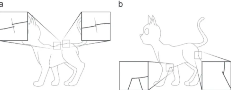
Our method builds a 3D model from a single 2D sketch. This involves the following steps, which are also summarized inFig. 1. We start from a sagittal-view vectorized sketch of an animal in the (x,y) plane. The hand-drawn input sketch is transformed into a set of parametric curves using a vectorization algorithm such as the one proposed by Noris et al. [18]. These algorithms are relatively robust to noise and provide the smooth curves we seek. What the user must really pay attention to is the correctness of the input hand-drawn sketch topology, i.e., the provision of contin-uous closed contours that do not have spurious crossings with other contours.Fig. 2illustrates two failure cases, the first, in2(a), is due to an incorrectly closed contour and the second, in2(b), is due to an incomplete input.

The goal of the first step, detailed inSection 4, is to identify the strokes that correspond to the same structural part, such as an eye, leg, or body, and to infer any missing curves, i.e., perform contour completion, if the resulting contour is open. This is done in the following way: We build a counter-clock-wise oriented half-edge graph whose edges are in general bounded parametric curves (see

Fig. 1(a,b)). In this graph, we iteratively follow successive half-edges, and store cycles in a list (Fig. 1(c)). Each cycle is classified as being either an outer-sketch, island, border or other as explained in

Section 4.1and illustrated inFig. 1(d).

We then define as inner-edges those edges where both half-edges belong to the same cycle (the green half-edges inFig. 1(e)). These lists of inner-edges represent suggestive curves where two shape parts merge (such as a leg merging with the body). This implies the presence of hidden silhouettes or cusps[12]. Each suggestive curve has an open endpoint and a closed endpoing, which are depicted in red and blue, respectively, inFig. 1(e). The next step is to pair these suggestive curves and connect their extremities in order to infer new cycles representing the different structural parts of the animal (Fig. 1(f)). This is the topic ofSection 4.2.

The subsequent step, presented inSection 5, is the computation of a depth hierarchy for structural parts, based on the structural symmetry hypothesis. We first identify the main body part located in the saggital plane, i.e., the torso, and detect structural

Fig. 2. Two cases of failure: (a) Discontinuous sketch: a large discontinuity, as the one on the left, prevents the detection of the main body part in the drawing. In that case our algorithm fails from its first steps. A small gap in the sketch, as on the left, is filtered and considered as a connection during our first step. The reconstruction will perform adequately. (b) Incomplete sketch: on the left, a structural part is missing in the sketch, here, the left inner-body silhouette of the front foreground leg. Our algorithm will not be able to detect the presence of a limb and the reconstruction of the legs will fail. On the right, both inner-body silhouettes of the rear foreground leg are drawn and the rear legs will therefore be adequately reconstructed.

symmetries around it such as pairs of ears or pairs of front legs, cf.

Section 5.1andFig. 1(g)). We then use the pieces of information we already gathered, e.g., island cycles, structural parts, chest, and symmetries, to define a depth hierarchy between structural parts, as detailed inSection 5.2andFig. 1(h).

This leads us to the last step, detailed in Section 6 which consists of the 3D reconstruction of the animal model. For each pair of limbs, only the one in the foreground of the drawing is considered during the reconstruction steps. The 3D reconstruction of the background limbs is added at the end of the process by symmetry. We choose implicit surfaces to represent shape parts, in order to benefit from their blending capabilities. We first compute the medial axis[19]of each structural part (Fig. 1(i)). Medial axes are then filtered and specifically simplified in order to be used as skeletons for 3D implicit surface modeling (Section6.1andFig. 1

(j). Among the variety of existing implicit models, we use scale invariant integral surfaces (SCALIS)[20]to accurately reconstruct shape parts (Section6.2).Fig. 1(j)) shows the 3D reconstruction of each structural shape part in isolation. Structural parts without symmetries are placed in the sagittal plane of the model. The depth of the foreground structural parts is computed using the thickness of their 3D reconstruction and the thickness of the part to which it is connected in the sagittal plane (Section6.3andFig. 1

(k)). Symmetric background parts are then added to provide the final 3D model (Fig. 1(l)). The final shape is obtained using a simple sum to blend the fields from the different implicit primitives.

The next sections give a detailed presentation of our solutions at each stage of this process.

4. Structural parts identification and completion

4.1. Representing the sketch as a set of cycles

The first step is to decompose the curves of the sketch into a set of cycles. This decomposition is a preliminary step towards identifying the different parts of the animal drawn in the sketch. In particular, this step is required for the hidden contour computa-tion and the contour closure, as described inSection 5.

The input data is a hand-drawn sketch composed of a set of non-crossing curves that are connected to each other (seeFig. 1

(a)). Each of these curves is represented by a pair of directed half-edges1 _{of opposite direction (see Fig. 1(b)). The curves of the}

sketch are then represented using a graph whose edges are the half-edges of the curves and whose nodes are the points at which the curves are connected to each other. Next, we decompose this graph into a set of cycles.

Formally, a cycle is defined as a closed sequence of connected half-edges; each half-edge shares its endpoints with at least two other half-edges. We require the half-edges that compose a cycle not to cross each other; we also require the cycles to be topolo-gically equivalent to a disk. Therefore, a cycle divides the sketch into an “interior” region and an “exterior” region. In order to define the interior of a cycle, cycles and their associated half-edges are given a direction which is either clockwise or counter-clock-wise; the interior of the region bounded by a cycle lies on the left side of the directed half-edges that compose this cycle.

The first cycle that we identify is the one which is composed of the half-edges located along the outer boundary of the sketch. This cycle is oriented clockwise and is unbounded; it corresponds to the outer region of the sketch. We name this the outer sketch cycle. Next, we identify the border cycles which are cycles that

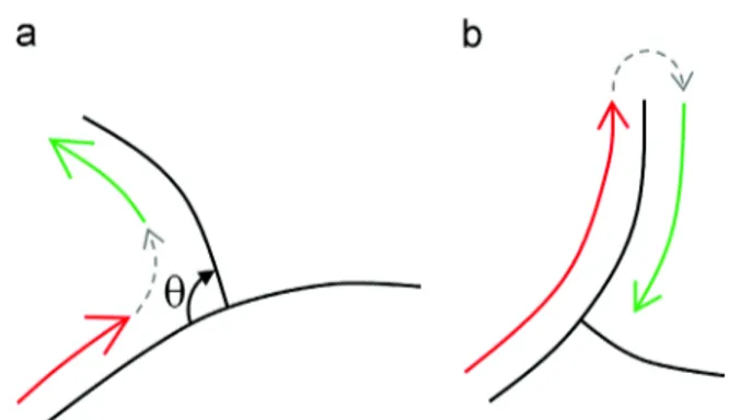
have one or several half-edges belonging to the outer boundary of the sketch. All of these cycles are oriented in a counter-clockwise fashion. The process to construct a border cycle is as follows: we first select a half edge which is located along the outer boundary of the sketch and which has not yet been associated to a cycle. We next find its endpoint by following its direction and select the next half-edge. This next half-edge is chosen such that its direction is the same as the previous half-edge and the clock-wise oriented angle between the two half-edges is the smallest possible, as illustrated in Fig. 3. The process of finding the next half-edge is iterated until we reach the first half-edge.

Finally, we identify the island cycles; island cycles are single half-edges that correspond to a closed curve with no self-intersection and which are not connected to any other curves of the sketch. These island cycles are also oriented counter-clockwise, meaning that they do not represent a hole but rather a surface feature of the animal (such as the eye of cat model shown inFig. 1). After processing all the cycles, there may remain some cycles that could not be classified as any of the three types (outer sketch cycles, border cycles and island cycles); we mark these cycles as others.

4.2. Contour completion

The goal is now to convert the set of cycles into closed contours associated to each structural part of the shape.

Once the graph cycles are classified as described above, we use the hypothesis that structural parts have at least one edge in contact with the outer part of the sketch, and consider only the border cycles. In these cycles, we extract the sets of neighbor embedded edges, i.e. edges whose half-edges both belong to the same cycle, and then annotate these as being suggestive curves. Each set is an open path in the graph with one extremity connected to the rest of the graph, i.e., a closed extremity, and one extremity without any connection, i.e., an open extremity (see

Fig. 1(e)). As we focus on organic models, the suggestive curves come from the drawing of the silhouette of structural parts that stop where the limb smoothly merges with the part of the shape over which they are drawn (for instance the cat legs over the body in Fig. 1). We require the user to provide two suggestive curves clearly delimiting each merging limb.

Parts need to be individually closed to be identified and reconstructed. To do so, we compute a set of cubic Bézier curves linking open extremities and closed extremities pairwise with a C1

continuous connection with the edge curves while minimizing the normalized sum of the curvature variations (“Gestalt principles”):

E ¼1 l∑i ki þ 1# kidl where ki¼J _ ci$c€iJ J _ci3J ; ! ! ! ! ! ! ! ! ! ! ð1Þ

Here, l is the curve length, kiis the curvature of the curve at

sample point i, _ci is the curve first derivative, and €ci is the second

derivative at parameter value ui.

The sum of curvature variations, lE, is used as the energy associated with the curve. For curves connecting closed extremi-ties, these energies are denoted Ecand for those connecting open

extremities they are denoted Eo. We then compute two energies Ei

ði ¼ 0; 1Þ for each pair of suggestive curves, one for each way the closed extremities can be connected (dashed curves inFig. 4(a,b)). These energies are computed as follows:

Ei¼ pi0:pi1

" #

Eoþ Eic

" #

; ð2Þ

where Eci is the energy associated to the curve connecting closed

extremities (i¼0 for the closure illustrated inFig. 4(a) and i¼ 1 for the one illustrated inFig. 4(b)), p0i and p1i are the probabilities that

the curve is correctly connected at each extremity respectively. These probabilities are computed as the ratio pi

j¼ min

α

ij=

β

j; 1

" #

1_{Note that each graph edge geometrically correspond to a full curve of the} sketch.

(j¼ 0,1) in which angles

α

0

0 and

β

0are illustrated in Fig. 4(c). All

other angles are defined in a symmetric fashion. The best-matching pair of suggestive contours is then chosen as the pair having the minimal sum of energies.

Once the suggestive contours are paired and closed, we define their set of half-edges and derive the new cycles. In these cycles, no edge is embedded in the defined part (i.e. no edge has both half-edges in the same cycle). Together with the remaining border cycles and the island cycles, this gives us the set of the animal structural parts drawn in the sketch.

The minimization of curvature variations is known to provide plausible results when completing organic curves. The selected completion curves linking open and closed extremities does not, in general, intersect other contours. However, if this should occur, it will not be expected as it does not faithfully correspond to the intent of the input sketch, although it does not compromise the rest of the reconstruction. If necessary, the user can correct the completion by editing the extremities.

5. Depth hierarchy of structural parts

5.1. Body and symmetrical parts

In order to assign appropriate depth values, we create a graph that represents the desired depth relations. This begins with the

choice of a reference part as the root node of the graph, for which it is natural to use the body or torso. For some animals, this main body part may be smaller than the limbs. As such, we did not find a robust method to automatically label this in the input sketch. Instead, we request the user to select it or to draw the sketch so as to locate it in the center of the drawing canvas. Once labeled, this part defines the node of reference for the graph. The method described below automatically locates the remaining structural parts with respect to the body, in terms of their relative depth. We begin by detecting the sketch strokes that correspond to pairs of symmetric parts, as explained next.

We already know the parts, Fi, that should be located in front of

the body and thus that may have a symmetrical part in the background. These are defined by the open contours with sugges-tive curves we just completed at the previous step. The goal is now to identify the strokes from the sketch corresponding to Bi, the

structurally symmetric part with respect to Fi, but located in the

background. Indeed, Bishould not be processed any further, since

we are going to use symmetric geometry to create the background limbs. In practice, Bimay be composed of several distinct cycles,

since it is partly occluded. We use a propagation method for fully selecting it, as we now describe.

We initialize Biwith all cycles not belonging to the shape part

under Fi, but that share an edge with Fi. We then compute the

medial axis of Fias described inSection 6. Let us denote as p0the

medial axis extremity corresponding to the suggestive silhouette we closed (see Fig. 5). We then denote as p1 the middle of the

closed extremities of the suggestive curves and then define

v0¼ p1# p0. Starting from both closed extremities, we march along

both sides (one clock-wise and the other counter-clock wise) of the cycle of the structural part which is located under Fiin the

sketch, as long as the opposite half-edge belongs to the outside sketch. If we meet an opposite half-edge belonging to a border cycle, we get both extremities of the shared edge and we compute their middle point p2. We define v1¼ p2# p0 and compute the

angle

α

¼ jvd0; v1j. If

α

o

π

=4 we consider that this cycle potentially belongs to Bi, since the angle formed by two symmetrical parts is

unlikely to be larger than this value in usual standing poses. Note that this criterion could be relaxed to handle a larger set of poses. We stop when the half-edge we reach is an occluded edge, i.e., when we meet the next foreground part. If selected on multiple occasions, a potentially symmetric cycle is assigned to the Bifor

which the angle

α

with Fiis minimal. The results of this selection

Fig. 3. Selecting the next half-edge. In (a), the selection of the next half-edge (shown in green) for T-junctions is chosen such that the angle between the next half-edge and the preceding one (shown in red) is the smallest possible. In (b), the selection of the next half-edge for cusps. (For interpretation of the references to color in this figure caption, the reader is referred to the web version of this paper.)

β0

α0 0

Fig. 4. (a) and (b): Illustration of the two possible completions of a pair of closed extremities. (c) Close-up on a closed extremity illustrating the two angles α0

0and β0 used in the computation of the probability p0

0.

p

₀

p

₁

p

₂

v

₀

v

₁

α

Fig. 5. Identification of the cycles belonging to the shape part at the background that is structurally symmetrical to a foreground limb.

process are depicted inFig. 1(g), where pairs of symmetric parts are depicted using the same colors.

5.2. Graph construction

In order to support the 3D reconstruction of the model, we build a graph whose nodes are the structural parts (and their associated cycle) and whose edges represent the relations over,

under, adjacent or over-in with respect to the main body.

Fore-ground parts are defined as lying over the part they have been separated from. Symmetric counterparts are located under the part that their foreground is over. All remaining border parts that have not been designated as part of a symmetric pair are defined as being adjacent to parts with which they share an edge. Islands are assigned to the graph by first using a simple 2D ray-cast in the sketch plane in order to identify the part within which the island lies. The island cycles are over and inside a structural part, and this part is also then defined as being under the island. Each edge is further tagged with additional information, such as the presence of suggestive curves, which help determine if the region being over a particular part is an island or a limb.

6. 3D Reconstruction

6.1. Medial-axis computation and simplification

Animals have the convenient property that their shape is naturally approximated as a set of generalized cylinders. A gen-eralized cylinder is a surface obtained by moving a circle of varying radius along a 3D arbitrary curve. An advantage of generalized cylinders is that their skeleton and associated radii are easily determined from their projected image. Given a 2D simple closed curve C, the skeleton and the associated radii of the generalized cylinder whose orthogonal projection matches C are obtained by computing the medial axis and the associated radius function of the curve C.

We start the 3D reconstruction step by reconstructing each structural part independently. The parts which were detected as being symmetric to foreground parts are not considered. The contour curve of each part is first sampled so as to obtain a polygonal curve. We then compute the medial axis transform of each of the polygonal curves using the Fortune's sweep-line algorithm[19]. The medial axes usually contain many branches because of the noise in the polygonal curves. We use the Scale-Axis Transform method by Giesen et al. [21] to remove these branches. In our experiments, the scale factor of the Scale Axis Transform has been set to 1.2.

The last step is to simplify the medial axis; the purpose of this simplification is to lower the computation time for generating the surface of the reconstructed animal. We have implemented a modified version of the Douglas–Peucker algorithm[22]which is a method to reduce the number of points of polygonal curves. A cost function is defined for each point, which is the maximum distance between the original curve and the curve after removing the point. Points are removed iteratively in increasing order of their cost. The algorithm stops when the cost of the point to remove is above a user threshold.Fig. 6(b) illustrates the result of the cat skeletons simplification.

The Douglas–Peucker algorithm has been modified to take into account the radii of the medial axis. This modification consists of a new cost function. Let C be a polygonal curve and pA, pB, pC be

three neighboring points of the medial axis of C. If the point pBis

removed, the two segments pApB and pBpC are replaced with the

segment pApC(seeFig. 7). Similarly, the curve corresponding to the

medial axis is simplified; two of its segments are removed. The

new cost function is defined as the maximum distance d between the original curve and the curve after the simplification of the medial axis.

6.2. Surface reconstruction of the shape components

Once the skeletons of all the shape components have been computed, the next step is to reconstruct the 3D surface of these shape components. We have implemented the SCALe-invariant Integral Surfaces (SCALIS) method proposed by Zanni et al. [20]. This method generates an implicit surface using a skeleton and its radius function. In Zanni's method, the scalar field is computed with the Homothetic Polynomial kernel of degree 8. In our method, we have implemented the kernel of degree 6 instead of degree 8. Although the quality of the reconstructed surface is slightly lower, the computation time is much smaller, and allows for surface reconstruction at near-interactive rates. The result is a set of implicit surfaces, one for each shape component (seeFig. 1

(k)).

6.3. Placement and embedding of the shape components

The last step of the surface reconstruction is to assemble the implicit surfaces to generate the 3D shape of the animal. At this stage, the skeletons of the implicit surfaces are all located in the same plane which is the sketching plane. The goal is to place these implicit surfaces so that their depth order complies with that of the sketch; the shape components that are drawn in the sketch foreground should be placed in front of the sketching plane and those drawn in the sketch background should be placed behind the sketching plane. We make use of the depth graph that has been previously computed (see Section 5.2).

We start by placing the implicit surface corresponding to the main body component in the sketching plane. Other implicit surfaces are sequentially placed as follows. Using the depth graph, we find a shape component that has not yet been placed and which is adjacent to a shape component which has already been placed. Using the depth order between these two shape compo-nents, we compute the depth position of the one to be placed.

Let IAand IBbe two implicit surfaces, with IAbeing in front of IB.

The depth coordinates of IBhave been already computed; those of

IAhave to be computed. Let pAand rAbe the skeleton extremity of

the implicit surface IAand its radius respectively. We first compute

pA;0the orthogonal projection of pAonto IB. Next, we compute N%%!A;0,

the surface normal of the implicit surface IB at the point pA;0.

Finally, we compute p_A;1 such that Jp%%%%!A;1pA;0J is equal to rAand

such that the two vectors N%%!_A;0 and p%%%%! are parallel and have_A;1pA;0

same direction (seeFig. 8(a)). The depth coordinate dA;1 of pA;1 is

then used as the depth coordinate of all the points of the skeleton of IA(seeFig. 8(b)).

Once the depth coordinates of all the implicit surfaces have been computed, the 3D shape of the animal is then generated by blending these implicit surfaces using the well-known Ricci blending operator.

7. Results and discussion

We implement our method as a Maya plugin, enabling us to use the existing sketching interface of Maya to design the vectorized sketches we need as input. Processing the 2D sketches into 3D models is then a fully automatic process.

The teaser image andFigs. 9–12show a set of results from our method. They validate the fact that our method is able to generate plausible rough shapes for various animals from a single sketch. Note that since we only used a structural symmetry hypothesis

around the sagittal plane, our animal models may have an arbitrary number of protruding subparts such as limbs, ears (interpreted as volumes) or horns. Moreover, our choice of scale invariant implicit surfaces (SCALIS) as the 3D representation enables us to capture both the smoothness of organic shapes and the singularities that may come from the sketch, such as at the tip of the cat ears.

Pairs of limbs are reconstructed symmetrically, but the user can manually adjust the pose in 1 to 3 minutes by deforming the geometric skeleton (seeFig. 1(i) the geometric skeleton of the cat model). Background limbs can be positioned in sketch pose as in

Fig. 12(c), or the model can be globally deformed as in Fig. 12

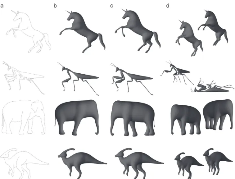
(mantis-d). InFig. 12(elephant), the ears are not reconstructed as they do not represent any of the different cycles considered in the sketch for our reconstruction (as explained inSection 4.1).

The results have been produced on an Intel Core i7 3770 K computer, and the code is compiled with ICC 15.0 in release mode. For all our examples, the full sketch-processing and 3D modeling process run in less than one second. This makes the method applicable within an interactive sketching software tool. More precisely, the computational time for the giraffe is 0.35 s, for the gazelle is 0.30 s and for the cat 0.37 s.

To further validate our system we performed a preliminary user study with 4 different users ranging from beginners to a

professional computer artist. Their sketches and resulting models are shown in Fig. 13. They all found the concept of suggestive curves to delimit the limbs quite easy to understand. When asked how well the 3D model met their expectations, on a scale from 1– 9, they gave a score of 7. The time spent to create the input drawings using the Pencil Curve Tool in Autodesk Maya was less than 2 minutes for all the drawings, with the exception of the rabbit, which took 10 minutes to draw.

Limitations: Our method has a number of remaining limitations.

First, we are limited in the range of sketches we are able to handle:

)

The sketch cannot include adjacent internal parts (islands in our terminology) such as if the cat had two adjacent eyes. Otherwise, the classification algorithm will fail;

)

A shape part cannot self-overlap in the sketch (such as an animal tail looping and self-occluding itself), nor overlap any other shape part (such as a tail occluding the animals body). Our completion algorithm does not handle these cases. Note that we partly avoid this occlusion problem by using symmetry when creating the limbs, but developing a more general solution would be desirable.

)

Drawing pairs of suggestive contours is mandatory when two shape parts blend (such as at the top of a front leg, where it blends with the body), and these contours should be such that our completion algorithm keeps the reconstructed part of the contour inside the main body-shape. Although this holds true in most cases, we currently offer no guarantees regarding this point.

A second family of limitations concerns the 3D shape we output:

)

All the shape parts we create have a planar medial axis, which we locate in a vertical plane. Although this works quite well for the legs, this method needs to be improved for parts such as

Fig. 6. Medial axis computation and simplication. In (a), the medial axes of the sketch components computed using Fortune's sweep-line algorithm[19]. In (b), the skeletons after removing the branches using the Scale-Axis Transform[21]and after simplifying the medial axes using the Douglas–Peucker algorithm[22].

A

p

B

p

C

p

d

A

p

C

p

Fig. 7. Medial axis simplification. In (a), the polygonal curve (depicted in black) and its medial axis (depicted in red) before the simplification. In (b), the medial axis has been simplified by removing the point pB. The result is new polygonal curve with fewer segments. The cost value of removing the point pBis d; it is the maximum distance between the original curve (depicted in light gray) and the curve after the simplification. (For interpretation of the references to color in this figure caption, the reader is referred to the web version of this paper.)

the ears or the horns, which should preferably be oriented to lie in a direction that is normal to the surface.

)

We only use segment skeletons for generating the implicit shapes, as opposed to surface skeletons, which restricts our construction to generalized cylinders. This prevents us from capturing the flat surfaces that one can readily observe on the

flanks of many animals, or flat features such as elephant ears that cannot be reconstructed with our approach (seeFig. 12).

)

We reconstruct pairs of limbs using symmetric poses. Auto-matically fitting the reconstructed background parts is non-trivial since we do not reconstruct a rigging skeleton and most of the drawing of the background limbs is missing. Performing this fitting remains a challenging open problem on its own.

8. Conclusions and future work

We have presented the first method, to the best of our knowl-edge, for creating 3D animal models from a single sagittal-view sketch. Our method handles complex sketches with open curves, closed curves, and T-junctions. Once the main body part is selected, the method is fully automatic for reconstructing a symmetric version of the 3D shape. The reconstructed shape is

I

p

_A,0

p

_A,1

I

p

N

_A,0

r

Sketching

plane

d

_A,1

d

A,1

Sketching

plane

Fig. 8. Computation of the depth coordinates of the implicit surface IA. In (a), the depth coordinate dA;1of the skeleton extremity pAis computed. In (b), the skeleton (depicted in red) of IAis translated to the depth coordinate dA;1. (For interpretation of the references to color in this figure caption, the reader is referred to the web version of this paper.)

Fig. 9. Different views of the 3D reconstruction of the cat sketched in the top-left.

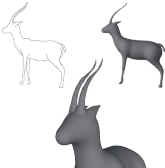
Fig. 10. Different views of the 3D reconstruction of the gazelle sketched in the top-left.

Fig. 11. Reconstruction of a dog and a penguin. (a) The input vectorial sketch, (b) the automatically generated result and (c) different view of the reconstructed model.

inferred using only two hypotheses: shape smoothness, except at singular points appearing on the sketch contour; and structural symmetry. The resulting 3D model can then be posed using standard software or by directly manipulating its skeleton.

In future work, we would like to address some of the limita-tions we listed. In particular, we are in the process of extending our stroke classification and completion method to more general

families of sketches. Being able to convert any sketch to the vector graphic complexes proposed in[23]would be an excellent inter-mediate step for our application. In addition, exploiting the 2D detection of partial symmetries in the cycles, using techniques such as the one by Mitra et al.[24], may be a promising direction of investigation for improving the pairing stage of our approach. This could also help for handling more complex inputs such as

Fig. 12. Reconstruction of a mantis, an elephant and a dinosaur. (a) The input vectorial sketch, (b) the automatically generated result, (c) the model with the foreground limbs manually adjusted to the sketch and (d) different views of the reconstructed models. The mantis is shown with different poses in (d).

sketches in arbitrary views. A last caveat is that the technique we currently use is not able to reconstruct large flat parts such as wings. A direction is to use more complex skeletons including surface parts as was previously done in the context of reconstruc-tion with convolureconstruc-tion surfaces [25].

Acknowledgments

We also thank the anonymous reviewers for their useful comments and suggestions, as well as Cédric ZANNI for sharing his implementation of SCALIS. This work was funded by the advanced grant EXPRESSIVE from the European Research Council (ERC-2011-ADG_20110209) and by the project IM&M (ANR-11-JS02-007).

References

[1] Cook MT, Agah A. A survey of sketch-based 3-d modeling techniques. Interact Comput 2009;21(3):201–11.

[2] Olsen L, Samavati FF, Sousa MC, Jorge JA. Technical section: sketch-based modeling: a survey. Comput Graph 2009;33(1):85–103.

[3] Igarashi T, Matsuoka S, Tanaka H. Teddy: a sketching interface for 3d freeform design. In: Proceedings of the twenty-sixth annual conference on computer graphics and interactive techniques, SIGGRAPH '99, 1999, p. 409–16. [4] Gingold Y, Igarashi T, Zorin D. Structured annotations for 2d-to-3d modeling.

In: ACM SIGGRAPH Asia 2009 papers, SIGGRAPH Asia '09. ACM, New York, NY, USA, 2009, p. 148:1–:9.

[5] Schmidt R, Wyvill B, Sousa MC, Jorge JA. Shapeshop: sketch-based solid modeling with blobtrees. In: ACM SIGGRAPH 2006 courses, SIGGRAPH '06. ACM, New York, NY, USA, 2006.

[6] Bernhardt A, Pihuit A, Cani MP, Barthe L. Matisse: painting 2d regions for modeling free-form shapes, in: Proceedings of the fifth eurographics con-ference on sketch-based interfaces and modeling, SBM'08, Eurographics Association, Aire-la-Ville, Switzerland, Switzerland, 2008. p. 57–64. [7] Kraevoy V, Sheffer A, van de Panne M. Modeling from contour drawings, in:

Proceedings of the sixth eurographics symposium on sketch-based interfaces and modeling, SBIM '09, ACM, New York, NY, USA, 2009. p. 37–44. [8] Fonseca MJ, Ferreira A, Jorge JA. Sketch-based retrieval of complex drawings

using hierarchical topology and geometry. Comput Aided Des 2009;41 (12):1067–81.

[9] Rivers A, Durand F, Igarashi T. 3d modeling with silhouettes. ACM Transactions on Graphics (SIGGRAPH 2010) 29 (4).

[10] Schmidt R, Khan A, Singh K, Kurtenbach G. Analytic drawing of 3d scaffolds. proceedings of ACM Transactions on Graphics (SIGGRAPH ASIA 2009) 28(5). [11] B. Xu, W. Chang, A. Sheffer, A. Bousseau, J. McCrae, K. Singh, True2form: 3d

curve networks from 2d sketches via selective regularization, Transactions on Graphics (Proc. SIGGRAPH 2014) 33(4).

[12] Karpenko OA, Hughes JF. Smoothsketch: 3d free-form shapes from complex sketches, in: ACM SIGGRAPH 2006 Papers, SIGGRAPH ’06. ACM, New York, NY, USA, 2006. p. 589–98.

[13] Ijiri T, Owada S, Igarashi T. Seamless integration of initial sketching and subsequent detail editing in flower modeling. Comput Graph Forum (Euro-graphics 2006) 2006;25(3):617–24.

[14] Turquin E, Wither J, Boissieux L, Cani M-P, Hughes JF. A sketch-based interface for clothing virtual characters. IEEE Comput Graph Appl 2007;27(1):72–81. [15] Wither J, Boudon F, Cani M-P, Godin C. Structure from silhouettes: a new

paradigm for fast sketch-based design of trees. Comput Graph Forum 2009;28 (2):541–50 special issue: Eurographics 2009.

[16] Pihuit A, Cani M-P, Palombi O. Sketch-based modeling of vascular systems: a first step towards interactive teaching of anatomy. In: Proceedings of the seventh sketch-based interfaces and modeling symposium, SBIM '10, Euro-graphics Association, Aire-la-Ville, Switzerland, Switzerland, 2010. p. 151–8. [17] Cordier F, Seo H, Park J, Noh JY. Sketching of mirror-symmetric shapes. IEEE

Trans Vis Comput Graph 2011;17(11):1650–62.

[18] Noris G, Hornung A, Sumner RW, Simmons M, Gross M. Topology-driven vectorization of clean line drawings. ACM Trans Graph 2013;32(1):4:1–4:11. [19] Fortune S. A sweepline algorithm for voronoi diagrams. In: Proceedings of the

second annual symposium on computational geometry, SCG '86. ACM, New York, NY, USA; 1986. p. 313–22.

[20] Zanni C, Bernhardt A, Quiblier M, Cani M-P. SCALe-invariant integral surfaces. Comput Graph Forum 2013;32(8):219–32.

[21] Giesen J, Miklos B, Pauly M, Wormser C. The scale axis transform. In: Proceedings of the twenty-fifth annual symposium on computational geome-try, SCG '09, ACM; 2009. p. 106–15.

[22] Douglas DH, Peucker TK. Algorithms for the reduction of the number of points required to represent a digitized line or its caricature. Cartograph Int J Geogr Inf Geovis 1973;10(2):112–22.

[23] Dalstein B, Ronfard R, van de Panne M. Vector graphics complexes. ACM Trans Graph 2014;33(4):133.

[24] Mitra NJ, Guibas L, Pauly M. Partial and approximate symmetry detection for 3d geometry. ACM Trans Graph (SIGGRAPH) 2006;25(3):560–8.

[25] Alexe A, Barthe L, Cani M, Gaildrat V. Shape modelling by sketching using convolution surfaces. In: Pacific graphics (Short Papers); 2005.