Science Arts & Métiers (SAM)
is an open access repository that collects the work of Arts et Métiers Institute of Technology researchers and makes it freely available over the web where possible.
This is an author-deposited version published in: https://sam.ensam.eu Handle ID: .http://hdl.handle.net/10985/9221
To cite this version :
Nazih MECHBAL, Michel VERGÉ, Gérard COFFIGNAL, Manickam GANAPATHI - Application of a Combined Active Control and Fault Detection Scheme to an Active Composite Flexible
Structure. - Mechatronics - Vol. 16, n°3-4, p.1993-208 - 2006
Any correspondence concerning this service should be sent to the repository Administrator : archiveouverte@ensam.eu
Application of a Combined Active Control
and Fault Detection Scheme to an Active
Composite Flexible Structure.
N. Mechbal
a*, M. Vergé
a, G. Coffignal
a, Ganapathi
b aLaboratoire de Mécanique des Structures et des Procédés (LMSP – UMR, CNRS), École Nationale Supérieure des Arts et Métiers (ENSAM), 151 Boulevard de l'Hôpital, Paris, France.
b
Institute of Armament Technology, Girinagar, Pune, 411025, India.
Abstract
In this paper, the problem of increasing reliability of active control procedure is considered. Indeed, a design method of rejection perturbation in presence of potentially faults, on a flexible structure with integrated piezo-ceramics, is presented. The piezo-ceramics are used as actuators and sensors. A single unit based solution, which handles both control action and fault diagnosis is proposed. The algorithm uses H∞ optimization techniques. A full order model of the structure is first obtained via both finite-element (FE) approach and identification procedure. This model is then reduced in order to be used in our robust approach. By a suitable choice of weightings functions, the provided method is able to reject disturbance robustly and to estimate occurred faults. The case of sensors and actuators faults is discussed. The choice of weightings for diagnosis and control systems is also tackled. Finally, the effectiveness of this integrated method is confirmed by both simulation and experimental results.
Keywords: Active control, Fault detection, H∞ optimization, Composite beam, Finite-Element model, Piezo-ceramics.
*
Corresponding author.
Tel. +33-1-44-24-64-58; Fax: +33-1-45-86-21-18 E-mail address: Nazih.Mechbal@paris.ensam.paris
1. INTRODUCTION
In many industrial and spatial applications, noise and vibration are important problems. The conventional method of treatment is to use passive damping techniques. However, these techniques are primarily effective at a limited band of frequencies. In the past decade, active control of vibrations has emerged as a viable technology to bridge this low-frequency technology gap. Recent developments have been propelled by the rapid technology growth in practical digital signal processing and by the use of promising smart materials with adaptable properties such as ceramics. Indeed, piezoelectric devices, as in particular PZT piezo-patches, seem very attractive to carry out the function of sensor and actuator. The aim of reducing the vibrations may now be reached with a lower increase of weight.
The smart structure obtained is able to react to external perturbations. It is more efficient than passive absorption ([1]). But it is also more sensitive to the failure of any element (e.g. actuators, sensors or onboard electronics), which can destabilize the control law and cause severe damages to the structure. In fact, due to wear of mechanical and electrical components piezo-ceramics might fail in more or less critical way. As a consequence, procedure of fault detection and isolation (FDI) can be necessary to ensure a reliable and safe operating.
The theory of FDI has known a great interest during these last three decades ([2], [3]).The general concept of analytic FDI procedure is to compare the actual behavior of the monitored plant to that expected on the basis of a mathematical plant model. Plant models, however, are generally incomplete and inaccurate. Moreover, exogenous inputs, noises and modeling errors can either cause excessive false alarms and missed detection, or make it difficult to detect failures. Hence, any robust FDI procedure must be able to separate the effect of perturbation from the effect of failures.
Furthermore, the modeling of a physical system for feedback control invariably involves a trade-off between the simplicity of the model and its accuracy in matching the behavior of the physical system. In active control and because of the highly flexibility of the class of systems under study, the goal is to design a feedback controller which increases the system damping. Moreover, these systems present many modes but the controller designed is usually based only on few of them. This can provoke the apparition of spillover phenomena and hence lost of control ([4]). Beside this, stiffness and natural frequencies can only be approximately estimated. Hence, it is desirable that the closed-loop be robustly stable to variation of these parameters and to spillover. As a consequence, it is necessary to use robust control law and robust fault detection algorithms ([5]).
Many effective methods have been proposed to solve this problem. But most of them are based on generating fault detector independently from the control law ([6]). In this paper, we propose to apply to a composite flexible structure, a single algorithm that handle both the required robust active control law, as well as detecting fault occurrence in active elements. This dual problem is formulated as an H∞ design problem by using a standard system setup. Both for control law and for FDI, H∞ optimization techniques have been intensively used to generate robust controller ([7]-[10]) and robust filter detectors ([11], [12]).
Combined approach has been studied by [13], [14] and [15]. In this paper, we use the algorithm developed by Stoustrup and al. ([15]-[17]). This algorithm is based on frequency domain H∞ formulation that makes weight selection more straightforward specially to improve the robustness to neglected dynamics introduced by the model reduction. This - 2 -
algorithm is based on a kind of separation principle, which respects the fundamental trade-off between diagnosis and control systems. Moreover, the use of a combined module can be beneficial in terms of implementation and reliability.
Moreover, as in [18] and [19], here, the problem of robust detection is also reformulated in a problem of optimal robust estimation, where now the unmeasured signal to be estimate is the input fault signal. Indeed, in this case, diagnostic of faults is straightforward rather using a common two main stages approaches: robust residual generation and robust residual evaluation.
The flexible structure under study is a composite beam with piezoelectric patches as sensors and actuators. Hence, to perform classical linear dynamical analyses we use Nastran software to realize the finite-element (FE) model. However, this software does not contain any specific elements dealing with the piezoelectric coupling (electrical-mechanical) problem. Hence, we have elaborated an original strategy of simulation, which consists in exploiting the analogy between thermal and piezoelectric equations. The FE model obtained is then compared (in order to update it) to an actual model obtained by experimental identification.
The main contribution of this paper is to show how H∞ optimization can be satisfactorily employed for control and fault estimation of flexible structure equipped with PZT actuators and sensors. The effectiveness of this integrated method is confirmed by both simulation and experimental results.
The paper is organized as follows. After a description of the active structure in section 2 the FE model and simulations are presented in section 3. In section 4, an experimental identification of the actual physical process is performed and matched with the FE model. In section 5, the combined feedback controller and fault estimator is formulated as an H∞ design problem. Simulation and experimental results on the composite structure are given in section 6. A conclusion is drawn in section 7.
2. EXPERIMENTAL SETUP
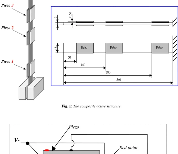
The structure is made of a composite beam with 3 pairs of piezoelectric ceramics bounded symmetrically to the beam and covered by very thin electrodes on their top and bottom sides. The beam of dimension 360 ×18×3mm, is constituted of two external thin plates (thickness 0.5mm) between which is inserted a composite filling (thickness: 2mm). The structure is illustrated in Fig. 1.
The actuators and sensors are PZ29 piezoelectric ceramics type with dimension 49×24.5×0.51mm. PZT (Lead Zirconate Titanate) is a very stiff and transversely isotropic material with large piezoelectric coefficients. They are positioned parallel to the mid plate surface and polarized in a way that permits sensing or supplying pure bending motion (see Fig. 2). The composite element is realized with pre-impregnated plies of composite material of reference 07628 ES15. The beam is in vertical position (see Fig. 1) and the piezoelectric are numbered. Their position has been determined by FE approach ([20]).
Piezo 1 Piezo Piezo 2 3
Piézo Piézo Piézo
18 50 140 280 360 2 0,51
Fig. 1: The composite active structure
Red point Piezo
V-
V+
Composite
Fig. 2: Piezoelectric ceramic bounded to the beam and its polarization
The setup is completed by a control loop: charge amplifiers (Kistler© amplifier) for the conditioning of measured signals, tension amplifiers (Trech© amplifier) for the actuators and a specialized Dspace© card performing the real-time measurements and control.
3. FE MODELING AND NASTRAN SIMULATIONS
The FE method is a powerful approach to numerical analysis. It permits to model mechanical structures with arbitrary geometry and material properties. With this approach and without losing generality, the equation of motion of a linear flexible structure can be written as Q q K q C q M &&+ &+ =
where M, C and K are respectively the mass, damping and stiffness matrix of the solid structure (including active elements). Q is the external generalized force vector. q is the
nodal displacement vector. To predict the dynamic behaviour of the whole structure, the embedded piezoelectric active devices must be introduced in the last equation to set up Q . 3.1. Formulation of piezoelectric elements
In the following model formulation, we assume that the piezoelectric patches are perfectly bounded to the plate and the elastic field in such materials is coupled with the electric field.
Finite element equations for piezoelectric materials have already been formulated in many papers (for example, [20]). The linear constitutive relations for the direct and the inverse piezoelectric effects can be written as:
E d SE − T = σ
ε
E d D= σ +εσwhere the superscript T denotes a matrix transpose,
ε
is the vector of strain tensor components, σ is the vector of stress tensor components, D is the electric displacement vector, E is the electric field vector, S is the elastic flexibility matrix evaluated at constant EE, d is the piezoelectric coupling matrix and εσ is the dielectric matrix at constant stress. These equations can also be written in a more suitable way as,
E e CE − T =
ε
σ E e D=ε
+εεwhere εε is the dielectric matrix at constant strain and C is the elastic stiffness matrix E
evaluated at constant E.
3.2. State representation and model reduction
Piezo-ceramics are discretized by mean of plate elements in order to model their mass and rigidity. The coupling is then introduced in the finite-element model that leads to the following equation ([5]). ) (t u Q Q Q a ext + = where ext
Q represents external mechanical strength and Qa. represents actuator's effects. u
is the input voltage. By duality, the characterization of the piezoelectric direct effect leads to a relation between the output voltage and a function of the vector of mechanical nodal displacement: ) (t u ) (t y ) ( ) (t Q q t y = c
Now, using the previous finite element model and taking into account a disturbance input, with form ) (t d Q Q d ext =
the equation of the motion of the active flexible structure becomes, d Q u Q q K q C q M d a + = + + & &&
Defining the mode shape Φi and the angular frequency ωi of the i
th
mode as the solution of the following generalized eigen problem ([1], [5]):
i i
i M
KΦ =ω 2 Φ ,
there exist then N linearly such Φi where N is size of the differential system (usually N is very large). A reduction is done by projection of the nodal displacements on a truncated modal matrix. Let Φ be this modal matrix and g the vector of the associated generalized displacements defined by:
[
Φ1 Φn]
, n<<N ; q=Φ.g=
Φ L
After some substitution and left multiplying by Φ the equation of the motion can be T rewritten as: Q g k g c g m &&+ &+ =ΦT
where m, c and k are diagonal matrices provided C has convenient properties.
The most important stage in the reduction of order is the choice of the eigen modes kept in the reduced modal basis. Given the position of actuators and sensors, the modes are sorted regarding to their H∞ norms as described in [5]. By choosing now the state vector as
⎟⎟ ⎠ ⎞ ⎜⎜ ⎝ ⎛ = g g x & ω ,
we obtain a 2n order model that we turn into state space representation as
ζ ω ζ ω ω ⎥ ⎦ ⎤ ⎢ ⎣ ⎡ Φ + ⎥ ⎦ ⎤ ⎢ ⎣ ⎡ Φ + ⎥ ⎦ ⎤ ⎢ ⎣ ⎡ − − = d T n a T n i i i i n n Q u Q x diag diag diag x , 0 ,1 0 ,1 ) ( 2 ) ( ) ( 0 & y=
[
QcΦdiag(1/ωi) 01,n]
xFrom this state model we can then easily obtain the transfer functions of the process and the perturbation. In our application, for each transfer function, the first four modes were considered sufficient as it will be shown regarding to the efficiency of the controller.
3.3. Actuator simulation
The Nastran software does not contain any specific elements dealing with the piezoelectric coupling problem. To solve this problem, we have first exploited the analogy between thermal and piezoelectric equations. And then, we have used Nastran to perform classical linear dynamical analyze.
Hence, with this original approach a straightforward actuator simulation is possible. As a matter of fact, to formulate an actuator, we assume that the electrical field is constant through the thickness and perpendicular to the midsurface, and we use the following thermal equation:
th C C
ε
ε
σ
= − with(
T T0)
th =α − ε .Where α =
[
α1 α2 α3 0 0 0]
T, αi the coefficient of dilation in the direction i, the initial temperature and T the final temperature.0
T
We recall that the inverse piezoelectric effect is written as: E e CE − T =
ε
σ with[
]
T h V E = × 0 0 1 .Where h is the thickness of the piezoelectric ceramic (see Fig. 2). Matching the two equations, we obtain: E e C T th Eε =
Hence, using εth =CE −1eTE we have a direct analogy between the two couplings. Taking now and T0 =0 αi =α one can determine the parameters (α1,α2,α3,T ) allowing simulating the piezoelectric coupling. This leads to the following systems:
(
)
(
)
(
)
(
)
(
)
(
)
⎪ ⎪ ⎪ ⎩ ⎪ ⎪ ⎪ ⎨ ⎧ + + = + + = + + = ⇒ ⎪ ⎪ ⎪ ⎩ ⎪ ⎪ ⎪ ⎨ ⎧ = + + = + + = + + h e S e S e S h e S e S e S h e S e S e S T h V e S e S e S T h V e S e S e S T h V e S e S e S E E E E E E E E E E E E E E E E E E 1 1 1 33 13 31 22 31 12 2 33 13 31 22 31 12 2 33 13 31 12 31 11 1 3 33 33 31 13 31 12 2 33 13 31 22 31 12 1 33 13 31 12 31 11 α α α α α α Remarks:Because the piezoelectric materials are transversely isotropic leads to consider a thermal transversely isotropic behavior.
When we simulate an electrical excitation, we impose therefore a temperature on the surfaces of a piezoelectric pair that will induce a structure deformation. It is a linear problem taking into account the change of temperature but uncoupled in the sense that the temperature profile is imposed and does not evolve. Hence, we do not need thermal balance calculus.
3.4. Sensor simulation
A piezoelectric sensor can detect the strain when it is connected to a current amplifier. Indeed, when deformed, it accumulates an electric charge on their surface electrode. Hence, represents the image of the strain and it is given by ([20]):
) (t q ) (t q
∫
∫
+ − ∑ − − ∑ + + Γ+ Γ = 2 2 1 1 ) (t e n d e n d q ε εwhere and are respectively the upper and lower surfaces of the upper and lower electrodes. and are the normals to the upper and lower electrodes as shown in Fig. 2. In practice, we use a charge amplifier to measure . The output voltage is then given by:
+ Σ1 Σ− 2 + 1 n n2− ) (t q ) ( ) (t q t y =β
where β is an amplification coefficient.
Now, by using Nastran Reissler-Mindlin plate's theory associated with the finite-element method ([21]) applied in displacement to the Nastran CQUAD4 element, the output voltage
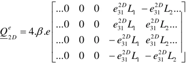
can be written in terms of the element displacement vectors ) (t y q as: e e T e D q Q t y( ) . 2 = where - 7 -
⎥ ⎥ ⎥ ⎥ ⎦ ⎤ ⎢ ⎢ ⎢ ⎢ ⎣ ⎡ − − − − = 2 2 31 2 2 31 2 2 31 2 2 31 1 2 31 1 2 31 1 2 31 1 2 31 2 ... ... ... 0 0 0 ... 0 0 0 ... 0 0 0 ... 0 0 0 ... . . 4 L e L e L e L e L e L e L e L e e Q D D D D D D D D e D β
and e and (or ) are respectively the thickness and the length of the i ceramic (see Fig. 1 and 2).
1
L L2
Finally, the last operation consists in gathering element matrices in order to set up the global model of the system. Following this approach, the output voltage of the charge amplifier is a linear combination of degrees of freedom (DOF). Consequently, by using the classical MPC (MultiPoint Constraint) of Nastran, this output voltage can be determined.
3.5. Simulations results
The global FE model obtained, allows the calculus of the modal deformation and eigen frequencies of the structure as well as the Bode diagrams of each transfer between a sensor and an actuator. For that, we suppose that the ceramics are perfectly pasted to the beam.
Hence, first vibration modes and frequencies obtained with this model are given in Tab. 1. We also have performed simulations that allow us to define the ceramics that are the most sensitive to one particular mode in the case where these modes are excited. This is very important in a control or in a perturbation rejection point of view.
4. EXPERIMENTAL IDENTIFICATION
Although methods and computers allow working with increasingly rich models, the modeling step constitutes a simplification quite rough of the physical reality. To validate the simplification hypotheses or to reduce errors by updating the model, it is necessary to make an experimental identification of the actual physical process ([22]).
We have thus, identified the structure by elaborating a model based on experimental Bode diagram. This model is then compared to the one obtained by FE simulations.
BEAM Actuator Amplifier Sensor Amplifier Oscilloscope Generator Treck Kist ler
Fig. 3: Experimental identification
Table 1
Vibration frequencies and modal deformation given by the FE model
Mode Frequency (Hz) Frequency (rad/s) Modal deformation
1 6,34 39,84 bending 2 43,51 273,38 bending 3 54,76 344,07 bending 4 127,47 800,92 bending 5 190,96 1199,84 torsion 6 257,77 1619,62 bending 7 370,18 2325,91 bending 8 478,93 3009,21 bending 9 661,11 4153,89 bending 10 695,98 4372,98 torsion
4.1. Experimental statements and first model
With the available actuators and sensors pasted on the beam, we have access to necessary information for its identification. We obtain experimental Bode diagrams (magnitude and phase) for each transfer between a sensor and an actuator (see Fig. 3). Indeed, as the beam is endowed with 3 sensors/actuators, it is therefore possible to define several couples of sensor/actuator (see Fig. 1). We will qualify these couples of path. Thus, the path 1-2 represents the transfer between actuator 1 and the sensor 3.
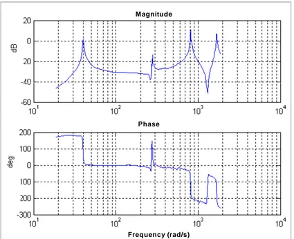
Using a large number of frequencies (between 0 and 2000 rad/s), then by refining our measures around resonance frequencies, we reconstitute an "experimental" Bode diagram representative of the structure motion in steady state harmonic response. We present in Fig. 4 and 5 Bode diagram relative to paths 1-2 and 3-2.
Frequency (rad/s) Phase M agnitude
Fig. 4: Experimental Bode diagram of path 1-2
Frequency (rad/s) M agnitude
Phase
Fig. 5: Experimental Bode diagram of path 3-2
In the interval of frequency between 0 and 2000 rad/s, each path possesses at least 4 resonant peaks (see, Table 2). These peaks are not always the same for each path. However, it is necessary to keep in mind that from a mechanical viewpoint, all modes are present on the structure, but, according to the disposition of ceramics, the contribution of each mode to the measures is more or less negligible.
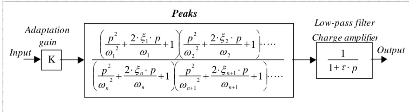
To elaborate a first model, we use the fact that each peak corresponds to a pair of complex conjugated poles. Thus we can represent each peak by a second order system. So, for each path, our model will be constituted by several second order systems and a first order system representing the effect of the charge amplifier. A gain bloc is added. It permits to adapt the static gain of the whole system, as described in Fig. 6. It is an empirical approach.
K p ⋅ + τ 1 1 ⋅ ⋅ ⋅ ⋅ ⋅ ⎟ ⎟ ⎠ ⎞ ⎜ ⎜ ⎝ ⎛ + ⋅ ⋅ + ⎟ ⎟ ⎠ ⎞ ⎜ ⎜ ⎝ ⎛ + ⋅ ⋅ + ⋅ ⋅ ⋅ ⋅ ⋅ ⎟ ⎟ ⎠ ⎞ ⎜ ⎜ ⎝ ⎛ + ⋅ ⋅ + ⎟ ⎟ ⎠ ⎞ ⎜ ⎜ ⎝ ⎛ + ⋅ ⋅ + + + + 1 2 1 2 1 2 1 2 1 1 2 1 2 2 2 2 2 2 2 2 1 1 2 1 2 n n n n n n p p p p p p p p ω ξ ω ω ξ ω ω ξ ω ω ξ ω Input Output Adaptation gain Peaks Low-pass filter Charge amplifier
Fig. 6: Model structure retained for the identification procedure (p is the Laplace symbol)
Making a large number of simulations, we have determined all the parameters (K,ξi,ωi etτ), which allow us to approach at best the actual system.
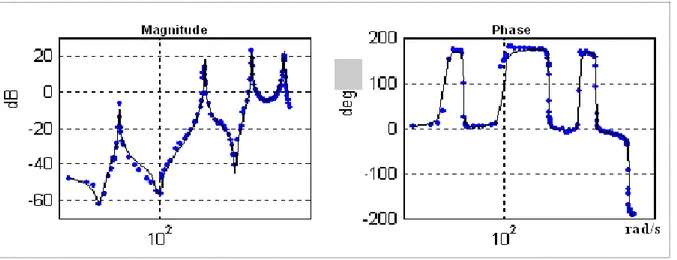
For paths 1-2 results are given in Fig. 7: the curve reflects the model and the cross are experimental points.
Fig. 7: Actual and simulated Bode diagrams for path 1-2
For example, the continuous transfer function corresponding to path 1-2 is given by:
) 10 814 . 2 p 355 . 3 p )( 10 57 . 6 p 863 . 4 p )( 10 854 . 7 p 605 . 5 p )( 1617 p 563 . 0 p )( 1885 p ( ) 10 71 . 1 p 45 . 78 p )( 10 . 967 . 6 p 56 . 10 p )( 05 . 89 p 9437 . 0 p ( 804 59621627.3 G 6 2 5 2 4 2 2 6 2 4 2 2 2 1 + + + + + ⋅ + + ⋅ + + ⋅ ⋅ + + + + + + = −
For paths 3-2, results are given in Fig. 8.
Fig. 8: Actual and simulated Bode diagrams for path 3-2
The two paths present the same resonant frequencies with different magnitudes. But For the anti-resonant frequencies we can notice that they are not exactly the same. The 4 first experimental resonant frequencies of the two paths are given in table 2:
4.2. Finite element model updating and validation
In the active control, the identification is envisaged of different manner according to the mechanic viewpoint or control viewpoint. Indeed, in mechanics the objective of the identification is to obtain geometrical or physical parameters of the finite element model, such as the density mass, the Young modulus or the location of piezoelectric elements stuck on the structure.
Table 2
Resonant experimental frequencies of path 1-2 and 3-2
Mode Frequency (Hz) Frequency (rad/s)
1 6,4 40,21
2 44,1 277,09
4 129 810,53
6 267,4 1680,13
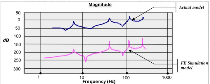
In the framework of our application, if , for example, we compare the Bode diagram of path 3-2 obtained by the FE model to that one obtain by the experimental identification, we observe that differences are essentially due to DC gain (see Fig. 9). This shows the validity of our FE model. What is more, this gain difference is foreseeable in regard to the fact that in the FE model, sensor and actuator amplifiers are not modelized. Hence, by minimizing a criterion characterizing the gap between measures and simulations we perform an updating of the FE model. 300 250 200 150 100 50 0 50 1 10 100 1000 dB Magnitude Actual model Frequency (Hz) FE Simulation model
Fig. 9: Magnitude diagrams of the actual ant the EF model of path 3-2
5. CONTROL AND FDI
In this section, the combined feedback controller and fault estimator design is presented. This integrated approach is based on an algorithm developed by Stoustrup and al. ([15]-[17]). The theoretical framework is briefly described in the following. We recall that in this paper the Laplace variable is denoted p.
5.1. Problem formulation
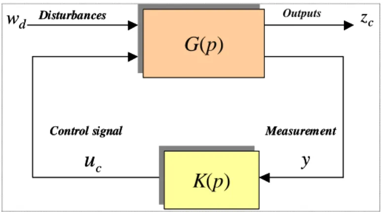
Consider first, a control problem in its standard system configuration as depicted in Fig. 10. Here, is a disturbances or set points signal. The measurements are used by the controller to generate the control signals in order to make the outputs to be controlled sufficiently small (for more details on standard form, please refer to [9]).
d
w y
u zc
G(p)
G(p)
K(p)
K(p)
d w y cu
c z Disturbances Measurement Control signalG(p)
G(p)
K(p)
K(p)
d w y cu
c z Disturbances Measurement Control signal OutputsFig. 10: Standard control problem
This system is described by the following matrix transfer function:
⎟⎟ ⎠ ⎞ ⎜⎜ ⎝ ⎛ ⎟⎟ ⎠ ⎞ ⎜⎜ ⎝ ⎛ = ⎟⎟ ⎠ ⎞ ⎜⎜ ⎝ ⎛ ⎟⎟ ⎠ ⎞ ⎜⎜ ⎝ ⎛ = ⎟⎟ ⎠ ⎞ ⎜⎜ ⎝ ⎛ = ⎟⎟ ⎠ ⎞ ⎜⎜ ⎝ ⎛ c d c d yu yw u z w z c d c u w G G G G u w p G p G p G p G u w p G y z c d c c d c 22 21 12 11 ) ( ) ( ) ( ) ( ) (
The H∞ control problem consists in finding the controller, K(p), that minimize the H∞
norm of the transfer . d
cw
z
G
Suppose now, that the control system is operating under faulty conditions. Hence, one way to model the effect of faults is to consider actuators and sensors faults as additive on the control and the measurement signals respectively. i.e.:
a c s c f and u u f y y = + = +
where fs is sensor fault signal and fa is actuator fault signal.
The goal for the combined approach is to design a single module which in addition to the control signal, also generate a vector signal uf containing estimates of the potential faults:
⎟ ⎟ ⎠ ⎞ ⎜ ⎜ ⎝ ⎛ = s a f f f u ˆ ˆ
Moreover, for a successful individual identification, it is of paramount importance to have good fault models. Hence, we introduce frequency weightings on the fault signals:
a a a s s s W p w and f W p w f = ( ) = ( )
where and are signals that are supposed to have flat power spectra. These are fictitious signals with the sole purpose of generating frequency coloured signals and . For more details on direct faults estimation one can refer to [18] and [19].
s
w wa
s
f fa
The block diagram of the standard control problem is now given in Fig. 11.
G(p)
G(p)
w y u z+
+
Wa(p)Wa(p) Ws(p)Ws(p) a w s w a f s f fu
K
( p
)
cu
c yG(p)
G(p)
w y u z+
+
Wa(p)Wa(p) Ws(p)Ws(p) a w s w a f s f fu
K
( p
)
cu
c yFig. 11: Combined control and fault diagnosis scheme
To transform the system into a new standard H∞ control problem form, we define first the fault estimation error signal:
⎟ ⎟ ⎠ ⎞ ⎜ ⎜ ⎝ ⎛ − ⎟⎟ ⎠ ⎞ ⎜⎜ ⎝ ⎛ = − = s a s a f f f f f f u f z ˆ ˆ
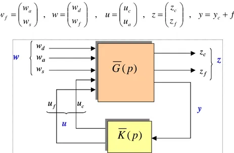
Then we establish a new augmented standard problem (Fig. 12) by defining the following vectors: s c f c a c f d s a f y y f z z z u u u w w w w w w ⎟⎟ = + ⎠ ⎞ ⎜⎜ ⎝ ⎛ = ⎟⎟ ⎠ ⎞ ⎜⎜ ⎝ ⎛ = ⎟⎟ ⎠ ⎞ ⎜⎜ ⎝ ⎛ = ⎟⎟ ⎠ ⎞ ⎜⎜ ⎝ ⎛ = , , , , d w y c u c z a w s w f u
)
( p
K
)
( p
G
zf w z u d w y c u c z a w s w f u)
( p
K
)
( p
G
zf w z uFig. 12: Standard model for the combined approach.
For the new standard problem depicted in Fig. 12, the transfer matrix is given by:
⎟⎟
⎠
⎞
⎜⎜
⎝
⎛
⎟⎟
⎠
⎞
⎜⎜
⎝
⎛
=
⎟⎟
⎠
⎞
⎜⎜
⎝
⎛
=
⎟⎟
⎠
⎞
⎜⎜
⎝
⎛
u
w
G
G
G
G
u
w
p
G
y
z
22 21 12 11)
(
.The explicit formula is:
⎟ ⎟ ⎟ ⎟ ⎟ ⎟ ⎠ ⎞ ⎜ ⎜ ⎜ ⎜ ⎜ ⎜ ⎝ ⎛ ⎟ ⎟ ⎟ ⎟ ⎠ ⎞ ⎜ ⎜ ⎜ ⎜ ⎝ ⎛ − ⎟⎟ ⎠ ⎞ ⎜⎜ ⎝ ⎛ ⎟⎟ ⎠ ⎞ ⎜⎜ ⎝ ⎛ = ⎟ ⎟ ⎟ ⎠ ⎞ ⎜ ⎜ ⎜ ⎝ ⎛ = ⎟⎟ ⎠ ⎞ ⎜⎜ ⎝ ⎛ f c s a d c a s a a f c u u w w w p G s Ws p W p G p G I p W p W p G p W p G p G y z z y z 0 ) ( ) ( ) ( ) ( ) ( 0 ) ( 0 0 ) ( 0 0 ) ( 0 ) ( ) ( ) ( 22 22 21 12 12 11
Introducing the control law: u=K(p)⋅y, the following closed loop system can be obtained:
w p T z= zw( )⋅
where Tzw is given by a Lower Linear Fractional Transformation (LLFT), i.e.:
) ( )) ( ) ( ( ) ( ) ( ) ( )) ( ), ( ( ) ( 1 21 22 12 11 p G p K p I G p K p G p G p K p G F p Tzw = L = + ⋅ ⋅ − ⋅ − ⋅
Hence, the problem is to minimize the H∞ norm of the following transfer: γ
<
∞
zw
T
Stoustrup and al. have demonstrated that, in the certain case, the solution of this problem could be obtained by a kind of separation principle ([15], [16]). Indeed, they pointed out that making the closed loop transfer function associated with the control objectives small and making the closed loop transfer function associated with FDI objectives small can be achieved independently.
For our propose, we have used a state space approach to solve this combined problem ([8]) and [9]). The solution is based on the mix sensibility algorithm.
5.2. Weighted problem
We introduce now control and FDI weights. The H∞ design problem of the combined feedback controller and residual generator is now reformulated in terms of the two-design conditions: Control part: WcTzwWc c d c 2 ∞ <γ 1 FDI part: Wf Tz w Wf f f f 2 <γ 1
where are two weighting matrices relative to control performances and robustness and are two other weighing matrices relative to FDI robustness.
ci
W
fi
W
Without loss of generality, it can be assumed that all weighting functions have been chosen in order to normalize the H∞ standard problem (i.e., 1γc =γf = )
Hence, including weighting matrices in the setup leads to the following transfer matrix:
⎟⎟ ⎠ ⎞ ⎜⎜ ⎝ ⎛ ⎟⎟ ⎟ ⎟ ⎠ ⎞ ⎜⎜ ⎜ ⎜ ⎝ ⎛ − = ⎟⎟ ⎠ ⎞ ⎜⎜ ⎝ ⎛ u w p G W G W G W RW W p G W W G W W G W y z e c e e e c e c c c 0 ) ( ~ 0 0 0 ) ( ~ 22 2 22 2 21 1 2 1 12 1 2 12 1 2 11 1 where:
(
0)
~ 12 12 G Wa G =(
G Wa Ws)
G~22 = 22 ⎟⎟ ⎠ ⎞ ⎜⎜ ⎝ ⎛ = s a W W R 0 0 .This weighing matrix R, influence strongly the FDI problem. Indeed, if R is an identity matrix, the design problem is a fault estimation problem. If R has full rank then it is a fault detection problem.
It is easy to see (as noticed in [15] and [16]) that solving the H∞ design implies making 4 transfer functions/matrices small:
Making
∞
d
cw
z
T small implies good disturbance rejection and robustness. Making
∞
f
cw
z
T small implies that undetected failures do not cause disastrous. Making
∞
d
fw
z
T small will reduce the rate of false alarms. Making
∞
f
fw
z
T small implies good estimation or detection of faults. Hence, to ensure a good control and FDI a careful weight selection is necessary.
6. APPLICATION TO THE COMPOSITE BEAM
The purpose here is to reject the effect of the disturbance on measured signal in presence of possible actuator or sensor faults.
We use the ceramic 1 as actuator and the ceramic 2 as sensors. The piezo-ceramic 3 creates the disturbance. The sampling time is fixed to 6⋅10−4s.
In this paragraph, the experimental results obtained for the controller alone and then for the integrated approach are presented
6.1. Weightings selection
The selection of the weighting functions is a crucial part of the design.
Control part: Here, the focus has only been on disturbances rejection as no tracking references is considered. Hence, the controller has been optimized for rejection of perturbation and FDI specifications. Furthermore, when modeling, we have neglected many modes. Therefore it is necessary to take into accounts omitted modes in order to obtain a robust controller. For that, we have defined multiplicative uncertainty on the output that represent neglected dynamics.
To select dynamic weightings functions, we define the following system:
[
]
⎪⎩ ⎪ ⎨ ⎧ = ⎥ ⎦ ⎤ ⎢ ⎣ ⎡ + ⎥ ⎦ ⎤ ⎢ ⎣ ⎡ = x . C C y u . B B x . A 0 0 A x 0 c 0 c 0 c &where and
{
represent, respectively, the state space representation of the retained and omitted modes. This omitted state part of the system could introduce spill over phenomena while controlling the system.{
Ac,Bc,Cc,0}
Ao,Bo,Co,0}
To avoid this phenomena and to ensure a good disturbance rejection we have selected the two weighting functions ( ) which minimize the classical mixed sensitivity problem (see, [8] and [23] for more details)
2 1, c c W
W
Fault estimation part: As here the goal is to estimate the fault entry, we need to select weighting matrices that permit to scale the fault to the same level. For our application, it was sufficient to scale to fault estimation errors by constant weights. The weight used in design is given by: α = 1 f W
where α is a constant gain depending on the nature of the fault.
Moreover, to ensure a good fault estimation we need either to filter the estimation error or to model the fault signal as the output signal from a low pass dynamic system, i.e.
f W f = f 2
In this application, it is the second method which has been used and the weighting function is selected as “a lawpass” transfer function.
2
f
W
In conclusion, the weighting matrices are adapted to the kind of the fault. is chosen as a constant function, which permits to scale the fault to the same level and as transfert function with first or second order low pass transfer functions.
2 1 and f f W W Wf1 2 f W 6.2. H∞ control results
To elaborate the controller we use the reduced model presented in &4.1. This model is based on the first 3 modes of the identified one (see Fig. 7 and 8). In order to test the robustness of the controller, we apply it to the actual process.
To realize the implantation in real time, each transfer block of the controller is reduced using the classic method based on the comparison of the controllability grammian and the observability grammian ([1], [5]). After reduction of the controller, transfer functions denominators have degrees contained between 8 and 12. During experimentations, we have noted a very good coincidence between simulations and experimentations on the structure.
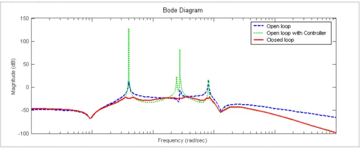
The performance objective is to attenuate vibration due to external disturbances. We present in Fig. 13 the frequency diagram of the open loop and closed loop system of path 1-2. This figure shows a good attenuation of frequency peaks and hence the increase of the damping values of the 3 first modes
Fig. 13: Open and closed loop Frequency response functions of path 1-2
Hence, we present below simulations and actual results for several perturbations and for uncertain system. Parametric uncertainty has been considered (uncertain resonant frequencies,
). % 10 ± r f
Rejection of perturbations with a reduced controller.
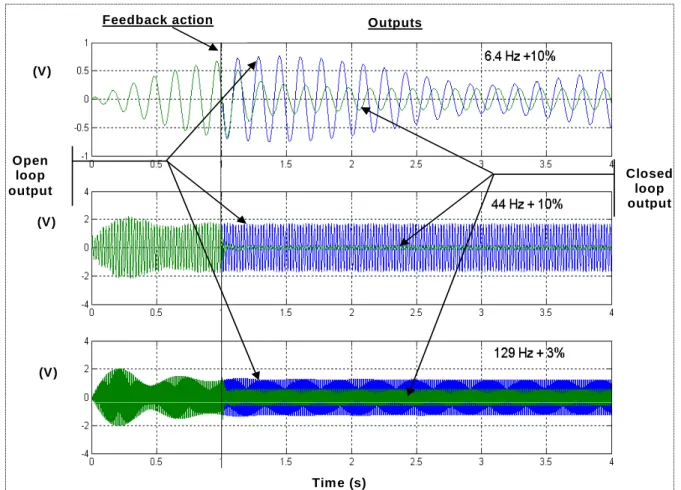
Perturbations are 3 sinusoidal signals exciting the 3 first resonant frequencies of complete model: Feedback action Tim e (s) (V ) (V) (V ) Closed loop output Open loop O utput
O pen and closed loop output
Fig. 14: Simulation for the 3 first resonant frequencies
Fig. 14 presents the time evolution of the system output (Volts) in open loop and in closed loop, when a sinusoidal perturbation is acting on the beam. In the top curve, the perturbation frequency is at 6.5 Hz which is very near of the first resonant frequency. As the figure shows, when the controller is connected (at time t=1s), the output magnitude is reduced in about
. For the middle curve and for the bottom curve, the perturbation frequency is respectively at 44 Hz and 129 Hz (see Table 1). In conclusion, Fig.14 shows that the controller is efficient and rejects the sinusoidal perturbation in an acceptable time. Note that in this approach, the perturbation in not measured.
s 5 . 0 % 10 ± r f
Simulations for model with uncertain resonant frequencies ( ):
Feedback action Outputs
(V) (V) (V) Tim e (s) Closed loop output Open loop output
Fig. 15: Robustness tests: modified 3 first resonant frequencies
The Fig. 15 is analog to Fig.14, but the frequencies of perturbations are modified. The controller has been calculated on the basis of the identified model but the simulations have been performed with a model in which the modal frequencies have been modified. This figure shows the robustness of the H∞ controller. However, it is necessary to insist on ideal conditions of this simulation: the choice of weighting functions is adapted to the frequency of the disturbance and on the quality of the nominal model. Rather than to multiply simulations, it will be more convincing to realize experimentations on the actual structure.
Actual results (using Dspace©) for a sinusoidal perturbation at 6.4Hz:
Fig. 16 shows the output system when a sinusoidal perturbation is applied. In the first part (t<3s), the steady state response is obtained. The controller is connected at time t=3s. This - 19 -
figure shows that the controller is efficient and the rejection is quite good. Note that the actual process is certainly different of the model. Surely, the structure has many eigen modes than those of Table 1, and these modes are not well known. In this experiment, no spillover has detectable.
Closed loop output
Time ( s )
(V) Feedback action
Open loop
Fig. 16: Perturbation rejection for f=6.4 Hz
Actual results for chock type perturbation:
C lo s e d lo o p o u tp u t
T im e (s) (V )
Fig. 17: Rejection of chock type perturbation
For chock type perturbation, the settling time in open loop is about . In Fig. 17, we can notice that with our controller, the perturbations are rejected in about . This shows the efficiency of the closed loop. This comes largely from the choice of the weighting functions that are well adapted to the nature of the disturbance.
s
10
s
3
6.3. Necessity of fault detection
The use of piezoelectric device as sensor or actuator can lead to different kind of failure: • Cracks can appear in the ceramics or in the electrodes,
• Ceramics can be poorly pasted.
• Stressed ceramics due to exposition to a high magnetic field.
If a ceramics is partially detached, the locally physical characteristics of the structure change which implies in addition to faulty measures an alteration of the global behavior of the structure. In the case of occurrence of cracks on ceramics, the global behavior of the structure is not modified but the useful surface of the ceramic is reduced. This kind of faults presents two consequences: a diminution of the gain and a lost of the symmetry of the setting.
Hence, to show the necessity of the FDI procedure, we have performed several simulations. These simulations were carried out in closed loop and by integrating actual measuring noises, which have been measured on the structure. It is a white noise of an estimated variance of 2.58.10-6V2.
We present in Fig. 18 a simulation result for a faulty case. Here, the simulated fault is described as a step function. Fault sensor starts at t=2s and finishes at with amplitude of V. It's a small fault that represents an increase of of the piezoelectric gain. For the closed loop, the controller is connected at t=1 s.
s t=3 3 10 . 5 − 8.3%
C losed loop output
T im e (s) Fault
O pen loop output Feedback action
(V)
Fig. 18: Output with an increase of 8.3% of the sensor gain at 2s≤t≤3s
Fig. 18 shows that we obtain of rejection in 4s when the fault is acting during 1s. This figure indicates that is not possible to detect the fault using only the measure of the output. Of course, as we will see it (Fig. 21), performing detection by analyzing only the output depends on the kind and the magnitude of faults. But, without integrating FDI
% 93
procedure, it is hard to make distinction between fault and perturbation or noise effect. In addition to that, that controller could mask the fault effect on the output because it interprets the fault as a perturbation and would try to reject it.
6.4. Combined module
We apply now the combined design of Fig. 12 to the composite beam. The design was optimized by a judicious choice of weighting matrices in terms of good fault estimation. The weighting matrices have been adapted to the kind of the fault as described before.
2 1 and f
f W
W
We present below some results obtained in the case where the composite structure is corrupted by different kind of sensors and/or actuators faults:
Small sensor fault: We perform here, using the combined design, the same simulation as the
one presented in Fig. 18. This fault represents an increase of of the piezoelectric gain. Here we choose the two weighting functions as
% 3 . 8 0001 . 0 1 , 50 2 1 + = = p W Wf f
The fault estimation signal is depicted below:
Sensor Fault Fault Estim ation
Tim e (s) (V)
Fig. 19: Fault estimation for small sensor fault – increase of 8.3% at 2s≤ t ≤3s
Comments: It turns out from Fig. 19 that integrating now the FDI procedure in the design, allow us to detect the presence of a fault. Indeed, as discussed before, it wasn't possible to decide of the occurrence of a fault by analysing only the output signal. The estimation is quite fast but not very accurate. This is due to the fact that we want to detect small fault in the presence of noise measure.
Important sensor fault: we perform now the same simulation but with a fault signals described as a step function of amplitude of . As it is a big fault its effect on the output is visible on Fig. 20 but the estimation is now quite fast and more accurate.
5 . 0
Fault O pen and closed loop output
Fault Tim e (s) Tim e (s) (V) (V) Feedback action
Fig. 20: Output and fault estimation: Tall sensor fault
• Actuator fault: the fault consists in a modification of the gain actuator. Here the gain is increase as a ramp function entering from t=2s to with a slope of . Fig. 21 shows that fault estimation and perturbation rejection are rather good. s t =4 001 . 0 F a u lt a n d estim a tio n O p e n a n d c lo s e d lo o p o u tp u t T im e (s ) F e e d b a c k a c tio n F a u lt a ctio n T im e (s ) (V ) (V )
Fig. 21: Output and fault estimation: Actuator fault – ramp of slope 0.001 at t=2s
Comments: In Fig. 21, we notice a good tracking of the fault but with a less accuracy. The dynamic of the fault estimation depends on the choice of . It is a trade off between fast and accurate estimation in presence of noises.
2
f
W
The faulty signal is here described as the output of an integrator having a white noise as input. It goes into the system from t =2s to t=4s. This fault simulates a change in the variance of the measured noise.
F au lt s ig n a l O p en an d c lo s ed lo op o u tp ut F au lt actio n F au lt E stim atio n F eed b ack actio n Tim e (s) Tim e (s) (V ) (V )
Fig. 22: Output and fault estimation: noise fault
Comments: Fig. 22 shows the capability of the proposed single module to reject disturbance robustly and to identify which faults have occurred.
7. CONCLUSION
This paper described the design and experimentation of a single module that integrates both robust feedback control action and fault estimation and diagnosis. The experimental set up is a structure made of a composite beam with piezoelectric patches as sensors and actuators.
This work focuses on the necessity of including FDI procedure in any active control strategy to ensure safe applications. The method is based on a formulation of control design and detection design in a scheme of an H∞ optimization problem. We point out the importance of the trade-off between the simplicity of the model and its accuracy in matching the behaviour of the closed loop physical system.
The algorithm proposed is based on H∞ optimization techniques. An important aspect of this method is the trade-off between detection and control systems. Hence, by suitable selection of weights, we can control robustly the system and generate accurate estimation of occurred faults. This permits also to reduce the rate of fault alarms and therefore to increase significantly the reliability of the process. Simulations and experimentations on the actual process have shown the efficiency of the proposed method.
Further work is under way to generate a MIMO fault tolerance control algorithm.
REFERENCES
[1] Gawronski W.K., Dynamics and Control of Structures, a Modal Approach, Springer , 1998.
[2] Chen, J., Patton R.J. Robust Model Based Fault Diagnosis for dynamic Systems. Klumer Academic
Publishers, 2000.
[3] Franck P.M., Ding S.X., Köppen-Seliger B. Current development in the theory of FDI, pp.16-27, 2000. [4] Balas M. J. Active control of flexible structures. Journal of Optimization Theory and Application, Vol.
25, No. 3, pp. 415-436, 1988.
[5] Henriot P., Vergé M. & Coffignal G. Model reduction for active vibration control. SPIE's 7th Annual International Symposium on Smart Structures and Materials, March 2000, Newport Beach, California, USA.
[6] Henriot, P., Mechbal, N., Coffignal, G. & Vergé, M.. Active vibration control and H∞ polynomial fault
detection of a smart flexible structure. Active99, Décembre 1999, Fort Lauderdale, Floride, USA.
[7] Zhou K., Doyle J.C, Glover K. Robust and Optimal control, Prentice Hall, 1996.
[8] Kwakernaak, H. Robust control and H∞ optimization: tutorial paper. Automatica, 29 (2), 1993, pp. 255-273.
[9] Doyle J.C., Glover K., Khargonekar P. & Francis B.A. State-Space Solutions to Standard H2 and H∞
Control Problems. In IEEE Transactions on Automatic Control, Vol. 34, n°8, 1989, pp 831-846
[10] Halim D., Moheimani S.O.R. Spatial Control of Flexible Structures - Application of Spatial H∞ Control to
a Piezoelectric Laminate Beam. In: Proc. ACC, Arlington, June 2001, pp. 4085-4090, 2001.
[11] Qiu Z., Gertler J. Robust FDI Systems and H∞ Optimization. In Proc of the 32nd conf on Decision and
Control, San Antonio, pp. 1710-1715, 1993.
[12] Mechbal, N., Guillard, H. & Vergé, M. An H∞ polynomial fault detection design for uncertain system with time-varying parameters. IFAC SAFEPROCESS 2000, June, Budapest, 2000.
[13] Nett C.N., Jacobson C.A., Miller A.T. An integrated Approach to controls and diagnostics: the 4-Parameter Controller. In Proc of the 1998 ACC, pp. 824-835.
[14] Murad G.A., Postlethwait I., Gu D.W. Robust design approach to integrated controls and diagnostics. In:
Proc. Of the 13th IFAC World Congress, pp199-204, San Francisco, 1996.
[15] Stoustrup J. and Grimble M.J. Integrating control and fault diagnosis: A separation result. Math report No 1996-34, Alborg University, Denmark, 1996.
[16] Stoustrup J. and Niemann H. Application of an H∞ based FDI and Control Scheme for the three-tank system. In Safeprocess 2000, Budapest, Vol. 1, pp. 268-273.
[17] Stoustrup J. and Niemann H. Fault estimation - a standard problem approach. International Journal of Robust and Nonlinear Control, 12:649-673, 2002.
[18] Mechbal, N. & Vergé, M. An approach to optimally robust fault detection. IEEE Conference and Control Application. CCA 20001, September 2001, Mexico.
[19] Niemann H., Saberi A., Stoorvogel A.A., Sannuti P. Optimal fault estimation. 4th IFAC symposium on fault detection supervision and safety for technical process, SAFEPROCESS 2000, Budapest, June, 2000.
[20] Bruant I, Coffignal G, Léné F & Vergé M. A methodology for determination of piezoelectric actuators and sensors geometry on beams structures. Journal of Sound and Vibration, vol 219, (5), 1999.
[21] Mac. A. simple quadrilateral shell element. R. H. Macneal, Computers and Structures, Vol. 8, pp. 175183, 1978.
[22] Ljung L., System Identification – Theory for the user, Prentice-Hall Englewood Cliffs, N. J., 1987.
[23] Kwakernaak, H. Robust control and H∞ optimization: tutorial paper. Automatica, 29 (2), pp. 255-273. 1993.