Stimulation of anticipatory haemodynamics in humans

(1)

(2)

Université de Sherbrooke

Stimulation of Anticipatory Haemodynamics in Humans

By

Gregory Mierzwinski

Radiation Science and Biomedical Imaging Program

Thesis presented to the Faculty of Medicine and Health Sciences in order to obtain a Master’s of Science (M.Sc.) in Radiation Science and Biomedical Imaging.

Sherbrooke, Québec, Canada July, 2020

Members of evaluation committee:

Director: Kevin Whittingstall - Diagnostic Radiology

Internal evaluator: Benoit Paquette - Nuclear Medicine and Radiobiology Evaluator external: Pierre-Michel Bernier – Kinanthropology

(3)

I dedicate this thesis to my parents, Renata Frankiewicz, and Edward Mierzwinski, who supported me throughout the entirety of this endeavour.

(4)

The programmer, like the poet, works only slightly removed from pure thought-stuff. He builds his castles in the air, from air, creating by exertion of the imagination. Few media of creation are so flexible, so easy to polish and rework, so readily capable of realizing grand conceptual structures…

Yet the program construct, unlike the poet’s words, is real in the sense that it moves and works, producing visible outputs separate from the construct itself. It prints results, draws pictures, produces sounds, moves arms. The magic of myth and legend has come true in

our time. One types the correct incantation on a keyboard, and a display screen comes to life, showing things that never were or never could be.

(5)

v

Résumé

Stimulation de l'Hémodynamique Anticipatoire chez l'Homme

Par

Gregory Mierzwinski

Programmes de Sciences des Radiations et Imagerie Biomédicale

Thèse présentée à la Faculté de médecine et des sciences de la santé en vue de l’obtention du diplôme de maitre ès sciences (M.Sc.) en Sciences des Radiations et Imagerie Biomédicale, Faculté de médecine et des sciences de la santé, Université de

Sherbrooke, Sherbrooke, Québec, Canada, J1H 5N4

Le couplage neurovasculaire peut actuellement être mesuré chez l'homme grâce à la combinaison de l'EEG avec des enregistrements BOLD-IRMf. Ces modalités combinées ont considérablement élargi nos connaissances du couplage neurovasculaire, mais ont également montré qu'il existe de nombreux cas où du travail doit être effectué. Il est essentiel de mieux comprendre ces cas marginaux pour comprendre comment interpréter certains résultats. Par exemple, BOLD-IRMf est souvent utilisé pour déduire les changements dans l'activité neuronale des changements dans l'hémodynamique. Mais cette inférence peut décomposer en cas de découplage neurovasculaire. Un tel cas où cela peut se produire est celui de l'hémodynamique anticipatoire qui suggère que le sang peut être pré-alloué aux zones du cerveau en anticipation de l'activation et que la dilatation de la pupille y est corrélée. Cependant, nous n'avons vu ce système que chez des singes macaques et aucune étude n'a encore tenté de reproduire les résultats chez l'homme en utilisant des modalités similaires. De plus, l'étude qui a découvert l'existence de ce système avait une vue très localisée du système et n'a pas entrepris une analyse cérébrale à grande échelle. Cette thèse cherche à répondre à ces préoccupations en effectuant la même expérience sur l'homme et à l'étendre à travers une analyse complète du cerveau pour déterminer les implications qu'elle peut avoir pour notre compréhension du couplage neurovasculaire. Six sujets sains ont été recrutés pour deux expériences: une expérience EEG et suivi oculaire simultanée et une expérience EEG-BOLD simultanée. La réponse EEG de la condition de stimulation anticipative a été comparée à la réponse BOLD mesurée simultanément ainsi qu'aux mesures de suivi oculaire. En effet, il y avait des changements hémodynamiques qui ne pouvaient pas être liés aux enregistrements EEG locaux suggérant que, au moins, le découplage neurovasculaire local se produit lorsque les stimuli sont omis de manière pseudo-aléatoire. Cependant, notre analyse du cerveau complet a révélé des réponses EEG de la région du champ oculaire frontal qui pourraient expliquer les changements hémodynamiques observés dans le cortex visuel par le biais des interactions du réseau cérébral. Ces résultats suggèrent que le découplage neurovasculaire local observé en hémodynamique anticipative peut être contrôlé par une relation de couplage distal.

Mots clés: BOLD, hémodynamique, IRM, EEG, couplage neurovasculaire, suivi oculaire, anticipation, simultané

(6)

vi

Summary

Stimulation of Anticipatory Haemodynamics in Humans

By

Gregory Mierzwinski

Radiation Science and Biomedical Imaging Program

Thesis presented at the Faculty of medicine and health sciences for the obtention of a Master degree diploma (M.Sc.) in Radiation Science and Biomedical Imaging, Faculty of medicine and health sciences, Université de Sherbrooke, Sherbrooke, Québec, Canada,

J1H 5N4

Neurovascular coupling can currently be measured in humans through the combination of EEG with BOLD-fMRI recordings. These combined modalities have greatly expanded our knowledge of neurovascular coupling, but has also shown that there are multiple cases where more work needs to be done. Building a stronger understanding of these edge cases is crucial for understanding how to interpret results. For instance, BOLD-fMRI is often used to infer changes in neural activity from changes in haemodynamics although this inference would breakdown in instances of neurovascular decoupling. One such case where this may occur is with anticipatory haemodynamics which suggest that blood can be pre-allocated to areas of the brain in anticipation of activation and that pupil dilation is correlated to it. However, we have only seen this system within macaque monkeys and no study has yet to try to reproduce the results in humans using similar modalities. Furthermore, the study which discovered the existence of this system had a very localized view of the system and did not undertake a full-scale brain analysis. This thesis seeks to address these concerns by performing the same experiment on humans and expand upon it through a full-brain analysis to determine the implications it may have for our understanding of neurovascular coupling. Six healthy subjects were recruited for two experiments: a simultaneous EEG-Eye Tracking experiment, and a simultaneous EEG-BOLD experiment. The EEG response from the anticipatory stimulation condition was compared to the simultaneously measured BOLD response as well as the eye tracking measurements. We found haemodynamic changes that could not be related to local EEG recordings in the occipital lobe. This suggests that, at the least, local neurovascular decoupling does occur when stimuli are pseudo-randomly omitted. However, our full-brain analysis did uncover EEG responses from the frontal eye field region that could explain the haemodynamic changes observed in the visual cortex through brain network interactions. These results suggest that the observed local neurovascular decoupling in anticipatory haemodynamics may be controlled through a distal coupling relationship.

Keywords: BOLD, hemodynamics, MRI, EEG, neurovascular coupling, eye tracking, anticipation, simultaneous

(7)

vii

Table of Figures

Figure 1. The human brain. ... 1

Figure 2. The anatomy of a neuron. ... 2

Figure 3. The lobes of the brain. ... 4

Figure 4. The occipital lobe subdivisions and the visual pathway. ... 5

Figure 5. Vasculature of the brain. ... 6

Figure 6. Structure of the blood vessels (veins, and arteries). ... 7

Figure 7. The neurovascular unit. ... 10

Figure 8. The canonical haemodynamic response function. ... 17

Figure 9. BOLD signal modulators. ... 18

Figure 10. Sample EEG ICA Components. ... 23

Figure 11. The gradient artifact in a raw EEG time course. ... 26

Figure 12. An example BCG from a single subject average. ... 26

Figure 13. The pupil labs eye tracker. ... 28

Figure 14. Our setup for recording EEG and Eye Tracking simultaneously. ... 30

Figure 15. Visualization of the experiment used in this study. ... 32

Figure 16. Comparison of responses inside vs. outside the scanner... 38

Figure 17. Negative BOLD response in V1. ... 40

Figure 18. Insignificant No-Stim pupillary changes and EEG response. ... 41

(10)

x

List of Abbreviations

3D – Three Dimensional

AFNI – Analysis of Functional NeuroImages BBB – Blood-Brain-Barrier

BCG - Ballistocardiogram

BOLD – Blood Oxygen Level Dependent CI – Continuous Integration

CSF – Cerebrospinal Fluid

CMRO2 – Cerebral Metabolic Rate of Oxygen dHB – Deoxyhemoglobin

EEG – Electroencephalography EPI – Echo Planar Imaging

ERSP – Event Related Spectral Perturbation FEF – Frontal Eye Field

FOV – Field of View

FFT – Fast Fourier Transform

FMRI – Functional Magnetic Resonance Imaging HRF – Haemodynamic Response Function

ICA – Internal Carotid Arteries / Independent Component Analysis IPS – Intraparietal Sulcus

IRM – Imagerie par Résonance Magnétique

IRMf – Imagerie par Résonance Magnétique fonctionnel ISI – Inter-Stimulus Interval

LO – Lateral Occipital LSL – Lab Streaming Layer MR – Magnetic Resonance MCA – Middle Cerebral Artery MRI – Magnetic Resonance Imaging

MNI152 – Montreal Neurologic Institute 152 (subjects) NMR – Nuclear Magnetic Resonance

OBS – Optimal Basis Set

PCA – Posterior Cerebral Artery RF – Radio Frequency

TE – Echo Time TR – Repetition Time

TCP – Transmission Control Protocol XDF – eXtensible Data Format

(11)

Chapter 1: Introduction

A crucial requirement for brain functionality is a constant supply of blood whenever it needs it. This blood is supplied through vasculature, but maintaining a constant supply isn’t as straightforward due to the differences in speed of blood flow versus the speed of neural activity. Human and animal brains accomplish this natural wonder through a phenomenon called neurovascular coupling. But even with this sophisticated mechanism in place, at times, the brain needs to anticipate future blood supply needs in some predictive fashion. This chapter starts with a general overview of the human brain by describing its structure and functional components so that we may build off this knowledge. Then, an explanation of this coupling mechanism, along with how it has been measured will be given. Afterwards, the idea of anticipation, and how it relates to our overall understanding of how the human brain functions will be discussed. Finally, the research conducted in this project, and what knowledge it can provide (or what questions it can answer) will be described.

1.1 The Human Brain

Before going any deeper into various concepts relating to brain functionality, the structure and various components of the brain need to be described. Given that this study is on humans, only the human brain structure will be described. Animals have similar brains though their structure differs greatly and not all animals have a brain whose functionality and composition are similar to a human’s. The human brain is divided into two major components based on

Figure 1. The human brain. We refer to throughs in the folds as

sulci, and peaks as gyri. Reprinted from Parts of the Brain |

Introduction to Psychology, by Lumen Learning, June 24, 2020,

(12)

2 composition: (i) white matter, (ii) grey matter. Grey matter is composed of neurons and glial cells, and white matter is composed of axon bundles that allow distant portions of grey matter (or neurons) to communicate with each other. Grey matter is also organized into folds with each section of the fold having a name. The areas of a fold that are in the shape of a through pointing out of the brain are called gyri while the areas which have throughs pointing towards the inside of the brain are called sulci (see figure 1 (Lumen Learning, n.d.)). However, neither of these components can be fully understood without first understanding the primary functional unit that they contain, neurons.

1.1.1 The Neuron

This basic functional unit of the brain, the neuron, is a cell with many variations and whose functions generally differ depending on where they are in the brain. They are responsible for processing information from our senses to build a representation of the world around us and allow us to interact with it. There are three primary types of neurons in the brain:

motor neurons, sensory neurons, and interneurons. As seen in figure 2 (Hines, 2010), the neuron has a cell body with dendrites and an axon that span outwards from it like arms. Neurons communicate with each other through those arms. The dendrites are used to let

Figure 2. The anatomy of a neuron.The neuron is divided into multiple portions with the axon and

dendrites being the largest portions. The “sending neuron” (presynaptic neuron) passes information to a “receiving neuron” (postsynaptic neuron) through neurotransmitters at a synaptic connection. Reprinted from Chapter 2: Biology and Psychology. The Anatomy of a Neuron by Bernadette Hines, June 24, 2020, retrieved from https://slideplayer.com/slide/5762100/ Copyright 2010 by Cengage Learning.

(13)

3 other neurons send communications to a neuron’s cell body while axons let the neuron send communications by attaching itself to other dendrites. The axon is also coated with a sheath of myelin that helps the cell body’s signal, also called the action potential, propagate towards the axon’s terminals, or synapses. The communications are done through electrochemical signals generated by neurotransmitters at these synapses. The terms pre-synaptic, and post-synaptic refer to axons and dendrites, respectively. Pre-synaptic and post-synaptic potentials refer to where an electrical signal is located. The neurotransmitters responsible for these signals bind to receptors at the post-synapse which cause a change in the membrane potential. When the neuron’s membrane potential (measured in milli-volts) crosses a certain threshold, an action potential (or the electrical signal, which is also referred to as a spike) is produced and this allows it to communicate with other neurons. 1.1.2 Glial Cells

Although neurons are the primary functional unit, cells which support the neurons, called glial cells, are also present in the grey matter of the brain. There are a few varieties, each with their own responsibilities such as providing nutrients for the neurons through astrocytes. The myelin sheath that was mentioned above, which surrounds axons is actually built by a type of glial cell called an oligodendrocyte (Morell P & Quarles RH, 1999). There are many types of glial cells and even though these cells play little role in the actual processing of information they support the neurons which do. One type of glial cell, called an astrocyte, plays a crucial role in the concept of neurovascular coupling by helping bring blood to the neurons when they need it and does so by directly stimulating the local vasculature (Figley & Stroman, 2011).

1.1.3 Functional Divisions of the Brain

Neurons group together to form large circuits and networks that process or pass along some form of information. Local groupings generally deal with one type of information like the visual senses or motor/movement related interactions. That said, areas processing these various pieces of information might be connected through the axon bundles that make up the white matter – some areas do not directly connect to each other. There are 4

(14)

4 major functional areas that are

divided into lobes based on what those sections generally accomplish: (i) the frontal lobe, (ii) the temporal lobe, (iii) the parietal lobe, and (iv) the occipital lobe. (See figure 3 (Wikipedia, 2020) for their locations). Lobes include the white matter and the grey matter in their defined locations whereas the cortex only refers to the grey matter in those areas. Some of the other

areas of the brain, which are not included in these lobes, are the thalamus which acts as a relay system (Sherman & Guillery, 2002), and the brain stem that brings information from the spinal cord to the brain. Recently, the thalamus was found to also be involved in the process of differentiating between types of information and memory (Bolkan et al., 2017; Guo et al., 2017; Schmitt et al., 2017). The frontal lobe is primarily responsible for our cognitive abilities such as learning, and also includes the primary motor cortex for movements (Jawabri & Sharma, 2019). The next one, the temporal lobe, primarily deals with auditory processing. But it’s also an area which integrates the senses such as visual information into memories. Next, the parietal lobe is an area which is involved with integrating senses, generally with visual information, and perception. This area also plays a very large role in spatial reasoning skills, and our sense of touch.

Last but not least, we have the occipital lobe which is the area responsible for visual input processing and the area which this study is focused on. The occipital lobe is quite extensively studied but is still not fully understood. It has multiple functional divisions that can be seen in figure 4 (Joseph, 2018; Trusted Neurodiagnostics Academy, 2020). The

Figure 3. The lobes of the brain. The brain is divided into four main lobes

based on their functions. The divisions are also made through the sulci and gyri. Reprinted from Lobes of the Brain by Wikipedia, June 24, 2020, retrieved from https://en.wikipedia.org/wiki/Lobes_of_the_brain Copyright 2020 by Wikipedia.

(15)

5 sensory input from our eyes is brought to this lobe through the optic radiation tract which originates from lateral geniculate nucleus in the thalamus. Information from each eye is sent to both sides of the brain as shown in figure 4B. The visual information is also flipped upside down in the occipital lobe. All of this visual information arrives at the primary visual cortex called V1. From there, the information is passed up through the visual hierarchy for decision-making. Each division has a particular functionality. For instance, the V5 areas are responsible for image motion processing (Zeki, 2015), while the lateral occipital (LO) areas are thought to be responsible for image or object recognition (Grill-Spector, Kourtzi, & Kanwisher, 2001). But visual information doesn’t only go towards the visual cortex. Since the thalamus is a passage point for sensory input from the eyes, it’s possible that visual information may reach other areas of the brain like the locus coeruleus (located near the pons) through a series of neuronal connections to initiate widespread, or full brain, responses (Samuels & Szabadi, 2008; Weller, Steele, & Kaas, 2002).

Figure 4. The occipital lobe subdivisions and the visual pathway. (A) The subdivisions in the occipital lobe from two views.

The function of the area, if known, is given in parentheses. Reprinted from The Primary Visual Area 17: Occipital Lobe,

Vision, Blind Sight, Hallucinations, Visual Agnosias by Rhawn Joseph, 2000, retrieved from

go from the eyes to the visual cortex. Reprinted from Visual Pathway | Neurodiagnostics EEG by Trusted Neurodiagnostics Academy, 2020, retrieved from https://trustedacademy.com/lessons/veps/visual-pathway-2/

(16)

6 1.1.4 Vasculature

There are two other major components in the brain which are the cerebrospinal fluid, and the vasculature. The cerebrospinal fluid primarily helps with brain maintenance and immunologic protection. But it is also involved with regulating cerebral blood flow (Novak,

Circle of Willis

A

B

C

Figure 5. Vasculature of the brain. (A) Overview of the arteries from the heart to the brain. Adapted from Vascular Supply of the Brain - Clinical Neuroanatomy, 28 ed. by Doctorlib, 2019, retrieved from https://doctorlib.info/anatomy/clinical-neuroanatomy-28/12.html Copyright 2019 by Doctorlib. (B) Sagittal view of the arteries showing a finer detail of where

the PCA artery comes from and goes to. Adapted from Vascular anatomy - NeurologyNeeds by NeurologyNeeds, n.d., retrieved from https://www.neurologyneeds.com/neuroanatomy/brain/vascular-anatomy/ Copyright 2020 by NeurologyNeeds. (C) Overview of the major veins in the brain. Adapted from Blood Supply of the Central Nervous System

(Gross Anatomy of the Brain) Part 2, by The-Crankshaft Publishing n.d., retrieved from http://what-when-how.com/neuroscience/blood-supply-of-the-central-nervous-system-gross-anatomy-of-the-brain-part-2/ Copyright 2020 by The-Crankshaft Publishing.

(17)

7 Krupa, Zlatos, & Nadvornik, 2000) to ensure that there is always just enough blood for neurons since they are sensitive to heightened and suppressed levels of blood flow (or over- and under- perfusion) (Cipolla, 2009). This blood flow comes from the vasculature of the brain with arteries supplying blood to the brain, and veins draining deoxygenated blood (or deoxyhemoglobin) from the brain. Figure 5 (Doctorlib, 2019; NeurologyNeeds, n.d.; The-Crankshaft Publishing, n.d.) shows an overview of both of these structures and where they are placed. Note that both of these vascular portions are structured as tube-like branches, with an increasingly small basal diameter as we move away from the main branches. The main arterial branches begin with the internal carotid arteries (ICA) that flow to the Circle of Willis, and then branch into the three primary branches supplying blood for the brain: (i) the middle cerebral artery (MCA), (ii) the anterior cerebral artery (ACA), and the posterior cerebral artery (PCA). The PCA is responsible for bringing blood to the occipital lobe in the posterior section of the brain. At the other end of the blood cycle we find the veins which connect to the arteries in a structure called the capillary which is where neurons receive blood (oxyhemoglobin) and return used blood (deoxyhemoglobin). Veins, which are also named sinuses, drain deoxyhemoglobin from the brain. Although there are a multitude of

Figure 6. Structure of the blood vessels (veins, and arteries). Note how the size of the

artery is larger than the veins due to the differences in blood pressure that they must sustain. Reprinted from Blood vessel - Wikipedia by Kevinsong, 2013, retrieved from

(18)

8 cerebral veins, the ones that are most related to this project, and are located in the posterior of the brain are: (i) the superior sagittal sinus, (ii) the occipital sinus, and (iii) the confluence of sinuses. All cerebral veins eventually make it to the jugular vein which returns the deoxyhemoglobin to the heart. The structure of these blood vessels is shown in figure 6. Inside the blood vessels we find the nutrients which flow around the body such as oxygen and glucose. The walls are layered and in the inner layer we find the endothelium cells which are responsible for changing the diameter of the blood vessel. On the outside of the blood vessel we find pericytes which are responsible for communicating with the endothelium cells to initiate the changes in diameter. There is also a layer of smooth muscle around the vessels that constricts and dilates the blood vessels. Both veins and arteries have these mechanisms for constriction and dilation but the walls of the veins (and therefore its components) are thinner since the blood pressure in veins in lower (OpenStax, 2016). As we move from the circle of Willis, the arteries become pial arteries that traverse the outside of the cortex. When they begin penetrating the brain, they become arterioles, and finally capillaries. Each portion has a different structure, with the smooth muscle layer becoming thinner as we move towards the capillaries. In the brain, there is a strong barrier between brain matter and its blood supply, aptly named the blood-brain-barrier (BBB). This is here to protect the brain from toxic material in the blood and to tightly regulate what can flow into the brain. This barrier is formed by the cells which line the capillary, along with the endothelial cells lining the inside of blood vessels (since capillaries are where neurons, and other cells obtain their nutrients) (Daneman & Prat, 2015). All blood vessels also have what is called a basal tone, which is the diameter (or level of contraction/dilation) of the blood vessel at rest. Cerebral blood flow, also named perfusion, is regulated by differences in pressure, or pressure gradients. For the sake of generality, we can assume that we have a steady laminar flow (though this is not always true as blood fluid behaves in a non-Newtonian way), allowing us to model it by the following equation named Poiseuille’s Law (Fantini, Sassaroli, Tgavalekos, & Kornbluth, 2016):

𝐵𝑙𝑜𝑜𝑑 𝐹𝑙𝑜𝑤 = ∆𝑃𝜋𝑟 4

(19)

9 It is based on Ohm’s Law which states that a flow is proportional to the pressure gradient, and the resistance of a material to that flow, or that 𝐹𝑙𝑜𝑤 = 𝑃𝑟𝑒𝑠𝑠𝑢𝑟𝑒 𝐺𝑟𝑎𝑑𝑖𝑒𝑛𝑡 / 𝑅𝑒𝑠𝑖𝑠𝑡𝑎𝑛𝑐𝑒. Poiseuielle’s Law is modified for blood flow where 𝐿 is the length of the blood vessel, 𝑛 is the viscosity of the blood, and 𝑟 is the radius of the blood vessel. As shown in the equation, the radius of the blood vessel is by far the largest factor in determining the blood flow meaning that small changes in radius can lead to large impacts in blood flow. In the PCA, as we move closer towards the cortex of the occipital lobe, we find smaller radii for blood vessels. But those vessels also have the largest change in blood flow when they become active because they have the largest percent-based change in radius (Bizeau et al., 2018). In larger vessels, their change in vessel diameter is smaller so they have a smaller change in blood flow. This vasodilation phenomenon is actually propagated along the arterial branches. However, it is still unknown whether these stimulus-induced changes are caused by something at the receiving end or something closer to the point of origin of the blood flow.

1.1.5 Summary

Putting this all together, the human brain is a highly complex organ and these descriptions of the various sections only scratch the surface of it. Although there are 4 major functional lobes, studies of each of those lobes have been significantly expanded upon and can be broken down into even smaller functional areas, like how the occipital lobe is divided into a visual hierarchy. The vasculature, glial cells, and cerebrospinal fluid which support these functionalities are crucial for the brain’s survival since this organ can consume up to 20% of the body’s energy supply. How exactly these various components work together to keep the neurons nutrient supply at a reasonable level without killing the cells required for proper functioning is the subject of the next section on neurovascular coupling.

1.2 Neurovascular Coupling

All nutrients that a neuron requires to survive and perform its functions are supplied through the vasculature. But keeping a steady supply to all parts of the brain simultaneously

(20)

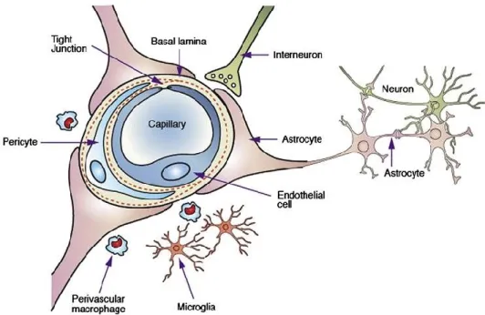
10 is a feat of its own. Having too much flowing in can result in abnormally high levels of pressure that could damage the soft tissue of the brain. While having too low can lead to neuronal death because of a lack of resources. Neurovascular coupling is the concept by which this interplay of resources and activity is regulated. This coupling starts with the basic neurovascular unit which is shown in figure 7 (Salunkhe, Bhatia, Kawade, & Bhatia, 2015). The astrocyte is a glial cell which draws nutrients from the blood vessels (capillaries or arterioles in this case) to the neurons and also releases chemicals which cause vasodilation or vasoconstriction. The blood vessel responds to those chemicals by either contracting or dilating. There are also other portions of this unit, that may include neurons, that release a chemical to cause vasodilation either directly or indirectly through glial cells. The debate is still ongoing for how exactly this mechanism works as there are many possibilities for how vasculature can be innervated (Hosford & Gourine, 2019). Some experiments have also shown that nitric oxide (NO), released by an astrocyte’s end feet, can innervate arteries to cause dilations (Muñoz, Puebla, & Figueroa, 2015). In animals, we can measure this coupling mechanism invasively and non-invasively. Optical imaging of an animal’s cortex can be combined with electrodes to simultaneously measure changes in arterial

Figure 7. The neurovascular unit. Neurons primarily receive their nutrients from astrocytes, and

some neurons also directly innervate the blood vessels (interneurons). Reprinted from

(21)

11 oxyhemoglobin concentrations and neural activity, respectively. In humans, we can’t easily do these kinds of in-vivo tests on large groups of subjects. Instead, we use non-invasive techniques such as simultaneous electroencephalography (EEG), and blood-oxygen-level-dependent (BOLD) functional magnetic resonance imaging (fMRI). EEG measures large-scale changes in neural activity (measuring large pools of neurons rather than individual ones) that are detected through changes in scalp potentials. BOLD-fMRI measures changes in the levels of deoxyhemoglobin which are usually tied to changes in the cerebral metabolic rate of oxygen (CMRO2) and blood flow caused by neuronal activity. In other words, changes in BOLD-fMRI are thought to be related to neural activity through neurovascular coupling and we can check if this relation is true by combining these tools. Unfortunately, this pairing doesn’t work for looking at changes deep within the brain in areas like the thalamus due to the limited spatial resolution of EEG, though some have recently claimed that this is possible with measurements taken with high-density EEG (Seeber et al., 2019). See Chapter 2 for more information on these tools, as well as how they are combined.

1.3 Neurovascular Decoupling

Neurovascular coupling is believed to always occur; for any change in cerebral haemodynamics, there’s an associated change in neural activity. However, in recent years, this association has been questioned and researchers have been reporting cases of neurovascular decoupling, or dissociation of neural activity from haemodynamics. In humans, researchers found that pathologies could be responsible for producing neurovascular decoupling (Para et al., 2017; Peca et al., 2013; Yu et al., 2019), but none have shown this can occur in healthy subjects. In mice, it’s been shown that astrocytes could cause changes in haemodynamics without any change in neural activity (Takata et al., 2018). Then in monkeys, two researchers found, what they call, anticipatory haemodynamics might be capable of inducing decoupling.

(22)

12 1.3.1 Anticipatory Haemodynamics

Anticipatory haemodynamics were first observed by the researchers Das, & Sirotin in a study published in 2009 (Sirotin & Das, 2009). There, they trained monkeys to observe a visual stimulus but during experimentation, they pseudo-randomly omitted a stimulus. When this omission occurred, they noticed that there was a lack of neural activity observed in the primary visual cortex (or V1), but found that the haemodynamic response was still observable in this area in the form of a dilation of the blood vessels occurring in anticipation of the stimulus arrival. Furthermore, when an auditory task was used, they noticed that the haemodynamic response was no longer visible in the visual cortex, suggesting that this anticipatory response was stimulus-specific, and that it was not a whole-brain phenomenon. The researchers used an electrode implanted in the brain to measure neural activity, and an invasive optical imaging technique to measure the haemodynamic response. They concluded that the anticipatory response was not predicted by local neuronal activity and that it was correlated with pupillary dilations. This also marks the first time that these anticipatory haemodynamics were observed. However, this statement was met with a high degree of criticism (Das & Sirotin, 2011; Friston, 2012; Handwerker & Bandettini, 2011b, 2011a; Kleinschmidt & Müller, 2010) since it went against the concept of neurovascular coupling and seemed to show neurovascular decoupling. However, these are not unwarranted as there are some major faults in their methodology such as using a single electrode for measuring neural activity. Though to be fair, the researchers did stress that their results only support the idea of localized neurovascular decoupling, and does not rule out that the changes could be neuronally initiated through distal neurovascular coupling, or by a small group of immeasurable neurons. Regardless of this criticism, the question remains, if neurovascular coupling holds true why is there no local measurable neural activity when changes in haemodynamics are observed? Multiple possibilities exist for why this occurs such as (i) distal neuromodulatory mechanisms, or (ii) very small groups of immeasurable neurons controlling the haemodynamic response (Cardoso, Lima, Sirotin, & Das, 2019). But these are hypotheses and have not yet been proven, leaving the possibility open for neurovascular decoupling to exist in situations like this where it seems

(23)

13 that blood is delivered to areas of the brain in anticipation of an upcoming task without requiring action from neurons. Enhancing our understanding of this coupling mechanism is crucial to be able to properly build new measurement tools for neuronal activity. Our understanding of what our current tools are measuring also relies on this understanding. Should it break down under certain circumstances, experimental results could be misinterpreted. This would continue to be true even if coupling is shown to always be true on a very small scale, but breaks down in less invasive measurements. Shedding light on exactly what is being measured in these experiments may also provide interesting avenues of future research for anticipatory drug delivery mechanisms, or new methods of measuring pathologies.

1.4 Proposed Approach

Given the importance of understanding how neurovascular decoupling works, the primary purpose of this project is to replicate the findings of Das, & Sirotin in humans. To our knowledge, there are no studies which have done this. One study has shown that a haemodynamic response is observable in the visual cortex when a visual stimulus is pseudo-randomly omitted when performing similar experiments (Ress, Backus, & Heeger, 2000). They also found that these responses are almost identical, in both size and shape, to those produced by a visual stimulus. When conducting visual tasks in humans, it is widely understood that neurovascular coupling can be measured by correlating high-frequency changes in neural activity (named gamma-band power) measured with electroencephalography (EEG) with the haemodynamic changes observed in Blood Oxygen Level Dependent Functional Magnetic Resonance Imaging (BOLD-FMRI) measurements (Ebisch, Schmidt, Niessing, Singer, & Galuske, 2005; Koch, Werner, Steinbrink, Fries, & Obrig, 2009; Logothetis, 2003; Logothetis, Pauls, Augath, Trinath, & Oeltermann, 2001). But this relationship has been shown to break down because the gamma-band responses are no longer measurable but changes in haemodynamics still occur (Drew, 2019; Swettenham, Muthukumaraswamy, & Singh, 2013). These suggest that measuring neurovascular

(24)

14 coupling can break down in certain situations, making it plausible for the anticipatory response to be another form of neurovascular decoupling that is measurable in humans. 1.4.1 Objective

Although some studies have performed similar stimulus-omission experiments with agreeing results (Ress et al., 2000; Takata et al., 2018), there are no studies that have simultaneously measured neural activity alongside haemodynamic responses and conducted a full-brain analysis of the measurements in humans. This work aims to fill that gap of knowledge. We hypothesize that when we measure neural activity and haemodynamics simultaneously with this experiment, we will find neurovascular decoupling. We will attempt to replicate these findings using EEG and BOLD-fMRI. Furthermore, since it’s been shown that pupil diameter correlates with these anticipatory haemodynamics we will also perform a simultaneous EEG and eye tracking experiment. This experiment will provide us with EEG data that are not contaminated with MRI-induced artifacts to validate our in-scanner recordings, and allow us to validate the observed pupil dilations observed in macaque monkeys.

These two experiments will let us obtain a full brain picture of what is happening during these random stimulus omissions. With this we will be able to greatly expand on what the researchers had originally found. To complete this objective, we first had to implement a method to measure data from our EEG and eye-tracker simultaneously. We completed this, and a description of the work involved can be found in the Eye Tracker section in Chapter 2. With that, we recruited 6 subjects that went through two experiments. These were very similar to the original experiment in that there was a visual stimulus omitted randomly and more on this experiment can be found in the next chapter. Finally, after obtaining the data, we had to analyze it to determine if there are any changes in haemodynamics that cannot be correlated to observable changes in neural activity. What we found through this effort is described in chapter 3.

(25)

15

Chapter 2: Material & Methods

This project employs multiple measurement modalities: Magnetic Resonance Imaging (MRI), Electroencephalography (EEG), and Eye Tracking. Functional MRI is used to measure the haemodynamic changes, while EEG will be used to measure the observable neural activity from the scalp. Eye tracking is also used to detect changes in pupil diameter since it has been shown that dilation of the pupil correlates with changes in haemodynamics when performing anticipatory experiments. The following sections of this chapter will first present an introduction to the aforementioned measurement techniques as well as how data recorded from these modalities is processed. For eye-tracking, the work produced through this project, as a prerequisite to the experiments, will also be described. This will be followed by a description of the experiments that were performed on the human subjects.

2.1 Magnetic Resonance Imaging

Measuring changes in vasculature of the human brain has to be done non-invasively to be able to gather data from the widest possible range of subjects. One of the techniques we use to do this with is Magnetic Resonance Imaging (MRI), which allows us to produce 3-dimensional images of the entire brain. This modality works by taking advantage of a phenomenon known as nuclear magnetic resonance (NMR). NMR comes into play when an atom is excited by a radio-frequency (RF) pulse inside a magnetic field. When the atom begins to return to its stable state, it emits a radio-frequency signal that can be measured, in other words, this emission releases the energy that was gained through the initial RF pulse. While any atom can be stimulated in this way, in MRI, the hydrogen atom is targeted because it is the most abundant in the body (in water) and therefore provides the strongest signal we can use. In MRI, this signal can be modified by the surrounding environment which can change its rate of decay and these differences in decay rates give rise to the contrast we see in our images.

(26)

16 To understand the following sections, we need to know a bit more about how MRI works. It all starts with the magnetic field that the MRI produces - often called the 𝐵0 magnetic field. This aligns the majority of the spins, or magnetic moments, of the hydrogen atoms to point in the same direction as 𝐵₀. In other words, the average net magnetization of these spins is in the direction of 𝐵₀ and many spins might not be aligned to it. Furthermore, they aren’t perfectly aligned and they rotate around the net magnetization direction (precession); moving around it at a rate that is called the Larmor frequency that depends on the strength of 𝐵₀ and the gyromagnetic ratio (specific to each element or particle). To give energy to these atoms, the RF field that the MRI briefly emits needs to produce a magnetic field, often called 𝐵1, that is rotating at the Larmor frequency. An analogy that is often used here is the idea of pushing a child on a swing – there’s a particular resonant frequency of pushing that returns a maximized response. The hydrogen atoms absorb this energy and it pushes the tip of the net magnetization 90° away from 𝐵0 (into the transverse plane). At this stage, the tip of the net magnetization is precessing perpendicularly from the direction of 𝐵0. By Faraday’s Law of Induction, a current can be generated in a coil using this rotating net magnetization and this is essentially what we measure with an MRI machine.

The precession in the transverse plane decays due to its environment and the spins return to the most stable energy state. This decay occurs because the phase coherence of the spins in the transverse plane begin to decrease. But one of the ways to keep the precession going for longer is by applying a 180° RF pulse that reverses the spin dephasing and allows us to produce an echo of the original signal. The time at which the 𝐵1 RF pulse is repeated during imaging is called the repetition time (TR) and the time between this pulse and the center of the echo is called the echo time (TE). By modifying these values, we can produce images with varying contrasts depending on the relaxation rates (decay rates) of this precession in tissues that are being targeted. There are two types of relaxation rates: (i) T1 relaxation which is the rate at which the net magnetization in the direction of 𝐵0 returns to its maximal amplitude, and (ii) T2 relaxation which is the rate at which the transverse magnetization returns to 0. Using short TR and TE settings produces images which are T1-weighted and

(27)

17 using long TR and TE settings produces images that are T2-weighted. In a T2-weighted image, we will find that the cerebrospinal fluid (CSF) is bright, whereas T1-weighted images have dark areas where the CSF should be - CSF has a lot of water with less inhomogeneities that could dephase the signal.

2.1.1 Blood-Oxygen-Level-Dependent Contrast Imaging

There are two types of images that can be generated using MRI: (i) static, and (ii) dynamic. The static images provide a single 3-dimensional volume that is a snapshot of what we see. These are produced for standard anatomical images. Dynamic imaging sequences on the other hand produce 4-dimensional volumes, where we obtain multiple 3-dimensional images over time. This is also called functional MRI (fMRI) because we are usually measuring functional activities within the brain that occur during an MRI scan. One of the most widely used is called Blood-Oxygen-Level-Dependent (BOLD) fMRI. This technique measures T2* relaxation rates which include the T2 relaxation rate, but are also affected by magnetic field inhomogeneities caused by things like the presence deoxyhemoglobin (dHB) which is paramagnetic due to its four unpaired electrons. With this type of sequence, we can actually measure changes in the concentration levels of deoxyhemoglobin in the brain. When concentrations of dHB increase, this leads to a faster dephasing which leads to a lower signal, and when concentrations decrease the opposite occurs.

Figure 8. The canonical haemodynamic response function.

Reprinted from BOLD and Brain Activity - Questions and

Answers in MRI by Allen D. Elster, 2020, retrieved from

http://mriquestions.com/does-boldbrain-activity.html

(28)

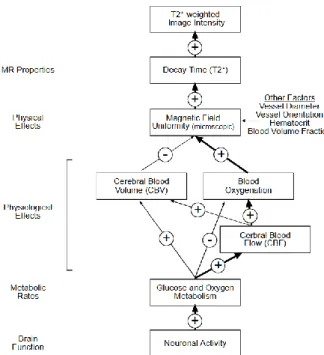
18 BOLD is believed to measure neural activity indirectly and this has been shown to be true in multiple cases. Anytime a human is stimulated in some way, the areas of the brain which activate can be found by looking for a theoretical haemodynamic response shown in figure 8 (Elster, 2020). This response function starts with an initial dip, which has never been seen in actual experiments because the temporal resolution of BOLD is quite poor, but it is believed to be caused by a decrease in the concentration of oxyhemoglobin caused by neural activity. This neural activity initiates a vascular reaction that brings in oxygenated blood that decreases deoxyhemoglobin concentrations and increases the BOLD signal which causes the large peak we see. Finally, the signal returns to its baseline value and proceeds even further down to what is called the BOLD undershoot. This undershoot exists and is measurable but what actually causes it is still a matter of debate. Note the time scale in figure 8 as well, the BOLD peak doesn’t occur until at least 5-7 seconds after a stimulation begins. That said, we can’t be completely positive about what causes changes in BOLD images because there are too many factors that can cause it to change (figure 9 (Noll, 2001)). But it doesn’t diminish the potential of BOLD to be, at the least, a simple and easy to use technique (and cheap relative to other methods). Most changes in vasculature will be picked up by BOLD in some way, and this allows us to use BOLD as a starting point to determine if there is more that needs to be looked at with tools that probe more specific vascular changes.

Figure 9. BOLD signal modulators. Plus signs refer to positive

correlations, whereas negative signs refer to negative correlations between the linked modulators. Reprinted from A primer on MRI

(29)

19 2.1.2 Pre-processing

In this project, we used a very fast BOLD imaging sequence on a 3T Philips Ingenia with the following parameters: a TR/TE of 672/30 ms, a flip angle of 50°, field-of-view (FOV) of 240 X 240 X 123.75 mm, voxel size of 3 mm (isotropic), a multiband (MB-SENSE) acceleration factor of 6 (only slice acceleration (MB-SENSE = 6) was used, without in-plane acceleration (SENSE = 1)). An anatomical T1-weighted 3D gradient-echo image (a TR/TE of 7.9/3.5 ms, a flip angle of 8°, a FOV of 240 X 240 X 150mm, and a voxel size of 1 mm (isotropic)) was acquired after the FMRI acquisitions. All of these acquisitions were performed with a 32-channel head coil. When we obtain BOLD images from the experiments that we perform, there are a few things that need to be fixed before the data can be analyzed. The first correction that needs to be made is for motion. While the subjects are positioned in a manner that makes it difficult for them to move (because of the head coil), it doesn’t stop them from drifting slightly over time. Even though this movement is quite small it has a huge impact on our measurements because of the small size of our voxels. We correct for this using a tool called mcflirt (Jenkinson, Bannister, Brady, & Smith, 2002). It takes a template image, in our case it was the middle volume in the BOLD time series, and performs image registration to move all the other images in the time series to be as closely aligned as possible to it. Image registrations use various cost functions to define the correctness of the registration and guide algorithms in the direction of the best possible registration. There are two types of registrations: (i) linear which apply the same transformation on all portions of the volume equally, and (ii) non-linear which apply different transformations on different portions of the volume. Both of these will scale, rotate, translate, or shear the images to find the best possible fit according to the cost function.

After we complete motion correction there is still one more artifact left to remove. This artifact shows up as a slow drift in the time series data and it’s primarily caused by physiological effects like breathing. Generally, we can remove all signals which have a frequency of less than 0.1 Hz as they are unlikely to be related to the functional activity that is being performed. We use a high-pass filter through a tool called 3dBandpass (a part of AFNI) to remove these (Cox, 1996). We could also perform a band-pass filter here to remove

(30)

20 the high frequency noise if needed. Once this is complete, the data is ready to be analyzed. The analysis is generally performed by searching for areas in the brain that reacted to a stimulation by comparing the signal in various regions to the HRF mentioned above. There are also other techniques that can be used such as the Student’s T-test or Z-score to find areas which had a sufficiently large change, regardless of the full shape of the change. In this study, we correlated the HRF with the BOLD signal to find regions of activation, this is discussed further in section 2.6.4.

2.2 Electroencephalography

To measure changes in neural activity non-invasively in humans, we use electroencephalography (EEG). It uses a cap, similar to a bathing cap, that is placed on a person’s head with multiple electrodes inserted into it and positioned according to standardized orientations i.e. the 10-20 system. These electrodes are used to measure changes in the electric potential on the scalp that are caused by changes in neural activity. As mentioned earlier, with EEG we measure large pools of neurons rather than small groupings, or individual ones so we can’t say that changes in neural activity are caused by an increase or decrease in the number of active neurons. We can only say that the neural synchrony changes with this modality and synchrony generally refers to the degree of in-phase activations within some population of neurons (Timofeev, Bazhenov, Seigneur, & Sejnowski, 2013). This synchrony can be long-range or short-range and can occur through a few different routes (e.g. chemical synaptic mechanisms, ephaptic interactions, changes to extracellular ionic concentrations). That said, changes in the number of active neurons can influence EEG measurements as well so the term synchrony is inherently ambiguous. EEG measurements originate from under the scalp and are thought to be primarily driven by pre and post synaptic potentials more than action potentials (Nunez & Srinivasan, 2006). The primary reason for this is that action potentials evoke very high-frequency responses which are largely attenuated over large distances. Pre/post synaptic potentials are responsible for what is called the local field potential whose oscillations have lower

(31)

21 frequencies, and have been shown to be strongly coupled to changes in scalp measurements (Creutzfeldt, Watanabe, & Lux, 1966; Klee, Offenloch, & Tigges, 1965). When multiple neurons activate in-phase (synchronized) with each other, these local field potentials become amplified and interact constructively, making them measurable from the scalp. In contrast, when neurons are desynchronized with each other, the local field potentials interact with each other destructively to attenuate the measurements we obtain on the scalp.

2.2.1 Neural Oscillations and Rhythms

After recording data from EEG, we obtain 64 time series, or one for each electrode that was recorded (64 electrodes is the standard amount). The data are measured in millivolts and can be recorded at various sampling rates. Generally, a 500Hz sampling rate is more than enough to capture all neural oscillations that are measurable from the scalp which go up to approximately 120Hz. These neural oscillations have been divided into several groups depending on their frequency of oscillation.

The lowest frequency band is called the delta rhythm which ranges from 0.5-4Hz and is usually related to sleep. The next band is called theta and ranges from 4-7Hz. After this, we find the alpha band rhythm which ranges from 8-13Hz. This band of frequencies has also been called the Berger rhythm and becomes very prominent when subjects close their eyes. From 13-30Hz, we find the beta rhythm that has been shown to be related to various sensory processing phenomena, most notably, in movement related activities (Baker, 2007). Everything else, from 30Hz+ or from 30-120Hz, forms what is called the gamma band rhythm. This band of frequencies has been related to feedforward activity, or activity that is related to sensory input such as changes in information moving from the eyes to the visual cortex (Bastos et al., 2015). In contrast, the alpha-band has been related to feedback-related neural activity, or activity that occurs after a sensory input has been processed and information is returned towards the point of origin of the sensory input. Some of these bands, such as gamma, have also been sub-divided into low, high variants in recent years (Griffiths et al., 2019; Kucewicz et al., 2017; Solomon et al., 2017) as well as narrow and broadband responses (Bartoli et al., 2019). The haemodynamic measurements obtained

(32)

22 from BOLD fMRI are currently believed to index both the feedforward (gamma) and feedback (alpha) activity with variable contributions from each of them (Butler, Mierzwinski, et al., 2019).

When the EEG data are analyzed based on these bands of frequencies, increases and decreases in the power of those rhythms is referred to as synchronization, and desynchronization, respectively. That said, this concept is specific to EEG measurements of neural activity. When intra-cranial measurements that are more localized are used, changes in synchronization can refer to changes in how much different areas of the brain are synchronized or work together. For measurements that use a single electrode, power refers to the same thing it refers to in EEG but for a smaller region. This is an important distinction that needs to be made when comparing studies using EEG to studies using invasive neural recordings as the nomenclature used in these studies is ambiguous.

2.2.2 Pre-processing

In this project, for the experiments that were performed outside the scanner, we used the 64-electrode EEG cap (ActiCap) from BrainVision following the 10-20 system for electrode positioning. During the experiments, it was recording at a sampling rate of 500Hz. Pre-processing the data simply involves cleaning out the noise from the data. First, the data might be resampled to a different sampling rate than what was recorded. Based on the Nyquist theorem, if frequencies up to 120Hz need to be observed, a sampling rate of at least 256Hz would be required so this is the minimum that the data should be resampled to if all responsive frequencies are to be analyzed. After this, some cases will require notch filters to remove electrical line noise from the data at 60Hz and 85Hz (leaving all the other frequencies unchanged). Once the sampling rate is properly set, and all noisy frequencies are removed the data can be analyzed. However, there are still some other sources of noise that have a physiological origin such as eye blinks which might need to be removed since they can interfere with the stimulus recordings. To do this, we employ a technique called Independent Component Analysis (ICA) that allows us to separate the various linearly-combined sources of neural activity in electrode recordings into single components (up to 64 components with a 64-electrode EEG cap).

(33)

23 Implementations of this technique work by starting with an N-X-dimensional matrix, in our case a 64-X-dimensional matrix, where X is the length of the time series recorded. Some preprocessing may be performed on the data to remove any correlations from it, this is often called whitening or sphering the data. Then, this matrix is essentially rotated to minimize the amount of mutual information between the electrodes. Defining mutual information is where the implementations usually differ. Some algorithms maximize non-gaussianity of the data while others might minimize mutual information when they choose rotations (Erdogmus, Hild, Rao, & Príncipe, 2004). This mutual information is generally calculated between the projections of the data at each of the 64 axes of the matrix. These calculations produce a C-64-dimensional weighting matrix (a rotation matrix, also called a mixing matrix) where C is the number of components. This can be multiplied with the data matrix to produce a 64-X-dimensional matrix where each row is a component:

𝐼𝐶𝐴 𝐶𝑜𝑚𝑝𝑜𝑛𝑒𝑛𝑡𝑠 = 𝑊𝑒𝑖𝑔ℎ𝑡𝑖𝑛𝑔𝑠 ∗ 𝑂𝑟𝑖𝑔𝑖𝑛𝑎𝑙 𝐷𝑎𝑡𝑎

Each column of this weight matrix provides weightings that are applied to each electrode’s time series to produce a component, i.e. each component has one weighting per electrode so it does not vary temporally. Furthermore, each component is a combination of changes from all electrodes so these components are not in source, or electrode, space.

Given that the mutual information between the electrodes was minimized, this product produces components whose statistical independence from one another was maximized. Artifacts like eye blinks occur independently of the stimulus related changes and do not

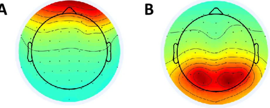
A

B

Figure 10. Sample EEG ICA Components. A) An ICA component caused by blinks. B) An ICA

(34)

24 vary temporally so they can be easily separated as a statistically independent component using ICA. For instance, in figure 10A, we see a topographical view of an inversed EEG weighting matrix column for a blink component (anterior activation), and in figure 10B, we see a component that is related to a visual stimulation (posterior activation). Once we find the visual components they can be averaged together, or processed individually. These could also be projected back into the source space by using the inverse of the weighting matrix:

𝐸𝑙𝑒𝑐𝑡𝑟𝑜𝑑𝑒 𝑆𝑝𝑎𝑐𝑒 𝐶𝑜𝑚𝑝𝑜𝑛𝑒𝑛𝑡𝑠 = 𝐼𝑛𝑣. 𝑊𝑒𝑖𝑔ℎ𝑡𝑖𝑛𝑔𝑠 ∗ 𝐼𝐶𝐴 𝐶𝑜𝑚𝑝𝑜𝑛𝑒𝑛𝑡𝑠

This projection makes it very simple to subtract blink artifacts from data and return the data to the original space that it was recorded in while minimizing the impact of the transformation on stimulus related changes. ICA is quite powerful although it’s important to understand where it can fail, and that is with temporally variable changes given that component weightings do not vary temporally.

2.3 Simultaneous EEG-BOLD

One of the ways to measure neurovascular coupling non-invasively in humans is by recording EEG, for neural changes, simultaneously with BOLD-fMRI, for haemodynamic changes. To be able to use EEG within an MRI machine, we need to use specialized electrodes, along with a specialized amplifier that are MR-compatible. The electrodes need to be passive electrodes rather than the active ones that are used in non-MR-compatible EEG caps. Active electrodes have a module on them that pre-amplifies the measurements before they get noisy from their traversal over the wires to the main recorder or amplifier. On the other hand, passive electrodes don’t have this module. They are simply a contact point between the recording software (or amplifier) and the scalp of the subject.

The MRI doesn’t need to be specialized in any way, but the imaging sequences used need to be built with EEG in mind for artifact removal purposes at least. EEG measurements are also highly affected by movement related artifacts in the scanner. To mitigate this issue, we

(35)

25 use sand bags to minimize the motion of the connection from the amplifier to the EEG cap, and turn off the cryocooler (responsible for pumping helium into the magnet) as it causes a small rhythmic artifact in the EEG measurements. While those steps help us record data in a scanner, it doesn’t prevent two of the biggest sources of noise in EEG recordings from within the scanner: (i) the gradient artifact, and (ii) the ballistocardiogram artifact. These are removed in the preprocessing phase of the analysis. In BOLD-fMRI measurements there are no artifacts requiring special treatment that are caused by this recording setup.

2.3.1 Pre-processing

A BrainVision MR-compatible ActiCap is used in this project for EEG measurements in the MRI machine which records at a sampling rate of 5000Hz. Thankfully, this first artifact - caused by the MRI gradients for slice selection - is very easy to remove because it occurs at a defined constant rate based on the TR of the sequence but its structure does vary slightly over time. See figure 11 for an example of what this artifact looks like. The method used begins by finding all the indices of where the artifact occurs (there is one artifact per volume recorded). This is done by performing a cross-correlation of the high-frequency component (30Hz+) of a single channel’s time-series (the channel used doesn’t matter now). Given that the artifact overpowers the EEG signal, the areas with very high (>0.98) correlation coefficients reveal exactly where the gradient artifacts occur along with their size and the number of artifacts. Next, we use these locations to remove the gradient artifacts by subtracting the gaussian-weighted average artifact from the raw data (Allen, Josephs, & Turner, 2000). This artifact changes over time, so the gaussian weighting used in the average takes care of this issue since it puts less weight on artifacts that are further away from the artifact being removed.

(36)

26

Figure 11. The gradient artifact in a raw EEG time course. The first few volumes are used for helping us reach the saturation

point so we don’t need to discard so many first volumes during the analysis. Each of the broad streaks of noise is a slice selection gradient, you can see clean neural recordings hiding behind the artifact.

After the gradient artifact is removed, we end up with data that is much more interpretable but it still isn’t fully cleaned. This brings about the next stage of cleaning that needs to be done which involves removing what is called the ballistocardiogram (BCG) artifact seen in figure 12. It occurs when the heart pumps blood through the scalp and cause motion

A B D F E C G H

Figure 12. An example BCG from a single subject average. The BCG wave is characterized by

eight different points. The wave peaking from A-B is related to the contraction of the heart in a pre-ejection state. The peak at D is caused by the ejection of blood, and the amplitude from C-D is the force of the left ventricle’s contraction. The E-F wave corresponds to the closing of the aortic valve and blood flow deceleration. The final portion, the G-H wave, is caused by the peripheral circulation away from the heart it self (the E-F wave is also influenced by this).

(37)

27 artifacts in the electrode recordings – it primarily occurs when subjects are laying down. But it becomes even more pronounced in the MRI because the electrodes are now moving through a magnetic field that distorts the measurements. Unfortunately, this artifact is much more difficult to remove because it is both temporally and spatially variable, so its shape changes in time and space.

One obvious option for removing this artifact is through ICA. The problem is that the BCG is temporally and spatially variable meaning that ICA alone, which uses a single weighting per electrode per component, does a very poor job of removing it by itself. To overcome this limitation, we employed the following method. First, we use ICA to separate the BCG component from the data. This is not a perfect extraction of the BCG artifact, but it provides just enough information to let us find everywhere that the BCG artifact occurred. Next, once we find these locations, we go through each channel and find all the BCG artifacts for that channel. Finally, with those artifacts stored, we start at the first artifact in that channel’s data, and subtract the gaussian-weighted average artifact from it (exactly like the subtraction that was done for the gradient artifact). A gaussian-weighted average is used here because the BCG is temporally variable, so artifacts that are closer together in time will have a shape that is more similar than those which are further apart in time. We repeat this process for every other channel and once complete, we obtain EEG data that is free from any artifacts that arise from the MRI scanner and the unique experiment setup. This method is similar to the combined Optimal Basis Set (OBS), and ICA approach (Debener et al., 2007). The code we used for pre-processing is available as open-source software as well (Mierzwinski & Butler, 2020). Any other pre-processing, or analysis of the data are done in the same way as the non-simultaneous EEG data.

2.4 Eye Tracking

Eye tracking involves measuring pupil diameters, and eye movements. These metrics can be very important when we study visual phenomenon because changes in the pupil diameter can describe changes in deep brain areas such as the locus coeruleus (Liu,

(38)

28 Rodenkirch, Moskowitz, Schriver, & Wang, 2017) whose neural activity can’t be measure with non-invasive neural recording techniques such as EEG. There are a few variations of how this modality works but it always involves recording videos of the eyes. In some cases, a video camera is positioned in front of the subjects and records the eyes from there, and in other cases, the eye recorders are integrated into glasses that the subjects wear. After recording the video (or during recording), the images are analyzed to find the pupil using a variety of algorithms (mainly with the Canny Edge detector), determine the diameter, and determine the gaze direction to measure eye movements. Eye trackers can either measure both eyes (binocular) or just one (monocular) but the majority of the high-end devices measure both. Cheaper models measure only one of the eyes and it can be argued that this form of recording skews results because the other eye might have a different response. This is a reasonable doubt, but it’s relatively rare to come across these issues unless the subjects have a pathology.

2.4.1 Pupil Labs Eye Tracker

For this project, the source and open-hardware Pupil Labs binocular eye trackers (Kassner, Patera, & Bulling, 2014) were used (figure 13 (Kassner et al., 2014)). As seen in the figure, it uses the glasses method for measuring the eyes. Two cameras record each eye with a 120Hz sampling rate and they are positioned directly in front and under them. These can move in three directions (in, out, and pivot-ball) since each subject has different facial features that require different eye camera positions to obtain the best

measurements. The eye tracker we obtained lacked what they call a “world-camera” which measures everything in a subjects field of view, allows us to calibrate the subjects gaze with the real world, and gives us the ability to correct the pupil diameter to a millimeter metric (rather than a pixel-based metric).

Figure 13. The pupil labs eye tracker. Adapted

from Pupil: An Open Source Platform for Pervasive

Eye Tracking and Mobile Gaze-based Interaction