HAL Id: hal-01847802
https://hal.archives-ouvertes.fr/hal-01847802
Submitted on 6 Nov 2018
HAL is a multi-disciplinary open access
archive for the deposit and dissemination of
sci-entific research documents, whether they are
pub-lished or not. The documents may come from
teaching and research institutions in France or
abroad, or from public or private research centers.
L’archive ouverte pluridisciplinaire HAL, est
destinée au dépôt et à la diffusion de documents
scientifiques de niveau recherche, publiés ou non,
émanant des établissements d’enseignement et de
recherche français ou étrangers, des laboratoires
publics ou privés.
In-situ determination of the heat flux density at the
glass/mould interface during a glass pressing production
cycle
Gilles Dusserre, Gilles Dour, Gérard Bernhart
To cite this version:
Gilles Dusserre, Gilles Dour, Gérard Bernhart. In-situ determination of the heat flux density at the
glass/mould interface during a glass pressing production cycle. International Journal of Thermal
Sciences, Elsevier, 2009, 48 (2), p.428-439. �hal-01847802�
In-situ determination of the heat flux density at the glass/mould interface
during a glass pressing production cycle
Gilles Dusserre
∗, Gilles Dour, Gérard Bernhart
Research Centre on Tools, Materials and Processes (CROMeP), Ecole Mines Albi, 81013 Albi CT cedex 09, France
Abstract
The glass pressing process involves heat transfer between the glass gob and the forming tool which are among the most important parameters influencing the thermo-mechanical stresses in the moulds. The present paper presents the development of the instrumentation of a mould for the measurement of temperatures during the production cycle. These measurements are exploited with an inverse method to evaluate the heat flux densities at the working surface of the mould. The influence of each process stage and of the location at the surface of the mould on the thermal loadings are described. The evaluated heat flux densities are used as boundary conditions in a finite element calculation. The validity of these results are discussed taking into account the differences between experiment and calculation, the hypothesis of the inverse method and the time response of the thermocouples.
Keywords:Glass pressing process; Heat flux density; Temperature measurement; Inverse method; FEM
1. Introduction
1.1. Problematic and objectives
Glass pressing is a forming process in which a glass gob is squeezed between two tools, currently made out of steel, to produce hollow glass parts for chemical or cooking applications (see Fig. 1). The principal functions of the moulds are to give their shape to the glass and, in particular for the lower one, to extract heat from the glass. This heat exchange between gob and mould is all the more important that the dilatation gradient created by this way generates stresses in the mould. It has been demonstrated in a previous paper [1] that thermal stresses are the most important stresses, compared to mechanical stresses such as those resulting from the glass compression. In regard to the limited life time of the moulds made of cast tempered martensitic stainless steel and the cost of such tools [2], it is very important for the glass industry to quantify the heat flux density exchanged between the gob and the mould in order to
* Corresponding author.
E-mail address:dusserre@enstimac.fr (G. Dusserre).
optimize the design, the material and the use of the moulds. It is also important to optimize the productivity of the pro-cess.
The final aim of our industrial research project being to cal-culate the thermo-mechanical stresses in the mould and con-sidering the difficulties to measure the surface temperature of glass because of its semi-transparent properties [3], it has been decided to focus our attention on the heat flux density, which could be used as a boundary condition in a finite el-ement simulation, instead of the heat transfer coefficient. To understand how the process conditions affect the heat exchange between the gob and the mould, it is here proposed to mea-sure temperatures in the lower mould in use during the in-dustrial production cycle. The aim of this work is to evalu-ate the heat flux density exchanged at the surface of the die, using an inverse method to exploit the temperature measure-ments.
The paper proposes to explain our instrumentation strat-egy, the results in terms of temperature and heat flux den-sity as a function of the die location and some process pa-rameters. Finally the precision of the results will be dis-cussed with regards to the sensors and the inverse method used.
Nomenclature
C constant . . . Pa m
dt sampling period . . . s h heat transfer coefficient . . . W m−2K−1 k conductivity . . . W m−1K−1
noise amplitude of the flux noise . . . W m−2 P contact pressure . . . Pa q heat flux density . . . W m−2 Q heat quantity density . . . J m−2 ˙q temporal derivative of q . . . W m−2s−1
t time . . . s T temperature . . . ◦C x coordinate . . . m
Greek symbols
τ characteristic time, time response . . . s κ diffusivity . . . m2s−1 δ gap thickness . . . m ∆ amplitude
Subscripts
0 initial value
c related to thermal contraction forced related to forced convection free related to free convection max maximal value
min minimal value
P related to contact pressure ThC related to the thermocouple
Superscripts
end at the end of pressing stage + absorbed by the mould − absorbed by convection up at upper side
low at lower side
Fig. 1. Different stages of the glass pressing process: upper and lower cooling air flow.
1.2. Bibliographic background
1.2.1. Heat exchange between two bodies
The heat transfer at the interface between two materials is controlled by material physical and mechanical properties [4], the surface roughness [5] and the contact pressure [6]. Due to the roughness of the surfaces, the true contact zone is not a continuum but is constituted by local contacts and local gaps alternatively [7]. The temperature of the two surfaces in contact is delicate to measure if not to define. The usual practice is to define a temperature at a distance from the surface profile, i.e. ten times the height of the surface. From that definition of the surface temperature results that the two temperature for the two materials in contact are necessarily different [8]. This differ-ence can be related to the micro-constriction which is the origin of a thermal contact resistance. The heat transfer coefficient is defined as the inverse of the thermal contact resistance.
Empirical models have been proposed [6,9], for example by Pchelyakov and Guloyan [10] which considers that an isolat-ing gap is present between the two opposite bodies. The heat transfer coefficient h is supposed to be the ratio between the conductivity of this gap k and its thickness δ (Eq. (1)).
h=k
δ (1)
This model has been applied to glass pressing process de-scribing the gap thickness at each stage of the process, taking into account the contraction of the glass, the contact pressure and some empirical parameters (see Eqs. (2)–(4)).
– Before pressing: δ= δ0+ δc (2) – while pressing: δ= δP=C P + δmin (3) – after pressing: δ= δendP + δc (4)
where δcis calculated by integration from the thermal dilatation
coefficient and the temperature field in the bulk of glass. The limits of such model are the ignorance of true contact zones between the two opposite bodies. Then the value of the gap conductivity cannot be the air or lubricant one. The sur-face roughness of the mould and the sursur-face tension of the
glass are also ignored, whereas their value actually control the micro-constriction effect. The linear evolution of the heat ex-change coefficient with contact pressure discussed in [11] for glass blowing is compatible with this model if the value of δmin
could be neglected compared with the ratio between C and P . This condition is probably relevant for blowing process where contact pressure is not so high as in pressing process, but is not expected to apply to glass pressing.
Radiative heat transfer also may play an important role in the heat exchange between two bodies in contact, on one hand be-cause each surface radiates the opposite one, and on the other hand, for glasses, because the whole bulk of a semi-transparent media radiates the surface of the opposite body (or the bulk if both bodies are semi-transparent media). The surface contribu-tion is often taken into account by a simple expression using the emissivity of the surface, its temperature at a power 4 and the Stefan–Boltzmann constant [6,7]. The bulk contribution is more difficult to evaluate, for example solving the radiative transfer equation [8,9,12] and is rarely taken into account.
1.2.2. Heat transfer inverse problems
The lack of proper modeling of the micro-constriction ther-mal resistance and of the radiative heat transfer have pushed investigators to determine surface temperature and interfacial heat flow from bulk measurements. The difficulty here is the extrapolation to the surface. Historically speaking, Beck was the first to propose a rigorous method to extrapolate surface in-formation from bulk measurements: inverse problem method.
Inverse methods have then been widened to determine some characteristics of heat transfer such as materials properties [13], heat sources [14] or heat transfer coefficient [15]. The problem requires to combine a method to solve the direct problem, for example the thermal quadrupoles [16] or the finite differences [17] in one dimension, the finite elements [18] in two or three dimensions [19], and an optimization technique, often iterative, for example the Beck’s method [20], the conjugate gradient [21] or the Levenberg–Marquart method [17]. The convergence of the optimization algorithms is difficult to ensure because of the high sensibility to the initial conditions, to the physical and numerical parameters of the direct model and to the choice of the optimization objectives. The advantage of the thermal quadrupoles method is that it does not require any spatial dis-cretization, excluding any numerical diffusion phenomenon. It also allows a limitation of the time calculation because it is not necessary to evaluate the whole temperature field. However, its most important inconvenient is the impossibility to take the thermal variation of the material parameters into account, un-like discrete methods.
1.2.3. Experimental heat transfer determination
In literature, experiments have been conducted to determine the value of the heat transfer coefficient at the contact be-tween glass and mould. They all consist in using some tem-perature measurements to evaluate by inverse method the value of the heat flux density. This value is divided by the difference between the two surface temperature to obtain the heat trans-fer coefficient. The results of McGraw et al. [22,23] have been
Fig. 2. The instrumented mould in its industrial context just before the delivery.
modeled by Jones [24] in terms of time evolution by a sim-ple exponential expression. Moreau [17] made measurements of temperature in a substrate in contact with glass to evalu-ate by inverse method (Levenberg–Marquart) the heat trans-fer coefficient. Loulou [7] did similar experiments to study the radiation effect on the thermal contact resistance using a one-dimensional modeling of the radiative transfer equation. Some authors proposed a constant value in conditions close to those of the glass pressing process (about 8 kW m−2K−1for
Viscanta and Lim [9], about 3 kW m−2K−1 for Höhne et al.
[5]). In fact, most authors have shown that this value decreases when the time of contact increases, from a maximal value be-tween 9 and 13 kW m−2K−1to a minimal value between 1 and
3 kW m−2K−1after a few seconds [10,17,22]. The contraction
of the glass while cooling seems to be the origin of such a phe-nomenon. Even if the maximal value is of the same order in most cases, the comparison of the different results of the liter-ature shows the importance of the experimental conditions on the evaluated heat flux density. That is why it is here proposed to evaluate the heat exchange at the surface of the mould in the actual industrial context.
2. Experimental setup and inverse method
A technological know-how has been developed by CROMeP to investigate heat transfer occurring in forming processes using the Beck’s method. In particular, the high pressure die casting process has been studied [25] from thermocouple and pyrome-ter measurements.
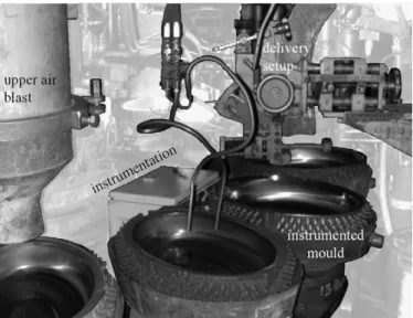
The present industrial process involves sixteen moulds posi-tioned on a carousel and located successively at each stage of the process (see Fig. 2). The rotation cycle time is 48 s. The constraints for the data acquisition system resulting from such industrial context are:
– a high ambient temperature of about 60◦C, – a reduced size,
Table 1
Chemical composition (wt.%) of GX30Cr13 steel (designation NF EN 10027-1)
C Cr Si Mn Ni Fe
0.3 13 0.6 0.9 <0.5 balance
– the impossibility of any physical link with the ground dur-ing the acquisition because of the rotation of the carousel, – the necessity of a quick assembly of the mould after its
furnace preheating.
The moulds are made of GX30Cr13 cast stainless steel (see Table 1). Before machining and polishing, the raw state is ob-tained by sand casting followed by a heat treatment consisting an austenitization, a quenching and a tempering (see Table 2). This heat treatment leads to a tempered martensitic microstruc-ture with a limited hardness compared with traditional mould materials.
2.1. Experimental setup
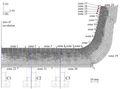
The gauge designed especially for this application is based on the model developed by Dour [25] for the pressure die cast-ing process. It is constituted by a body in which 3 houscast-ings of 0.3 mm diameter have been drilled at 1, 7 and 13 mm from the surface of the gauge. In these housings are stuck the hot junctions of 3 type K thermocouples diameter 0.25 mm (their thinness allows for a very short response time) for the measure-ments of the temperatures required in the inverse method. The temperature measured at 13 mm is imposed, the one at 1 mm is used for the optimization and the one at 7 mm is compared to the calculation to validate the results. The bodies of the gauges are machined from a mould that had been cast especially for that use, in order to be made out of the same materials (composition and solidification structure) than any other one. The gauges are covered with a jacket to protect the thermocouples and placed in an industrial mould in which 3 housings were machined (see Fig. 3).
This so instrumented mould being used in an industrial con-text, an unattended acquisition device has been made up to an-swer to the industrial constraints. An embedded power supply and data storage were required. The inverse method imposes a minimal acquisition frequency and a good accuracy of the measurements. These specifications have been achieved with an industrial automaton National Instrument cFP 2000 realiz-ing the data acquisition at 30 Hz durrealiz-ing the preheatrealiz-ing and a few tens of cycles. The cold junction compensation of the thermocouples has been taken into account by measuring the temperature in the box containing the acquisition material with a PT100 sensor. Each signal providing from a thermocouple has been amplified by an operational amplifier to obtain a resolution lower than 0.1◦C (low cost but time consuming calibration for
each thermocouple).
Fig. 3. Description of the instrumented mould: location of the gauges and ther-mocouples housings.
Fig. 4. Relevance domain of the inverse method [25,27].
2.2. Design of the thermal gauge
The inverse method that has been used in the present study is founded on the thermal quadrupoles formulation [16] (Laplace transformation of the heat conduction equation in one dimen-sion) and the optimization problem is solved using the Beck’s method [20] as described by Broucaret [26].
This method requires two temperature measurements: the first one is imposed as a boundary condition in the direct prob-lem and the second one is used to minimize the differences be-tween experiment and calculation. A relevance diagram (Fig. 4) has been mapped out [25,27] to determine the validity of the results as a function of some dimensionless parameters rele-vant to the acquisition (sampling period dt, distance between the surface and the first measurement location e), to the process (characteristic time of the heat exchange τ , chosen equal to 1 s a priori, corresponding to the duration of the application of the pressure on the gob) and to the mould material (diffusivity κ, 4.9× 10⁻⁶m2s−1for the studied steel). In order to be located
in the middle of the validity domain, it has been retained a dis-tance of 1 mm between the first measurement location and the surface, and a sampling time of 0.03 s.
Table 2
Elaboration, heat treatment and hardness of GX30Cr13 steel
Sand casting Normalization Austenitizing Quenching Tempering Hardness 1600◦C/Ar 880◦C/3 h 1000◦C/8 h Air blast 680◦C/6 h 280 HB/27 HRc
3. Results and discussion
The instrumented mould presented above has been used in the factories of the group Arc International Cookware at Sun-derland (UK) and Châteauroux (France). The results presented here concern the measurements realized at Sunderland. The preheating temperature is about 370◦C and about twenty cycles
are required to stabilize the mean temperature. In a stabilized cycle, the surface temperature varies between 430 and 605◦C.
3.1. Accuracy of the heat flux estimation
From temperature measurement the heat flux and the surface temperature are estimated with the inverse method. The map of relevance (see Fig. 4) showed that the effectiveness of the inverse method is not straightforward. To map out this relevance diagram, the response of the direct problem to a heat flux step function has been used as data of the inverse method. The flux obtained for many values of the inverse method parameters have been compared to the initial heat flux step function to build the different zones of the diagram. The reference [27] shows that using this method, no significant influence of the ntf parameter could be observed in the acceptable zone. We have chosen the parameters of the inverse method (%t) and of the sensors (e) so that it has the best chance to work according to our indications about the process (τ= 1 s).
Nevertheless with ntf = 1, the inverse method is perfectly unstable (the number of future instant, ntf, is the number of consecutive time step used by the Beck’s method to evaluate the least squares error whose minimization allows the estima-tion of the heat flux density value at the next time step). In the acceptable zone, the results of inverse method should not de-pend on the ntf chosen. In the past experiences of Hamasaiid [28], the procedure indeed proposes to choose optimum ntf so that the noise in flux signal is as small as possible, but pro-vided that maximum heat flux density remains in the range of maximum heat flux±noise
2 with lower ntfs. Unluckily this
pro-cedure does not work for us. The effect of ntf is summarized in Fig. 5. We believe that the extremely brief duration of the peak heat flux (about 0.1 s instead of 1 s evaluated a priori due to the quickly decreasing heat flux curve) makes that the operative point on the map of relevance may be translated to-wards under or over evaluation or non-sense zone. Then it can be understood that the peak value depends on ntf. Nevertheless it has no influence on the maximum temperature. Consider-ing that q≈ k%T
%x ≈ 25 40
10−3 = 106 W m−2, a value as high as
6 MW m−2does not seem reasonable.
An other way to evaluate the maximum value of the heat flux density is the normalized approach detailed in [29] if some information about the process are available, as the geometry, the material of the mould, the temperature variation during one
Fig. 5. Influence of the ntf parameters from 2 to 5 (max heat flux density and noise).
cycle and the duration of the heat flux application, supposed to follow a step function. Using the characteristics of the cycle used to show the influence of the ntf parameter (variation of the surface temperature at gauge C3 about 110◦C, duration of the
heat flux density step function of 0.12 s, thickness of the mould and properties of GX30Cr13 steel), one obtains a value about 3.9 MW m−2, what is between the two values found with ntf
equal to 3 and 4 (see Fig. 5). This method is very sensitive to the value of the heat flux duration and a little variation of this parameter allow to obtain the value corresponding to ntf= 3 or
ntf= 4.
We prefer using ntf = 4 that gives lower noise, no overshoot on the time-surface temperature curve and reasonable heat flux density. To improve the results of the inverse method, some modifications of the instrumentation would be necessary, but present technical difficulties: the decrease of the sampling pe-riod, dt, is difficult in the context of unattended acquisition; it may require the diminution of the number of channels. The decrease of the location’s depth of the first thermocouple is fas-tidious due to the proximity of the surface and of the tolerance of the drilling operation.
The time response of the thermocouples, τThC, is also a
pa-rameter that could generate some inaccuracy in the results of the inverse method. The response of the inverse method has been tested as a function of a dimensionless parameter τThC/τ. The sensibility study [25] has shown that the maximal value of the heat flux density is reached if this parameter is lower than 10%. Considering the thermocouple as a first-order sys-tem, its response to a heat flux step function has then an origin slope equal to the ratio qmax/τThC (qmaxis supposed to be the
set point). Assuming that the origin slope is the maximal slope of the time-heat flux density curve, ˙qmax, it could be estimated
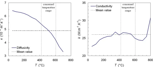
Fig. 6. Evolution of the thermal diffusivity and conductivity of the GX30Cr13 steel with temperature and mean value used for inverse method (Aubert & Duval data).
0.1 s. Then τThC/τ is lower than 10% which is still an
accept-able value.
The deterministic uncertainties on heat flux evaluation de-pends on temperature measurements, thermal properties of the mould and uncertainty in the location of the first thermocou-ple [27]. A normalized analysis of the thermal problem enables the direct estimation of the deterministic errors, as discussed in reference [27], by derivation of the equations of the direct nor-malized problem. The error in the heat flux density dq could be determined from Eq. (5).
dq q = dT %T + dk k + 1 2 dκ κ + qmax k%T dz (5)
where %T is the temperature range (taken to 150◦C
accord-ing to Fig. 8), dT is the error in the temperature measurement (±1.5◦C according to the IEC 584 norm for Class 1 K-type
thermocouples), dk (±1 W m−1K−1) is the error in the thermal
conductivity value assumed to be constant at 26 W m−1K−1,
dκ (±0.5 × 10⁻⁶m2s−1)is the error in the thermal diffusiv-ity value assumed to be constant at 4.9× 10⁻⁶m2s−1, qmaxis
the peak value of the evaluated heat flux density (3.2 MW m−2)
and dz is the inaccuracy in the location of the thermocouple es-timated to±0.055 mm, according to the tolerance in the drilling operation (±0.03 mm) and the accuracy of the location of the thermocouple (0.25 mm diameter) in a greater hole (0.3 mm di-ameter). With these values, the deterministic inaccuracy in the heat flux density estimation was found to be±14.5%. The most influent factors are the diffusivity (5.1%), the location of the thermocouple (4.5%) and the conductivity (3.8%) of the steel, and finally the temperature measurement (1%).
The verifications made above concerning the ntf parameter and the time response of the thermocouples does not allow to validate the results of the inverse method. For that use, the mea-surement of the thermocouple located at 7 mm from the surface of the gauge is compared to the temperature calculated by us-ing the evaluated heat flux density as boundary conditions. The comparison of the temperatures measured and calculated at 13 and 1 mm from the surface are not discussed because they are close to zero, the first one being imposed and the second one
serving as optimization objective. At 7 mm, the error is lower than 20◦C at each gauge (see Fig. 8, Section 3.3), what
corre-sponds to a relative error about 10%. This error is still accept-able because it maximizes the deviation between experiment and calculation over the whole temperature field.
The reasons of such a deviation are of two types. First of all, the assumption is made in the thermal quadrupoles method that the heat transfer is one-dimensional and perpendicular to the surface. This hypothesis does not seem to be of great in-fluence because the same deviation is observable at each gauge, whereas it should be more valid at gauge C1 where heat transfer parallel to the surface should occur considering the symmetry, than at gauge C2 and C3. To compare the velocity of the front matter and the diffusion of the heat in the bulk of the mould, the Peclet number would be useful. From a previous work [1], the velocity of the front matter when the glass flow on the plate surface of the mould has been estimated about 0.25 m s−1. The thickness of the gob is then close to 0.03 m which is also close to the thickness of the mould. Using these values and a diffu-sivity of 4.9× 10⁻⁶m2s−1, one obtains a value of the Peclet
number about 1530. With such a high value, the velocity of the front matter is widely higher as the diffusion of the heat and the heat flux density could be supposed to be applied instanta-neously on the surface of the mould.
The second reason which could explain those deviations is the assumption that the material properties are independent of the temperature. Fig. 6 shows the differences between the ther-mal diffusivity and conductivity of the GX30Cr13 steel and their mean value considered in the range of use of the inverse method. The error made on the thermal conductivity is very weak (lower than 4%), but an error of about 10% exists on the thermal diffusivity for the highest and the lowest temperatures of the range considered.
3.2. Choice of a representative cycle
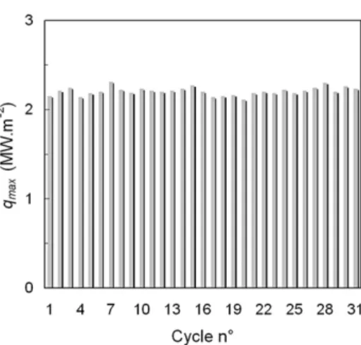
The repeatability of the thermal cycles studied by the de-scribed method is quantified using the maximal and minimal values evaluated for 31 stabilized cycles (see Fig. 7). The peak
Fig. 7. Successive heat flux density peaks in the production steady state at gauge C1.
Table 3
Repeatability of the thermal cycles at gauge C1 (population: 31 cycles) Mean value Standard deviation Maximal value Minimal value qmax, MW m−2 2.20 0.0442 2.31 2.11 qmin, MW m−2 −0.220 0.0213 −0.178 −0.250
mean values are respectively 2.2 MW m−2during pressing and −0.220 MW m−2 during mould cooling. The standard
devia-tion of the maximal flux value is nevertheless only twice the one of the minimal value whereas the mean absolute values are about ten times higher (see Table 3). This is due to the higher sensitivity to the noise for the standard deviation of the weaker values. From this statistical study of the repeatability of the con-secutive cycles, a cycle representative of a standard production process is chosen.
3.3. Upper side temperature surface and heat flux density
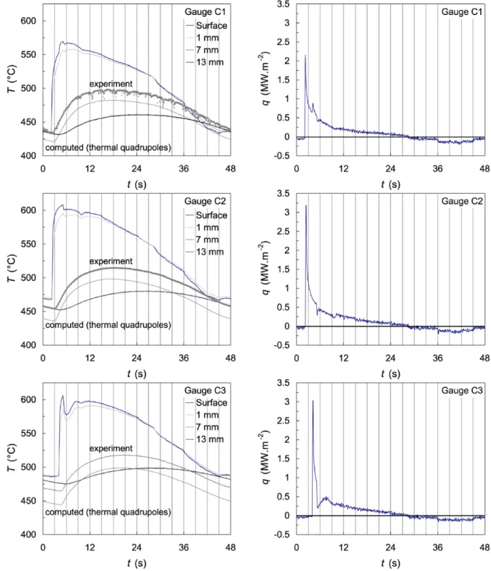
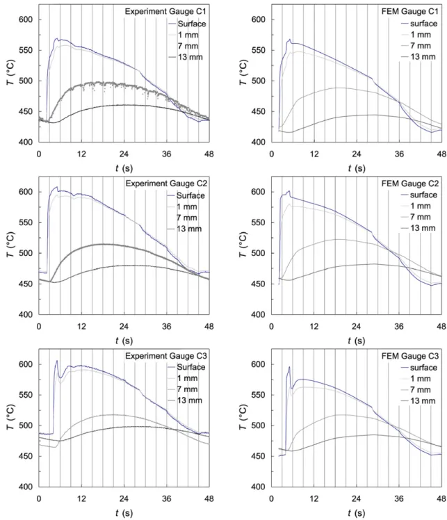
Fig. 8 shows the temperature measurements at the three gauges for the typical average cycle. On the right side of the figure set is shown the heat flux density evaluated for the three gauges. All the key results (Tmin, Tmax, %T , q)are summarized in Table 4.
The maximal temperature at the surface of the mould varies between 565 and 605◦C, depending on the location of the
gauge (see Table 4). It is much lower at gauge C1 (middle of the mould) than at the gauge C2 and C3, which could be explained by a more efficient cooling due to the centering of the upper and lower cooling setups (the minimal temperature is indeed lower as well). No significant differences are observable on the tem-perature amplitude between the minimum and the maximum, but it is slightly lower at gauge C3 (120◦C instead of about 140◦C at gauges C1 and C2). The small difference may be at-tributed to the lower heat absorbed at this location due to the shorter contact time (see Fig. 8). The temperature amplitude at the lower side of the mould is about 25◦C, between 335 and
360◦C.
At the delivery station (n◦1), the temperature increases very
quickly at gauges C1 and C2, but not at gauge C3 because the
latter is not located under the gob. The cooling of the glass generates a thermal contraction having for consequence that the gob leans on its own periphery. The contact is then effec-tive at gauge C2 and non-effeceffec-tive at gauge C1, explaining the higher value of the heat flux density at gauge C2 (3.2 instead of 2.2 MW m−2).
While pressing the glass, the contact pressure increases and a second peak of flux appears at gauge C1 (0.9 MW m−2). This second peak does not exist at gauge C2 because the contact was still fully effective before pressing. A first peak is observable at C3 when the glass flows in front of this gauge. The value of this peak is about the same as at gauge C2 during the waiting time (3.0 MW m−2)but it is not as wide because of a shorter contact
time.
At the end of the pressing stage, the temperature is max-imal at each gauge. Once the upper mould is moved up, the contact pressure is much weaker and the surface temperature begins to decrease. At this time, the behavior of the gauge C3 is sensibly different than the other two. A very quick surface temperature diminution of about 30◦C takes place followed by a slower increase of about 20 ◦C, whereas the temperature de-creases almost regularly at gauges C1 and C2. A possible reason of such a behavior is a detachment between the glass and the mould, more important at the periphery than at the center due to a deformation of the mould when the upper mould moves up. After that, the contact pressure and then the temperature could increase due to a creep of the glass under its own weight or due to the upper air blast. The modeling of this phenomenon would be very difficult because of the number of parameters control-ling it, such as glass mechanical behavior, temperature field in the glass, behavior of the contact between glass and mould . . . The surface temperature of both upper and lower mould could play an important role on the deformation of the glass when the upper tool moves up. Indeed, the separation force between a glass melt and a metallic substrate increases exponentially for mould temperatures above 550◦C whatever the mould material, as shown by Manns et al. [30].
3.4. Comparison between the upper and lower cooling
Fig. 8 shows that the negative heat flux density oscillates nearby two values. The first value occurring during the stages n◦1 (before delivery), 10 (after vacuum take out), 11, 12 and
16 corresponds to a free convection cooling. The second value, lower than the first one, occurs during the stages n◦13, 14 and
15 and corresponds to forced convection while upper air blast cooling.
The mean cooling heat flux density on the upper side of the mould is about −50 kW m−2 for the free convection (a very weak difference exists between each gauge, see Table 4) and between−137 kW m−2and−112 kW m−2for the forced
con-vection (the value is higher at the center of the mould due to the centering of the cooling setup). An important standard de-viation of about 23 kW m−2 is observed on the mean values
above, due to the non-negligible noise existing in the results of the inverse method. From these heat flux density one can esti-mate the convection coefficient between the mould temperature
Fig. 8. Results of the temperature measurements (on left hand) and the inverse method determination of the heat flux density (on right hand) in Sunderland at gauges C1 (top), C2 (middle) and C3 (down). The temperatures computed with thermal quadrupoles (line) and measured (dot) at 7 mm are compared. The vertical rules materialize the transition between two consecutive stations, as numbered on Fig. 1.
Table 4
Characteristics of a representative thermal cycle at gauges C1, C2 and C3
Tmax Tmin %T Peak of flux, MW m−2 qfree qforced hupfree hupforced
◦C ◦C ◦C Station n◦1 Station n◦2 kW m−2 kW m−2 W m−2K−1 W m−2K−1
C1 570. 435. 135. 2.2 0.9 −55. −137. 118. 330.
C2 610. 470. 140. 3.2 – −47. −127. 97.0 285.
Fig. 9. Meshing of the mould for finite element calculation (Abaqus).
and the air at 35◦C. One would find respectively 118, 97 and
89 W m−2K−1 for free convection at gauges C1, C2 and C3
(the mould temperature is respectively of 500, 520 and 540◦C)
and 330, 285 and 241 W m−2K−1for forced convection (the
mould temperature is respectively of 450, 480 and 500◦C).
Qt1→t2=
t2
!
t1
q(t ) dt (6)
The heat density Q+(defined by Eq. (6)) delivered by the gob
to the mould during one stabilized cycle (see Table 5) is larger than the heat density Q− absorbed by convection on the
up-per side of the mould during the same stabilized cycle. This demonstrates the importance of the lower side cooling, twice higher as the upper side one. This could be explained by the duration of the cooling (during the whole cycle on the lower side, but only between vacuum take out and delivery on the up-per side), and the presence of cooling fins on the lower side of the mould. The convection coefficient on the lower side could be estimated considering the heat quantity Q++ Q−to be
ab-sorbed by convection at the lower side during a cycle (48 s) to obtain an equilibrated heat balance. Considering a lower side mould temperature of about 310◦C and an ambient tempera-ture of 35◦C, the values estimated are respectively of 332, 408
and 320 W m−2K−1at gauges C1, C2 and C3. These values are
sensibly higher to the ones estimated for forced convection on the upper side, but this difference is understandable due to the presence of cooling fins.
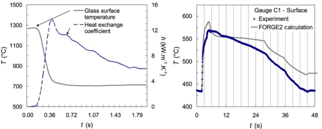
4. Application to finite element calculation 4.1. Temperature field in the whole mould
The experimental results described above are of great inter-est for the calculation of the thermo-mechanical loading
in-Table 5
Lower side convection coefficient estimated at gauges C1, C2 and C3 (Tmould=
310◦C; Tair= 35◦C; tcycle= 48 s)
Q+ Q− Q++ Q− hlowforced habaqus
MJ m−2 MJ m−2 MJ m−2 W m−2K−1 W m−2K−1
C1 6.30 −1.92 4.38 332. 560. C2 7.13 −1.74 5.39 408. 180. C3 5.89 −1.66 4.23 320. 160.
side the whole bulk of the mould. A weak coupled thermo-mechanical calculation has been realized with the finite element software ABAQUS. In a first approach, the mould was sup-posed to be axis-symmetric with a projected working surface equivalent to the elliptical geometry. The meshing was consti-tuted of 4834 quadrangular elements and 5404 nodes (linear interpolation of the temperature), see Fig. 9. The uniform initial condition corresponds to the preheating temperature (370◦C).
The boundary conditions applied on the meshing are those es-timated by inverse method from the temperature measurement in production conditions. Two kinds of boundary conditions are applied: heat flux on the working surface and convection coef-ficient on the external sides.
The work surface has been divided into 17 faces. On the first one, the heat flux density estimated at gauge C1 is applied. On the second one, the heat flux density estimated at gauge C2 is applied. On the third face, the heat flux density estimated at gauge C2 is applied with a time lag in order to simulate the creeping of the gob under its own weight before pressing. On the fourth face, the heat flux density estimated at gauge C3 is applied. On the faces 5 to 17, the heat flux density estimated at gauge C3 is applied with a time lag in order to take into ac-count the progression of the glass front while forming. The size of the different faces and the value of each time lag have been determined from the results of a simulation with FORGE2 FEM
Fig. 10. Comparison between the measured temperature (on left hand) and the temperatures computed with finite element method (on right hand) in Sunderland at gauges C1 (top), C2 (middle) and C3 (down). The vertical rules materialize the transition between two consecutive stations, as numbered on Fig. 1.
package of the glass flow during the glass pressing process. A time lag corresponds to a time step of this calculation, and the size of the corresponding face is equal to the progression of the front matter during this step. The initial and boundary con-ditions used in this previous glass flow simulation were taken from the literature (time dependent heat exchange coefficient according to the results of the reference [17]) and does not match exactly our processing conditions. Nevertheless, the cin-ematic of the press was imposed, and even if the stress results may be discussable, the movement of the front matter should be well described. The details of this simulation are available in a previous paper [1].
The external surface of the mould has been divided into 4 faces. The first three are located under each gauge and the convection coefficients applied have been estimated previously from temperature measurement (see Table 5). On the last face corresponding to the lateral external side of the mould, a con-vection coefficient of 110 W m−2K−1has been applied, as es-timated above for free convection (see Table 4).
Sixty cycles have been simulated with these boundary condi-tions in order to obtain a stabilization of the mean temperature. A significant difference between the measured and calculated stabilized temperature has been observed due to the one di-mensional assumption used to determine the values from the
Fig. 11. FORGE2 calculation: boundary conditions during waiting time before pressing (on left hand) and comparison of the surface temperature calculated and estimated by inverse method (on right hand).
experimental data, the ratio between heat transfers parallel and perpendicular to the surface increasing with the distance of the surface. The values of the convection coefficient applied under each gauge have then been optimized in order to min-imize this difference. The optmin-imized values are respectively of 560, 180 and 160 W m−2K−1 instead of respectively 332, 408 and 320 W m−2K−1. After optimization, the differences between experience and simulation are very weak at each com-parison points (measured bulk temperatures, estimated upper surface temperature and measured lower surface temperature). As shown in Fig. 10, the differences between measurements and simulation are very weak (less than 20◦C at each
compar-ison point over the whole cycle). The surface temperature is very well evaluated. The temperature dependence of the ther-mal properties of the steel has been taken into account in the finite element calculation leading to a better agreement with the experimental data at 7 mm with finite element (Fig. 10), than with thermal quadrupole (Fig. 8).
4.2. Validation of the simulation of the glass forming by pressing
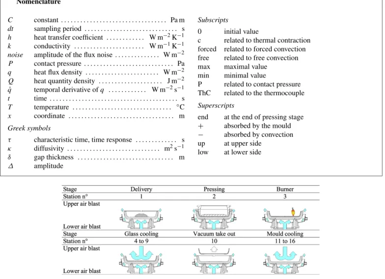
A simulation of the pressing process (see [1] for details) has been realized with the finite element software FORGE2. The simplified thermal boundary conditions applied on this fully coupled thermo-mechanical calculation in the gob and in the lower mould were a heat exchange coefficient and eventually a time dependent opposite surface temperature (the boundary conditions described further could differ from those presented in [1], due to the availability of experimental data).
During waiting time before pressing, the heat exchange co-efficient and the opposite temperature (corresponding to gob surface temperature) applied are function of time as described in Fig. 11. The temperature of the gob surface is computed independently by imposing the heat flux density estimated by inverse method on the glass with a one-dimensional finite dif-ferences calculation (the heat exchange coefficient can then be estimated). During the pressing stage and the glass cooling stages, the heat transfer coefficient is supposed to be constant
(7 kW m−1K−1 for pressing and 500 W m−1K−1 for glass
cooling) and the opposite temperature is the one calculated at the surface of the gob mesh. The initial condition results from the independent gob temperature simulation during the waiting time. During mould cooling, the values of the heat exchange co-efficient and opposite temperature are those estimated at gauge C1 (118 W m−1K−1 for free convection, 330 W m−1K−1for forced convection and ambient temperature of 35◦C).
The results presented in Fig. 11 compare the surface tem-perature calculated with FORGE2 and the surface temtem-perature estimated at gauge C1 with the inverse method. It can be ob-served a good description of the evolution of the temperature during waiting time and pressing, as well as while cooling the mould surface by free or forced convection, even if a significant over evaluation exists. During the cooling of the glass part, the evolution of the temperature is not realistically described by the hypothesis of constant heat transfer coefficient explaining par-tially the later over evaluation of the surface temperature. This error may be due to the very complex behavior of the contact between the glass and the mould after pressing as discussed at the end of Section 3.3.
5. Conclusion
The results of an investigation of the heat flux density ex-tracted from a gob by glass pressing in a mould made out of martensitic stainless steel was presented. With this aim in view, an instrumentation as non-intrusive as possible has been devel-oped to measure temperatures in the bulk of the mould in nor-mal production conditions. This instrumentation is composed of three gauges, each allowing temperature measurements at 1, 7 and 13 mm from the surface of the mould. An inverse method based on the thermal quadrupoles and the Beck’s optimization method has been used to exploit these measurements and eval-uate the heat flux density absorbed as well as the temperature at the surface of the mould. The study of the difference between each gauge during a representative cycle shows the influence of the production stages, the heterogeneity and the complexity of the thermal loadings at the surface of the mould. The
pre-dominance of the lower air blast cooling over the upper one has been demonstrated comparing the heat quantities delivered by the gob and absorbed by convection on the upper side of the mould. This observation justifies the presence of cooling fins on the lower surface. The quality of these results has been discussed in terms of the validity of the hypothesis and of the in-fluence of the intrinsic parameters of the inverse method and of the instrumentation. The use of the heat flux density evaluated as boundary conditions in a finite element calculation allow to calculate with a very good accuracy the evolution of the tem-perature field in the whole bulk of the mould. It has also been shown that the hypothesis of constant heat transfer coefficient is not sufficient to describe properly the evolution of the surface temperature of the mould, especially during the glass part cool-ing stages. This also reflects the complexity of the glass/mould interface as deduced from our measurements.
Acknowledgements
The authors greatly acknowledge the financial support of this work by Arc International Cookware, Aubert & Duval and Saint-Gobain SEVA. This study would not have been carried out without the participation of the production teams of the manufacturing plants of Châteauroux and Sunderland. Special thanks are expressed to M. Daniel Deletang.
References
[1] G. Dusserre, F. Schmidt, G. Dour, G. Bernhart, Thermo-mechanical stresses in cast steel dies during glass pressing process, J. Mater. Process. Tech. 162–163 (2005) 484–491.
[2] K. Pöting, Future trends in hollow glass production, in: Proceedings of the Colloquium on Modelling of Glass Forming Processes, Valenciennes, France, 1998, pp. 9–16.
[3] J. Linhart, S. Linhart, Temperature measurement in the glass melt, Glass Technol. 43 (5) (October 2002) 198–202.
[4] H. Rawson, Comments on “Heat transfer modelling of the parison form-ing in glass manufacturform-ing” by K. Storck, D. Loyd, B. Augustsson (Glass Technol. 39 (1998), 210–216, Glass Technol. 40 (1997) 97–98.
[5] D. Höhne, B. Pitschel, M. Merkwitz, R. Lobig, Measurement and math-ematical modeling of the heat transfer in the glass forming process, in consideration of the heat transfer coefficients and radiation influences, Glass Sci. Technol. 76 (2003) 309–317.
[6] K. Storck, D. Loyd, B. Augustsson, Heat transfer modelling of the parison forming in glass manufacturing, Glass Technol. 39 (1998) 210–216. [7] T. Loulou, R. Abou-Khachfe, J.P. Bardon, Estimation de la résistance
ther-mique de contact durant la solidification du verre, Int. J. Therm. Sci. 38 (1999) 984–998.
[8] R. Abou Khachfe, Estimation de la résistance thermique de contact entre un métal et une pastille de verre, Master’s thesis, Université de Nantes, France, 1997.
[9] R. Viskanta, J. Lim, Analysis of heat transfer during glass forming, Glass Sci. Technol. 74 (2001) 341–352.
[10] S.K. Pchelyakov, Y.A. Guloyan, Heat transfer at the glass mould interface, Glass Ceram. 42 (1985) 400–403.
[11] G. Keijts, K. van der Werff, Heat transfer in glass container production during the final blow, Glass Technol. 42 (2001) 104–108.
[12] S.V. Tarakanov, V.K. Leko, O.V. Mazurin, Some problems of precise mea-surements of heat transfer coefficients in glass melts. I: Meamea-surements of effective conductivity, Glass Sci. Technol. 68 (1995) 301–311.
[13] B. Sawaf, M.N. Ozisik, Y. Jarny, An inverse analysis to estimate lin-early temperature dependent thermal conductivity components and heat capacity of an orthotropic medium, Int. J. Heat Mass Transfer 38 (1995) 3005–3010.
[14] R. Abou Khachfe, Y. Jarny, Résolution numérique d’un problème d’esti-mation de source thermodépendante dans un domaine bidimensionnel, in: Congrès SFT99, Arcachon, France, 1999.
[15] R. Abou Khachfe, Y. Jarny, Determination of heat sources and heat trans-fer coefficient for two-dimensional heat flow: Numerical and experimental study, Int. J. Heat Mass Transfer 44 (2001) 1309–1322.
[16] D. Maillet, S. André, J.C. Batsale, A. Degiovanni, C. Moyne, Thermal Quadrupoles – Solving the Heat Equation through Integral Transforms, John Wiley and Sons, New York, 2000.
[17] P. Moreau, S. Grégoire, D. Lochegnies, Méthodologie expérimentale pour la détermination du coefficient de transfert thermique à l’interface verre/outil, Verre 9 (2003) 24–27.
[18] R. Abou Khachfe, Y. Jarny, Numerical solution of 2-d nonlinear heat con-duction problems using finite-element techniques, Numer. Heat Transfer B – Fund. 37 (2000) 45–68.
[19] Y. Jarny, M.N. Ozisik, J.P. Bardon, A general optimization method using adjoint equation for solving multidimensional inverse heat conduction, Int. J. Heat Mass. Transfer 34 (1991) 2911–2919.
[20] J.V. Beck, K.J. Arnold, Parameter Estimation in Engineering and Science, John Wiley and Sons, New York, 1977.
[21] R. Abou Khachfe, Résolution numérique de problèmes inverses 2D non linéaires de conduction de la chaleur par la méthode des éléments finis et l’algorithme du gradient conjugué – Validation expérimentale, PhD thesis, Université de Nantes, France, 2000.
[22] D.A. McGraw, Transfer of heat in glass during forming, J. Am. Ceram. Soc. 44 (1961) 353–363.
[23] E. Brauns, J. Patyn, E. Wiersema, A. Skerath, Finite element calculation of thermomechanical stresses in candidate ceramic components for press and blow moulds, Glass Technol. 40 (1999) 58–64.
[24] S.P. Jones, P. Basnett, G.C. Parker, BGIRA research report n◦29, British Glass, Sheffield, 1966.
[25] G. Dour, M. Dargusch, C. Davidson, A. Nef, Development of a non-intrusive heat transfer coefficient gauge and its application to high pressure die casting: Effect of the process parameters, J. Mater. Process. Tech. 169 (2005) 223–233.
[26] S. Broucaret, A. Michrafy, G. Dour, Heat transfer and thermo-mechanical stresses in a gravity casting die: Influence of process parameters, J. Mater. Process. Tech. 110 (2001) 211–217.
[27] G. Dour, M. Dargusch, C. Davidson, Recommendations and guidelines for the performance of accurate heat transfer measurements in rapid forming processes, Int. J. Heat Mass Transfer 49 (2006) 1773–1789.
[28] H. Hamasaiid, Etude des phénomènes thermiques à l’interface pièce/outil en fonderie, PhD thesis, Université Toulouse 3 Paul Sabatier, France, 2007.
[29] G. Dour, Thermal stresses and distortion in die casting processes: a new normalized approach, Modelling Simul. Mater. Sci. Eng. 9 (2001) 399– 413.
[30] P. Manns, W. Döll, G. Kleer, Glass in contact with mould materials for container production, Glass Sci. Technol. 68 (1995) 389–399.
![Fig. 4. Relevance domain of the inverse method [25,27].](https://thumb-eu.123doks.com/thumbv2/123doknet/12580281.346713/5.892.467.843.435.694/fig-relevance-domain-inverse-method.webp)