HAL Id: inria-00549856
https://hal.inria.fr/inria-00549856
Submitted on 13 Jan 2020
HAL is a multi-disciplinary open access
archive for the deposit and dissemination of
sci-entific research documents, whether they are
pub-lished or not. The documents may come from
teaching and research institutions in France or
abroad, or from public or private research centers.
L’archive ouverte pluridisciplinaire HAL, est
destinée au dépôt et à la diffusion de documents
scientifiques de niveau recherche, publiés ou non,
émanant des établissements d’enseignement et de
recherche français ou étrangers, des laboratoires
publics ou privés.
Rules by Navigating in a Lattice of OLAP Views
Pierre Allard, Sébastien Ferré, Olivier Ridoux
To cite this version:
Pierre Allard, Sébastien Ferré, Olivier Ridoux. Discovering Functional Dependencies and Association
Rules by Navigating in a Lattice of OLAP Views. Concept Lattices and Their Applications, Oct 2010,
Sevilla, Spain. pp.199-210. �inria-00549856�
Association Rules by Navigating in a Lattice of
OLAP Views
Pierre Allard⋆, S´ebastien Ferr´e, and Olivier Ridoux
IRISA, Universit´e de Rennes 1, Campus de Beaulieu 35042 Rennes Cedex, France
[email protected], [email protected], [email protected]
Abstract. Discovering dependencies in data is a well-know problem in database theory. The most common rules are Functional Dependencies (FDs), Conditional Functional Dependencies (CFDs) and Association Rules (ARs). Many tools can display those rules as lists, but those lists are often too long for inspection by users. We propose a new way to display and navigate through those rules. Display is based on On-Line Analytical Processing (OLAP), and organize a set of rules as a cube, where dimensions correspond to the premises of rules. Cubes reflect the hierarchy that exists between FDs, CFDs and ARs. Navigation is based on a lattice, where nodes are OLAP views, and edges are OLAP naviga-tion links, and guides users from cube to cube. We present an illustrative example with the help of our prototype.
Keywords: Functional Dependencies, Association Rules, FCA, OLAP, Navigation
1
Introduction
Discovering dependencies in data is a well-know problem in database theory. Using dependency rules can help to prevent redundancy, to optimize queries and to avoid update errors. There are many softwares for computing dependency rules in a table. They generally provide the rules as a list. The main problem for users is to find the relevant information in those lists. Therefore, users need tools to navigate among them, and to check them. In this paper, we present how to create views over a table, such that users are able to visualize rules. Then we present how to guide users to navigate from a view to another.
We study the discovery of the following kinds of rules. Functional Depen-dencies (FDs) [7] are depenDepen-dencies that are valid on entire tables. Conditional Functional Dependencies (CFDs) [8] are FDs that apply on a subset of a table.
Association Rules (ARs) [1, 19] are dependencies that apply for particular values of some attributes. An AR can be exact or approximate. Medina and Nourine [14] present the hierarchy that exists between FDs, CFDs and ARs [19, 16], with the help of Formal Concept Analysis (FCA) [10]. Those rules are always in the form premises - conclusion.
The number of rules extracted from a table is often too high. We must there-fore provide to the user synthetic views showing a subset of rules. In a number of works, those views are defined by premises and conclusion [5]. Most works is about rule visualization, rather than on which view to choose [18, 5]. In this paper, we use another database tool, On-Line Analytical Processing (OLAP) to create and navigate between views. OLAP [6] is often used in Business Intel-ligence environments. It allows users to aggregate (e.g. sum, average) data at several granularity levels, without knowing a query langage, and to display re-sults in charts. We are interested in OLAP because of the OLAP data structure: cubes, i.e. multidimensional representations of data. A cube is defined by a mea-sure (the values, e.g. the sales) and a set of dimensions (e.g., by month). In this paper, we show that dependency rules can be found visually in a cube, because of the similarity of the form premises - conclusion of the dependency rules and the form dimensions - measure of the cubes. Several papers use lattices along OLAP, often for supporting the precomputation of OLAP cubes [17]. Casali et al. [4] show a method to organize cubes in a closed cube lattice, to improve the computation of aggregations. Medina and Nourine [15] create a concept lat-tice, where each concept is a set of dimensions. Their work allows to discover dependency rules from the lattice.
The number of different cubes can be too high to vizualize them all. There-fore, users need tools to navigate from cube to cube. We relate this work to Logical Information Systems (LIS) [9]. LIS allow users to browse a context (in the sense of FCA) by navigating from concept to concept. The most common OLAP navigation links allow to add or remove a dimension, or to change the granularity level of a dimension. We show that the OLAP navigation links can be used in addition to LIS navigation links.
The main motivation for this paper is to demonstrate that OLAP offers a good support to display and navigate the dependency rules. First we introduce the concepts and definitions, along with illustrative examples, that are needed in our study (Section 2). Next we present how to visualize dependency rules in a cube (Section 3). Then we present the navigation part, to navigate from cube to cube (Section 4). Finally, we detail an example of navigation (Section 5), and conclude (Section 6).
2
Background and Definitions
A relation, as in databases, is comparable to a many-valued context. A relation schema R is defined by a set of attributes Attr(R). The domain of each attribute A ∈ Attr(R) is denoted by Dom(A). An instance of a relation schema R, a relation r, is a set of transactions. Each transaction t maps a value to each
re Date Seller P rice P roduct N umber Store
t1 01/09 John 179 AT V 2 Rennes
t2 01/16 Abby 159 AT V 1 St-M alo
t3 01/16 Abby 119 BM X 3 Quimper
t4 01/23 Abby 119 BM X 3 Brest
t5 01/23 Abby 119 P ants 7 N antes
t6 01/23 Jim 29 Shoes 4 Angers
t7 02/06 Bob 59 Shoes 4 Angers
t8 02/13 John 15 Balloon 20 Laval
t9 02/20 Jim 129 Skates 5 Lorient
t0 02/27 Bob 79 Sneakers 6 St-Brieuc
Table 1. An example relation re, instance of Re, with
Attr(Re) = {Date, Seller, P rice, P roduct, N umber, Store}.
attribute. The notation t[X] represents the values of the transaction t, for the attribute sequence X. Table 2 shows the example relation re, which is an instance
of Re and contains a set of sales. This relation is extracted from [14]. We only
changed the labels of values to render the relation less abstract and to add granularity levels (used in Section 3.2).
In this article, we only study dependency rules whose conclusion has a single attribute. A Functional Dependency (FD) [7] expresses the fact that some at-tribute (the conclusion) of a relation is determined by a set of other atat-tributes (the premises). We only study exact FDs and not Approximate Dependencies [13].
A FD X → Y , with X ⊆ Attr(R) and Y ∈ Attr(R), is valid on r if ∀t1, t2∈
r, (t1[X] = t2[X]) ⇒ (t1[Y ] = t2[Y ]).
A Conditional Functional Dependency (CFDs) [8, 14] is defined by a pair ϕ = (X → Y, Tp), where X → Y is a standard FD, and Tp⊆ r is a set of patterns
called tableau. ϕ is valid if ∀t1, t2 ∈ Tp, (t1[X] = t2[X]) ⇒ (t1[Y ] = t2[Y ]).
For example, ϕe= (P roduct → N umber, {( , , , BM X, , ), (01/23, , , , , )})
represents the FD P roduct → N umber restricted to the subset of sales where P roduct = BM X or Date = 01/23, whatever the other attribute values are. The notation represents any value of the corresponding attribute.
An Association Rule (AR) [1] expresses the fact that the value of an attribute (the conclusion) is determined by the values of other attributes (the premises). An AR d is denoted by d = X → Y , where X = ((A1= b1) ∧ . . . ∧ (Ap= bp) and
Y = (Aq = bq)), with Ai ∈ Attr(R) and bi ∈ Dom(Ai). The support of an AR
is the number of transactions matching both the premises and the conclusion. The confidence conf (d, r) of d is the ratio of transactions respecting the AR. When conf (d, r) = 1, the AR is said exact. Traditionally, users are interested in exact ARs Approximate ARs (AAR) [19, 16] are ARs having a confidence < 1.
Huhtala et al. [12] use the notion of X-complete relation [3] and a closure operator to find FDs. A relation r is X-complete if ∀t1, t2 ∈ r, t1[X] = t2[X].
complete. Applying a closure operator, it is possible to form FDs. The X-complete partition lattice consists of concepts which represent the partitions, ordered by FD and labelled to find CFD. Medina and Nourine [15] show the X-complete partition lattice of a relation. Each concept shows the set of attributes X and a tableau Tp, such that the transactions of Tpare X-complete. Each edge
(X, Y ) is labelled by a tableau Tp, such that r |= (X → Y, Tp). The benefits of
this lattice is that it gives a synthetic view of the CFDs and ARs of a relation. Codd introduced the concept of On-Line Analytical Processing (OLAP) [6]. Originally, OLAP is designed for Business Intelligence. Indeed, it allows users to aggregate quickly large sets of values, depending on study axes, and to cre-ate charts. OLAP users do not need to know a specific language to query the database. Data contained in OLAP warehouses are multidimensionally struc-tured. Each fact of the table contains a measure value (the data that will be aggregated), and dimension values for each study axe. For example, the sale amounts (measure) by store, and by date (dimensions). Each dimension can have several levels of granularity. For example, the date dimension can be expressed by day, month or year. An OLAP table is represented by a cube, reflecting the multidimentional structure. OLAP users can trigger navigation links to navigate from cube to cube.
The main problem of OLAP is that the navigation space is restricted by the starting cube. For instance, OLAP users can neither change the measure (e.g., set the store as measure), nor add a dimension (e.g., add a seller dimension). Therefore, a request to the database administrator is necessary to extract a new starting cube. In [2], authors present an OLAP model to overcome this limitation. The measure is considered as a special dimension, and can be exchanged with the help of a additional navigation links. In recent years, works on OLAP allowed it to scale to large databases, especially with the help of precomputation [17]. In this paper, we focus on the OLAP concepts of cube structure, granularity levels and navigation links. We do not consider here aspects related to the display of charts, and the precomputation of views. We define cube schemas and cubes. Definition 1 (Cube Schema, Cube). A cube schema C is defind by a tuple of dimensions, Dim(C) = (A1, . . . , Ap), and a measure, M eas(C) = Aq. A cubec
that is an instance ofC is defined by a function f : Dom(A1)×. . .×Dom(Ap) →
Dom(Aq). This total function allows to access the contents of each cell of the
cube.
We study OLAP because of the representation of a cube. Indeed, each cell of a cube represents a transaction or a set of transactions, ordered in a cube structure. The mining of FD implies to check, for any combination of the premise values, if the conclusion value is the same. The cube structure presents all combinations of premise values.
3
Relation projections
In our mining of dependency rules, we introduced OLAP, because of the simi-larity between the form (premises - conclusion) of the dependency rules, and the
Date
01/09 01/16 01/23 02/06 02/13 02/20 02/27 {{John}} {{Abby, Abby}} {{Abby, Jim}} {{Bob}} {{John}} {{Jim}} {{Bob}} Table 2.The projection ce of re, with Dim(ce) = (Date) and M eas(ce) = Seller.
form (dimensions - measure) of the cubes. In order to extract rules from a cube, we need to project the relation into a cube.
3.1 Projection of a Relation into a Cube
A cube actually forms a particular view of a relation. The main difference is the distinction between dimensions and the measure, which does not exist in a relation. We use this distinction to form dependency rules. For each transaction of the relation, we place the measure value in the cell of the cube corresponding to the dimension values. The measure values of each cell are usually aggregated. In our study, we retain the measure values as a multiset, because we are interested in dependency rules. Therefore, a cube is defined by a total function f that returns for each cell a multiset of measure values. Thereafter, we consider that an attribute has the same domain in the relation schema and the cube schema. Definition 2 (Projection of a relation into a cube). Let r be a relation with attributes Attr(r). A cube c is obtained by the projection of the relation r on dimensions Dim(c) = (D1, . . . , Dp) such that Di ∈ Attr(r) for i ∈ [1, p],
and on the measure M eas(c) = Dq ∈ Attr(r). The domain of the dimensions
are the same as the domain of their corresponding attributes in the relation. The domain of the measureM eas(Dq) is made of multisets over Dom(Dq). The
following function f maps each cell of the cube to a multiset of values from the relation:
f (b0, . . . , bp) = {{bq|t ∈ r, (t[D1] = b0) ∧ . . . ∧ (t[Dp] = bp) ∧ (t[Dq] = bq)}}.
For example, Table 3.1 shows the projection ce of re, where the dimensions
are Dim(ce) = (Date) and the measure is M eas(ce) = Seller. The result of the
projection is like a traditional OLAP cube, but data are not aggregated. The advantages are that any kind of value can be studied (e.g. strings), and there is no information loss for rule visualization.
Now we show that FDs, CFDs and exact ARs can be visually found in the relation projection (cube), and that the hierarchy between those rules is re-spected. Indeed, a cell of the cube at coordinates D1= d1, . . . , Dp= dpcontains
the multiset of values taken by the attribute Dq, in all transactions such that
D1 = d1, . . . , Dp = dp. The definition of exact ARs D1 = d1 ∧ . . . ∧ Dp =
dp → Dq = dq is that for any transaction such that D1 = d1∧ . . . ∧ Dp = dp,
then Dq = dq. Then, in this cell, if there is only one value in the multiset (e.g.
Seller
John Abby Jim Bob
01/09 {{AT V }} 01/16 {{AT V, BM X}} 01/23 {{BM X, P ants}} {{Shoes}} Date 02/06 {{Shoes}} 02/13 {{Balloon}} 02/20 {{Skates}} 02/27 {{Sneakers}}
Table 3. The projection ce of re, with Dim(ce) = (Seller, Date) and M eas(ce) =
P roduct.
Sebastien¿ Il nous fallait trouver un cube a deux dimensions pour que ca soit plus concret. J’ai donc cherche un cube a deux dimensions ou je pouvais apercevoir une cellule avec 2 valeurs egales ({{Abby, Abby}}) et une cellule avec 2 valeurs differ-entes ({Abby, Bob}}). J’ai cherche avec toutes les combinaisons possibles, et je n’ai pas trouve. Il faudra donc choisir entre un exemple sur un cube digne de ce nom et un cube ou on voit les multi-ensembles...
Pierre¿ et si tu aggreges par mois ?
(e.g. {{a, a, b}}), the AR is approximate. Thus, the cube is a synthetic view of all the possible ARs following the dimensions and measure.
Theorem 1 (Association Rule in the cube). Let d = (D1= b1)∧. . .∧(Dp=
bp) → (Dq = bq) be an AR, and c be a cube with Dim(c) = (D1, . . . , Dp),
M eas(c) = Dq, andf be the projection function of c. The support of this rule is
equal to the number of elements that have valuebq in the cell ofc at coordinates
(b1, . . . , bp):
sup(d, r) = k{{b|b ∈ f (b1, . . . , bp) ∧ b = bq}}k.
The confidence is equal to the ratio of elementsbq on all the elements on the
cell at coordinates (b1, . . . , bp):
conf (d, r) = sup(d, r) kf (b1, . . . , bp)k
.
There exists a hierarchy between FDs, CFDs and ARs [14, 15]. Indeed, a FD X → Y is equivalent to a CFD (X → Y, Tp) where Tp = r (i.e. Tp selects all
transactions in the relation). Moreover, a CFD is equivalent to a set of ARs. For example, the CFD (Date → Seller, {(01/09, , , , , ), (01/23, , , , , )}) is equivalent to the set of ARs {(Date = 01/09 → Seller = John), (Date = 01/23 → Seller = Abby)}. There is a complete hierarchy between FDs, CFDs and ARs. Following the same reasoning as for ARs, it is possible to find CFDs and FDs in a cube. Let c be a cube. If each cell of c contains one or zero element in its multiset, then the FD Dim(c) → M eas(c) is valid. That can be justified by the fact that a FD can be decomposed into a set of ARs, from [14].
Theorem 2 (Functional Dependency in the cube). Let D1, . . . , Dp →
Dq be an FD in a relation r, and c be a cube with Dim(c) = (D1, . . . , Dp),
M eas(c) = Dq,f be the projection function of c. This FD is valid in r iff, in c:
∀(b1, . . . , bp) ∈ (Dom(D1) × . . . × Dom(Dp)), ∀v1, v2∈ f (b1, . . . , bp), v1= v2.
The definition of a CFD in the cube is between the definition of an AR and a FD. If each cell in a subset of the cube (e.g. a line or a square subset) contains one or zero element in its multiset, then there is a valid CFD, whose pattern tableau covers the subset of the cube. The hierarchy established by [14] is here confirmed, according to the number of cells with one or zero element.
For example, Table 3.1 shows dependency rules. We note that each cell except {{Abby, Jim}} has one distinct value. This implies that there are ARs at those cells (e.g. Date = 01/06 → Seller = Abby), and a CFD whose pattern covers those cells ((Date → Seller, {(01/09, , , , , ), . . .})). On the contrary, no FD can be found from this view.
3.2 Granularity Levels
A major strength of OLAP is the definition of taxonomies on the dimensions. Indeed, the dimension values are hierarchically organized, according to several levels of granularity. In traditional OLAP, an aggregation function can synthesize the grouped data, using a function (e.g., sum, average, count). Han and Fu [11] show methods to find ARs at several levels of granularity. It is interesting to see how ARs, then FDs, can be seen in a cube with taxonomies. We now formalize the taxonomy of dimensions.
Definition 3 (Dimension taxonomy). Let D be a dimension. This dimen-sion, at granularity level δ, is denoted by D ∼ δ. A dimension taxonomy on D is defined by a set of n ordered levels ∆ = {1, . . . , n} and a set of rules bi ⊑ bj,
with bi ∈ Dom(D ∼ i), bj ∈ Dom(D ∼ j), and j = i − 1. The levels form
a partition of the dimension values, i.e., Dom(D) = ∪i∈nDom(D ∼ i) and
∀i, j ∈ 1 . . . n, Dom(D ∼ i) ∩ Dom(D ∼ j) = ∅. To get a more concise notation, a dimension without taxonomy keeps its old notation.
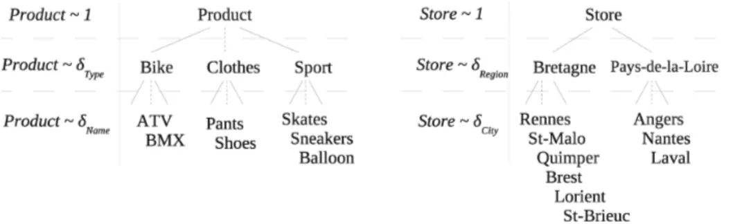
Figure 3.2 presents a dimension taxonomy for the P roduct and Store dimen-sions. A product can be represented by its type, and a store by its region. The definition of a cube schema is not modified. We redefine a projection function from a relation to a cube, using taxonomies.
Definition 4 (Projection of a relation in a cube with taxonomies). Let r be a relation with attributes Attr(r). A cube c is the projection of the relation with taxonomies, on dimensions Dim(c) = (D1, . . . , Dp) such that Di∈ Attr(r),
and a set of levels(δ1, . . . , δp) for each dimension, and a measure M eas(c) = Dq,
withDq∈ Attr(r) and δq a level ofDq. The domains of elements ofDim(c) are
Fig. 1.The dimension taxonomies of P roduct and Store. Date ∼ δmonth 10/01 10/02 Seller John {{2}} {{20}} Abby {{1, 3, 3, 7}} Jim {{4}} {{5}} Bob {{4}} {{6}}
Table 4. The projection cet of re, with the dimensions Dim(cet) = (Date ∼
δmonth, Seller) and the measure M eas(c) = N umber.
domain ofM eas(c) is equivalent to the multiset of Dom(Dq ∼ δq). The following
function f maps each cell of the cube to a multiset of values from the relation: f (b′ 1, . . . , b ′ p) = {{b ′ q|t ∈ r, ∀k ∈ 1 . . . p, q, (t[Dk] = bk∧ bk ⊑ b′k)}}.
This definition allows users to create new cubes, at several granularity levels. This implies that more dependency rules can be extracted from the relation. For instance, Table 3.2 shows the result of the projection of re in cet, with the
dimensions Dim(cet) = (Date ∼ δmonth, Seller) and the measure M eas(cet) =
N umber. We can then deduce that the CFD ϕ2 = (Date ∼ δmonth∧ Seller →
N umber, {( , John, , , , ), ( , Jim, , , , )}) is valid on re.
4
Navigation
In the previous section we show that a projection of a relation into a cube allows to see the FDs, CFDs and ARs, following the dimensions and the measure of the cube. To give access to all dependency rules, we need to give access to cubes for all dimension combinations, granularity levels, and measures.
To navigate from cube to cube, changing granularity levels, adding or remov-ing dimensions, we use OLAP navigation links. Traditionally, OLAP systems do not have an add navigation link, to add a dimension (because of the initial cube problem). We add this navigation link. The set of navigation links is:
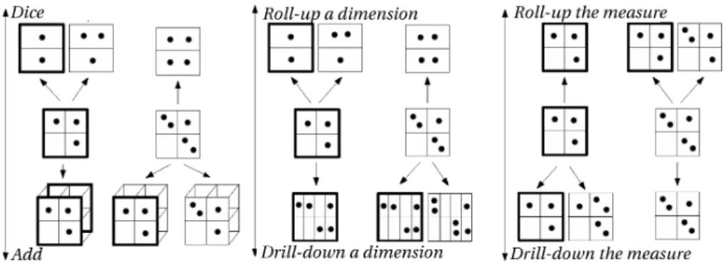
Fig. 2. The several OLAP navigation links. A cell with one or zero point means an exact AR. A cell with two points mean an approximate AR. The bold cubes mean the FD is true.
Roll-up(dimension / measure) Traditionnaly, a roll-up changes the granularity level of a dimension. Our choice is to consider the measure as a special dimension, then a roll-up can here be used on the measure. Formally, a roll-upon D ∼ δi will modify it into D ∼ (δi−1).
Drill-down(dimension / measure) Such as roll-up, drill-down changes the gran-ularity level of a dimension or a measure. A drill-down on D ∼ δiwill modify
it into D ∼ (δi+1).
Delete Deletes a dimension. Delete a dimension is a special case of roll-up (at the top level).
Add Add a dimension.
Those six navigation links change the number of values in the chosen dimen-sion, and hence the visible dependency rules. A roll-up (resp. drill-down) on a dimension increases (resp. decreases) the number of values in this dimension. This means that the multisets of measure values are splitted (resp. regrouped), which promotes the appearance (resp. disappearance) of rules. Figure 4 shows the set of accessible navigation links. The effect of each navigation link is given for two starting cubes: one verifying an FD, and another not verifying an FD. We detail the two phenomena explained above.
The first phenomena is the splitting of the measure values (e.g. when the user adds a dimension or drill-down a dimension). This splitting is important in the mining of dependency rules. Indeed, we see that when values are dispatched into separate cells, they have less chance to be with different values, then there is a greater chance to have an AR or a FD. There is a similar phenomenon when mining of rules directly from relations. However, one has to be careful neither to over-increase the granularity of the dimensions, nor to over-reduce the granularity of the measure. Indeed, rules have more chance to appear, but their quality and precision decrease.
The second phenomena is the regroupment of the measure values (e.g. when the user deletes a dimension or roll-up a dimension). If equal values are grouped
Step Dimensions Measure Query
0 () / All
1 () N umber All
2 (P roduct) N umber All
3 (P roduct) N umber not(P roduct = “AT V′′)
4 (P roduct) Store not(P roduct = “AT V′′)
5 (P roduct) Store All 6 (P roduct, N umber) Store All 7 (P roduct, N umber) Store ∼ δRegionAll
8 (P roduct ∼ δT ype, N umber) Store ∼ δRegionAll
9 (P roduct ∼ δT ype) Store ∼ δRegionAll
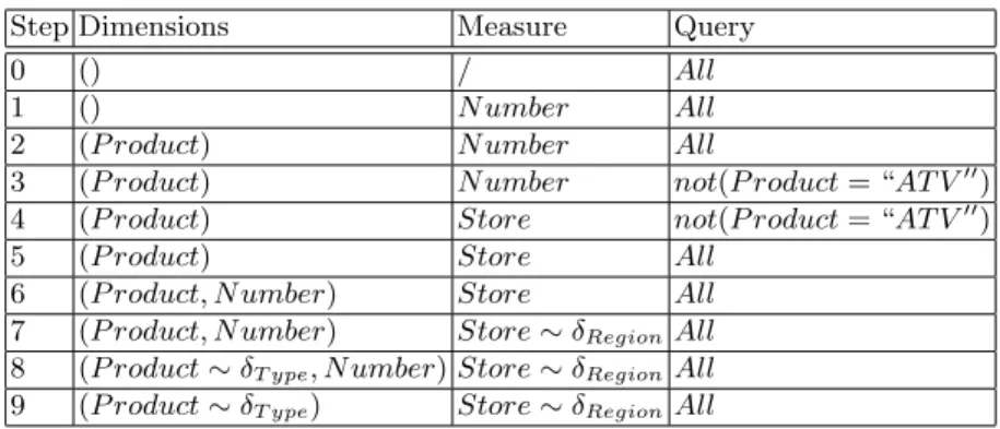
Table 5.The steps of the navigation scenario.
into a same cell, this does not change the rule at this coordinate. On the contrary, if different values are grouped into a same cell, this breaks the dependency rule at this coordinate. Figure 4 shows the two cases of value regroupments. This figure helps the user to choose navigation links, to find new rules with the help of OLAP navigation links.
5
Navigation Scenario
In this section, we present our prototype Abilis and we show its use with the ex-ample re. Abilis is a web application based on Logical Information System (LIS)
[9]. LIS allows users to query and navigate from concept to concept. LIS defines navigation links to refine the set of objects by navigating to other concepts. We have added a new view of the selected objects as a cube, as well as the OLAP navigation links.
We navigate with the example re, adding a taxonomy on each dimension.
Dates are organized by day and month; stores are organized by city and region; product are organized by article and by type. We search for dependency rules between products, numbers and stores. Table 5 presents the steps of our nav-igation scenario. Figure 5 shows our prototype at step 8. It contains (1) the current query (All means all the transactions), (2) the navigation tree (to add a dimension or refine the query) and (3) the view, displayed as a cube. Each cell of the cube shows the multiset of measure values as a tag cloud. For example, (4) shows that the support of the rule P roduct ∼ δT ype = Bike ∧ N umber =
3 → Store ∼ δRegion is 2. The size of an item in a cell depends on the support
of the rule.
The first view presents a single cell containing the 10 transactions (0). We set N umber as the measure (1). The cube has always one cell, and displays the proportion of the seven different number values (e.g. there is two sales with N umber = 4). We add a dimension P roduct (2), to check dependencies like P roduct → N umber. The resulting cube partitions the numbers into six cells,
Fig. 3.The prototype Abilis, at the step 8 of the scenario.
one per product. Each case except ATVs contains one number value. We select all transactions such that the product is not ATV (3). All cells of the resulting cube contains one number value. Therefore, there is a CFD (P roduct → N umber, Tp),
where Tp contains cells where the product is not ATV.
Now we want to work with the store locations. We change the measure to Store (4) then we select all transactions (5). The resulting cube does not contain a FD. Figure 4 shows that adding a dimension helps to have more dependencies. We then add N umber as a new dimension (6). The resulting cube has two dimen-sions and shows the CFD (P roduct, N umber → Store, Tp) with Tp containing
all the transactions except those where N umber = 3 and P roduct = BM X. In-deed, this cell contains {{Quimper, Brest}}. Those two cities being in the same region, we change the granularity level of the measure to Store ∼ δ Region (7). The resulting cube shows a FD, because each cell contains zero or one region. Figure 4 shows two possibilities of a roll-up in a dimension, with a start-ing cube containstart-ing FD: either the FD is still valid, or it is made invalid. We roll-up the P roduct dimension to P roduct ∼ δT ype (8). The FD is still valid.
Finally, we see that in each column of the current cube, there is only one re-gion. Then we delete the dimension N umber (9). The final cube shows a FD P roduct ∼ δT ype→ Store ∼ δRegion.
6
Conclusion
In this paper, we show that projecting a relation into a cube brings relevant properties. First, Association Rules, Conditional Functional Dependencies and
Functional Dependencies are made visible in this synthetic view, through the number of values in each cell. This is due to the similarity between the form premises - conclusion of the dependency rules, and the form dimensions - measure of the rules. Then, we show that the hierarchy established in [14] is consistent with our approach, and related to the number of cells containing one or zero values. Using OLAP implies that we can now see the rules at several levels of granularity.
A cube is a representation of a subset of all rules that can be extracted from a relation. We use the conventional OLAP navigation links to allow users to navigate from cube to cube, to add or to remove dimensions, or to change the granularity levels. This paper shows how to guide the user to choose navigation links. The navigation links show that some operators have a predictable behavior about the appearance or disappearance of rules.
References
1. Agrawal, R., Srikant, R.: Fast algorithms for mining association rules in large databases. In: VLDB ’94: Proceedings of the 20th International Conference on Very Large Data Bases. pp. 487–499. Morgan Kaufmann Publishers Inc., San Francisco, CA, USA (1994)
2. Bimonte, S., Tchounikine, A., Miquel, M.: Towards a spatial multidimensional model. In: DOLAP ’05: Proceedings of the 8th ACM international workshop on Data warehousing and OLAP. pp. 39–46. ACM, New York, NY, USA (2005) 3. Bra, P.D., Paredaens, J.: Conditional dependencies for horizontal decompositions.
In: Proceedings of the 10th Colloquium on Automata, Languages and Program-ming. pp. 67–82. Springer-Verlag, London, UK (1983)
4. Casali, A., Cicchetti, R., Lakhal, L.: Extracting semantics from data cubes us-ing cube transversals and closures. In: KDD ’03: Proceedus-ings of the ninth ACM SIGKDD international conference on Knowledge discovery and data mining. pp. 69–78. ACM, New York, NY, USA (2003)
5. Chakravarthy, S., Zhang, H.: Visualization of association rules over relational DBMs. In: SAC ’03: Proceedings of the 2003 ACM Symposium on Applied Com-puting. pp. 922–926. ACM, New York, NY, USA (2003)
6. Codd, E., Codd, S., Salley, C.: Provinding OLAP (On-Line Analytical Processing) to User-Analysts: An IT Mandate. Codd & Date, Inc (1993)
7. Codd, E.F.: The relational model for database management: version 2. Addison-Wesley Longman Publishing Co., Inc., Boston, MA, USA (1990)
8. Fan, W., Geerts, F., Jia, X., Kementsietsidis, A.: Conditional functional depen-dencies for capturing data inconsistencies. ACM Trans. Database Syst. 33(2), 1–48 (2008)
9. Ferr´e, S., Ridoux, O.: Logical information systems: from taxonomies to logics. In: DEXA Workshops. pp. 212–216 (2007)
10. Ganter, B., Wille, R.: Formal Concept Analysis - Mathematical Foundations (1999) 11. Han, J., Fu, Y.: Discovery of multiple-level association rules from large databases (1995), http://citeseerx.ist.psu.edu/viewdoc/summary?doi=?doi=10.1.1.39.8968 12. Huhtala, Y., K¨arkk¨ainen, J., Porkka, P., Toivonen, H.: Tane: An efficient
algorithm for discovering functional and approximate dependencies (1999), http://comjnl.oxfordjournals.org/cgi/content/short/42/2/100
13. Kivinen, J., Mannila, H.: Approximate inference of functional dependencies from relations. Theor. Comput. Sci. 149(1), 129–149 (1995)
14. Medina, R., Nourine, L.: A unified hierarchy for functional dependencies, con-ditional functional dependencies and association rules. In: ICFCA ’09: Proceed-ings of the 7th International Conference on Formal Concept Analysis. pp. 98–113. Springer-Verlag, Berlin, Heidelberg (2009)
15. Medina, R., Nourine, L.: Conditional functional dependencies: An FCA point of view. In: ICFCA. pp. 161–176 (2010)
16. Pasquier, N., Bastide, Y., Taouil, R., Lakhal, L.: Discovering frequent closed item-sets for association rules. In: ICDT ’99: Proceedings of the 7th International Con-ference on Database Theory. pp. 398–416. Springer-Verlag, London, UK (1999) 17. Shanmugasundaram, J., Fayyad, U., Bradley, P.S.: Compressed data cubes for
OLAP aggregate query approximation on continuous dimensions. In: KDD ’99: Proceedings of the fifth ACM SIGKDD international conference on Knowledge discovery and data mining. pp. 223–232. ACM, New York, NY, USA (1999) 18. Techapichetvanich, K., Datta, A.: VisAR : A new technique for visualizing mined
association rules. In: ADMA. pp. 88–95 (2005)
19. Zaki, M.J.: Generating non-redundant association rules. In: KDD ’00: Proceedings of the sixth ACM SIGKDD international conference on Knowledge discovery and data mining. pp. 34–43. ACM, New York, NY, USA (2000)