HAL Id: hal-01599438
https://hal.archives-ouvertes.fr/hal-01599438
Submitted on 17 Oct 2017
HAL is a multi-disciplinary open access
archive for the deposit and dissemination of
sci-entific research documents, whether they are
pub-lished or not. The documents may come from
teaching and research institutions in France or
abroad, or from public or private research centers.
L’archive ouverte pluridisciplinaire HAL, est
destinée au dépôt et à la diffusion de documents
scientifiques de niveau recherche, publiés ou non,
émanant des établissements d’enseignement et de
recherche français ou étrangers, des laboratoires
publics ou privés.
Optimizing concurrent configuration and planning: A
proposition to reduce computation time
Paul Pitiot, Michel Aldanondo, Élise Vareilles, T. Coudert, L. Zhang
To cite this version:
Paul Pitiot, Michel Aldanondo, Élise Vareilles, T. Coudert, L. Zhang. Optimizing concurrent
configu-ration and planning: A proposition to reduce computation time. 2013 IEEE INTERNATIONAL
CON-FERENCE ON INDUSTRIAL ENGINEERING AND ENGINEERING MANAGEMENT (IEEM
2013), 2013, Bangkok, Thailand. p. 1367-1371. �hal-01599438�
Abstract - This communication deals with mass customization and the association of the product configuration task with the planning of its production process while trying to optimize cost and cycle time. In some previous works, we have proposed an optimization algorithm, called CFB-EA. This communication concerns a way to improve CFB-EA for large problems. Previous experiments have highlighted that CFB-EA is able to find quickly a good approximation of the Pareto Front. This led us to propose to decompose the optimization in two tasks. First, a “rough” approximation of the Pareto Front is quickly searched and proposed to the user. Then the user indicates the area of the Pareto Front that he is interested in. The problem is filtered and the solution space reduced. A second optimization is launched on the focused area. Our goal is to compare the classical single task optimization with the two tasks proposed approach.
Keywords – Configuration, planning, optimization
I. INTRODUCTION
This contribution is dealing with a two steps aiding decision system that sequentially supports: (i) the interactive configuration of a product and the interactive planning and scheduling of its production process (ii) the optimization of the conflicting criteria cost and cycle time. In this context, the goal of this communication is to propose and evaluate an approach that allows reducing the optimization computation time. Section II introduces concurrent configuration and planning. Section III presents the model to optimize and the used optimization algorithm. Then it proposes the approach that reduces the computation time. Section IV describes experimental results that show the interest of the proposition. The configuration of a private aircraft illustrates the paper.
II. CONCURRENT CONFIGURATION AND PLANNING
Many authors, since [1] or [2], have defined configuration as the task of deriving the definition of a specific or customized product (through a set of properties, sub-assemblies or bill of materials, etc…) from a generic product or a product family, while taking into account specific customer requirements. Some authors, like [3] or [4] have shown that the same kind of reasoning process can be considered for production process planning. They therefore consider that deriving a specific production plan (operations, resources to be used, etc...)
from some kind of generic process plan while respecting product characteristics and customer requirements, can define production planning.
It has also been shown by many authors, as [5] and [6], that configuration and planning problems can be efficiently modelled and processed when considered as a Constraints Satisfaction Problem (CSP). CSP filtering allows interactive solution space reduction while CSP solving is open to various optimization techniques. We therefore assume that a constraint based model (product variables and constraints) of a generic product and the same kind of model for a generic production plan (process variables and constraints) can be established and we restrict the configuration and planning tasks to the instantiation of these two models. Finally in order to achieve concurrent configuration and planning, we merge the two CSPs in a single problem. This allows propagating the consequences of each decision or requirement:
- relevant to product configuration towards the planning of its production process (for example, a luxury finish requires at least two additional months),
- relevant to process planning or scheduling towards the configuration of the product (for example, such assembly duration forbids the use of such a kind of engine).
In [7] and [8], we have described how user requirements (for example, number of seats belongs to [6, 8] or due date is prior to 31/10/2010) can be processed while leaving some choices undecided (for example flying speed and range remain not set). These undecided characteristics are frequently set by commercial configuration systems with default values. Instead of using these default values, we explained that it is much better to use these undecided characteristics to optimise some criteria. In our case, we consider cost and cycle time (performance could be also considered) and propose compromise solutions on a Pareto Front. This is the basis of our two steps aiding decision system (figure 1) that allows interactive configuration and planning (all requirements are sequentially filtered) followed by a multi-criteria optimization (undecided characteristics are set).
When the problem size is small, branch and bound techniques provide Pareto Fronts in a small computation time. When the problem gets larger many authors, see [9] or [10], propose to use evolutionary algorithms to handle the problem. In this idea, we have proposed and discussed in [7] and [8] a constrained evolutionary algorithm, called CFB-EA for Constraint Filtering Based Evolutionary
Optimizing concurrent configuration and planning:
A proposition to reduce computation time
P. Pitiot
1,2, M.Aldanondo
1, E. Vareilles
1, T. Coudert
3, L. Zhang
41University Toulouse Mines Albi, France - 2 3IL-CCI Rodez, France
3 University Toulouse INP-ENIT Tarbes, France - 4 IESEG School of Management, Lille-Paris, France
Algorithm. However, for larger problem (> 1012 solutions)
Pareto computing time is quantified in days. Our goal is therefore to reduce this computing time.
Fig 1. Concurrent Configuration and planning process III. OPTIMIZING THE PROBLEM
A. Optimization problem
Given previous elements, the optimization problem can be generalized as the one shown in figure 2. The constrained optimization problem (O-CSP) is defined by the quadruplet <V, D, C, f > where V is the set of decision variables, D the set of domains linked to the variables of V, C the set of constraints on variables of V and f the multi-valuated fitness function. The set V gathers the product and process variables. The set C gathers product constraints (Cc) and process constraints (Cp). Total cost is a numerical constraint that calculates the sum of product and process cost variables. Cycle time is also a numerical constraint that calculates the sum of the process operation durations. Discrete constraints filtering is processed using a conventional arc consistency technique [11] while numerical constraints are processed using bound consistency [12].
Fig 2. Optimization problem
B. Optimization algorithm used and quality measure
Initially, EAs deal with large combinative unconstrained problems. But real-world problems are generally constrained. Many research studies try to
integrate constraints in EA. C. Coello Coello proposes a wide state of art of these methods [13]. The current tendencies in the resolution of constrained optimization problem using EAs are penalty functions, stochastic ranking, ε-constrained, multi-objective concepts, feasibility rules and special operators. CFB-EA belongs to this last family. The special operators’ class gathers methods that try to deal only with feasible individuals like repairing methods, preservation of feasibility methods or operator that move solutions within a specific region of interest within the search space.
CFB-EA is based on SPEA-2 [14] and considers only valid individuals thanks to the following modification. Each time an individual is created (initialization operator) or modified (crossover and mutation operators), every gene (decision variable of V) is randomly instantiated into its current domain. To avoid the generation of unfeasible individuals, the domain of every remaining gene is updated by constraint filtering. Thanks to consult [7] and [8] for more details.
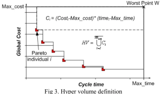
As our goal is to reduce computing time, we will have to measure performances in terms of result quality and computation time. In terms of quality, as we want to compare Pareto fronts, we use the Hypervolume measurement proposed by [15] which is illustrated in figure 3. It measures the hypervolume of the space dominated by a set of solutions. It thus allows evaluating both convergence and diversity proprieties (the fittest and most diversified set of solutions is the one that maximizes hypervolume).
Fig 3. Hyper volume definition
C. Approach for computation time reduction
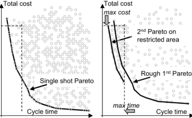
The idea proposed in this communication is to replace the Pareto front computation by two successive tasks: (i) a first rough Pareto computation that provides a global idea of possible compromises (ii) a second computation on a restricted area selected by the user. This is shown in the illustration of figure 4. The left part of figure 4 shows what we call now a “single shot Pareto”. The right part of figure 4 shows a “two-task Pareto” where a first rough Pareto is quickly obtained (first task, with less investigated solutions), followed by a zoom selected by the user (max cost and max time) and a second Pareto computation only on this restricted area (second task with a higher solution density).
Step 1 - Interactive Configuration
Planning
Step 2 Cycle time / cost
optimization Undecided choices User Requirements user
Initial solution space Solution space fine with the user Pareto optimal solutions space fine with the user
co st co st co st
Two key points of this proposition disserve to be highlighted. First, the restricted area is obtained by constraining the two criteria total cost and cycle time (or interesting area). As these two criteria are formalized as numerical constraints, they can be filtered and reduce the solution space of the whole problem. Second, the second zoom optimization task does not restart from scratch. It benefits from the individuals of the archive that belongs to the restrained area founded during first task. Next section will show how this idea reduces computation time.
Fig 4. Single shot and two-task optimization principles IV. EXPERIMENTATIONS
A. Model used
The goal of the proposed experiments is to compare these two optimization approaches: single-shot and two-task. In terms of quality we compare the two fronts with the Hypervolume. In terms of computation time, we evaluate, for a given Hypervolume result, the time reduction provided by the second approach (two-task).
In terms of problem size, we consider a model called “full_ aircraft” that gathers 92 variables (symbolic, integer or float variables) linked by 67 constraints (compatibility tables, equations or inequalities). Among these variables, we consider 21 decision variables that will be manipulated by the optimization algorithms (chromosome in EAs): 12 product variables (each with 6 possible discrete values) and 9 process variables (each with 9 possible discrete values).
Without any constraints, this provides a number of possible combinations around 1018 (≈ 612 x 99). An
average constraint level, that rejects 93% of solutions, allows 7.3*1016 feasible solutions. Results of
experimentations with other model sizes and other constraint levels can be consulted in [8].
Figure 5 shows the Pareto Fronts obtained with CFB-EA after 3 and 24 hours of computation. The rough Pareto front obtained after 3 hours of computation allows the user to decide in which area he is interested in. In the next sub-section, we will study a division of this Pareto front
in three restricted areas. These areas have been selected in order to evaluate performance of the proposed two-task approach, but it also corresponds with some classical preference of a user who could wish:
- - solutions with shortest cycle times, zoom_1: with a cycle time less than 410
- - solutions with lowest total costs, zoom_3: with a total cost less than 475
- - compromise solutions, zoom_2: cycle time less than 470 and a total cost less than 535.
Fig 5. Pareto-fronts after 3 and 24 hours of computation
B. Experimental evolutionary settings
We use classical evolutionary settings similar for both approaches: Population size: 80, Archive size: 100, Individual Mutation Probability: 0.3, Gene Mutation Probability: 0.2, Crossover Probability: 0.8.
The only other difference between single-shot CFB-EA and two-task CFB-EA is the stopping criterion. While in single-shot approach, we use a fix time limit (24 hours), the two-task approach uses a conditional stopping test that stops if there is no HV improvement after 2 hours (that are added to the three initial hours for getting the rough Pareto Front).
The goal of the following sections is to evaluate the two-task optimization on the three selected areas of the figure 5 (zoom 1, zoom 2 and zoom3) with respect to the single-shot optimization.
C. First specific result
Figure 6 shows an example of three Pareto fronts that can be obtained on the zoom 1 area:
- rough Pareto obtained after 3 hours (fig 9 squares), - two-task, after 3+12 hours (fig 9 triangles),
- single-shot, stopped after 24 hours (fig 9 diamonds). The Pareto Fronts obtained by the two approaches (single-shot and two-task) are very close when cycle is greater than 355, for lower cycle times, the proposed two-task approach is a little better. However, these curves correspond with a specific run. In order to derive stronger conclusions, 10 executions of the two approaches have been achieved for each of the three zoom areas.
Total cost
Cycle time
Single shot Pareto
Total cost Cycle time max cost max time Rough 1rstPareto 2ndPareto on restricted area
Fig 6. Example of Pareto fronts obtained on Zoom 1
D. Detailed results and comparisons
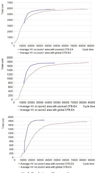
Detailed experimental results achieved on the three zoom areas are presented in figure 7 and table 1. On each graph of figure 7, the vertical axis corresponds to the hyper volume (average of ten runs) reach and horizontal one is the computer time. At time 0, the single-shot optimization is launched (dotted line). After 3 hours (10800 seconds):
- the single-shot keeps going on (dotted line),
- a zoom is performed and the two-task is launched (solid line).
The table 1 provides numeric results for each zoom area. The columns display the single-shot, two-task and % gap of:
- average final hypervolume, - average computation time,
- maximum value of hypervolume (among the 10 runs). In terms of quality or hypevolume, the new proposed approach (two-task optimization) allows obtaining a similar performance with respect to single-shot one: - 0.4% worse on zoom1, despite a higher max HV, - 1% worse on zoom2
- 4% better on zoom3
but in around half of computing time: - 13 h instead of 24h for zoom1 - 13.5h instead of 24h for zoom2 - 10.5h instead of 24h for zoom 3.
Furthermore, this computing time includes the 2 hours of computation without any hypervolume reduction before stopping (stopping criterion of the two-task approach).
It can be seen on the figure 7 that when the single-shot CFB-EA has trouble to obtain a good Pareto Front during the first three hours, the more the two-task CFB-EA is performing. On zoom1 area, single-shot CFB-EA reaches relatively quickly a near-final Pareto Front; while on zoom3 area, it reaches it very slowly.
Fig 7. Evolution of hypervolume TABLE 1 Comparison of the two approaches
Zoom 1 Single-shot CFBEA Two-task CFBEA gap in % Average Final HV 5849 5823 -0.4 Average Comp.time 86400(24h) 47996 ( 13h) -44.6 Max HV 6043 6057 0.2 Zoom 2 Average Final HV 1758 1740 -1. Average Comp.time 86400(24h) 48501 ( 13.5h) -44 Max HV 1795 1776 -1 Zoom 3 Average Final HV 1765 1844 4.4 Average Comp.time 86400(24h) 38185 ( 10.5h) -55.9 Max HV 1831 1845 0,7
IV. CONCLUSIONS
The goal of this communication was to evaluate an optimization principle that reduces the computation time of the optimization of a concurrent configuration and planning process. First the background of concurrent configuration and planning has been recalled with associated constrained modeling elements. Then the initial optimization approach (single-shot CFB-EA) was recalled followed by the description of the two-task approach object of this communication. Instead of computing a Pareto Front on the whole solution space, the key idea is: to compute quickly a rough Pareto Front, to ask the user about an interesting area, to filter the solution space on this area and to launch a second Pareto computation only on this restricted area.
According to the experimental results, the proposed two-task approach allows a significant time saving around half of the previous time needed by the single-shot optimization approach. In terms of quality, Hypervolume computations are very close or even a little better in some case. Furthermore, these results have been obtained on a rather large problem that contains around 1016/1017 solutions. With smaller problems, the proposed approach should perform much better.
These interesting results highlight two already mentioned key points of the proposition: (i) as the two criteria are formalized as numerical constraints that can be filtered, the selected area allows an efficient reduction of the solution space of the whole problem (ii) the second zoom optimization task is initialized with the results of the first one and therefore starts with a good quality archive.
Only two criteria: cycle time and cost have been used. There would be no problem to include a performance criterion as far as it can be formalized as a numerical constraint that can be filtered with bound consistency. We are already working on a more extensive test with different model sizes and different levels of constraint.
REFERENCES
[1] S. Mittal, F. Frayman, “Towards a generic model of configuration tasks” in Proc. of IJCAI 1989, pp. 1395-1401. [2] T. Soininen, J. Tiihonen, T. Männistö, and R. Sulonen, “Towards a General Ontology of Configuration.,” Artificial
Intelligence for Engineering Design, Analysis and Manufacturing, vol 12 no. 4, 1998, pp. 357–372.
[3] K. Schierholt, “Process configuration: combining the principles of product configuration and process planning,”
Artificial Intelligence for Engineering Design, Analysis and Manufacturing vol 15 no. 5, 2001, pp. 411-424.
[4] L. Zhang, E. Vareilles, M. Aldanondo, “Generic bill of functions, materials, and operations for SAP2 configuration,” Int. .Journal of Production Research, vol. 51 no. 2, 2013, pp. 465-478.
[5] U. Junker, “Configuration”, chap. 24 of the Handbook of
Constraint Programming, Elsevier, 2006, pp. 835-875.
[6] R. Barták, M. Salido, F. Rossi, “Constraint satisfaction techniques in planning and scheduling,” Journal of
Intelligent Manufacturing, vol. 21, no. 1, 2010, pp. 5-15.
[7] P. Pitiot, M. Aldanondo, E. Vareilles, P. Gaborit, M. Djefel, S. Carbonnel, “Concurrent product configuration and process planning, towards an approach combining interactivity and optimality,” Int. .Journal of Production
Research, vol. 51 no. 2, 2013 , pp. 524-541.
[8] P. Pitiot, M. Aldanondo, E. Vareilles, L. Zhang, T. Coudert, “Some Experimental Results Relevant to the Optimization of Configuration and Planning Problems,” Lecture Notes in
Computer Science Volume 7661, 2012, pp 301-310.
[9] G. Hong, D. Xue, Y. Tu, “Rapid identification of the optimal product configuration and its parameters based on customer-centric product modeling for one-of-a-kind production,” Computers in Industry, vol.61 no. 3, 2010, pp. 270–279.
[10] L. Li, L. Chen, Z. Huang, Y. Zhong, “Product configuration optimization using a multiobjective GA,” Int..Journal of
Advance Manufacturing Technology, vol. 30, 2006, pp.
20-29.
[11] C. Bessiere, “Constraint propagation,” chap. 3 of the
Handbook of Constraint Programming, Elsevier, 2006, pp.
29-70.
[12] O. Lhomme, “Consistency techniques for numerical CSPs,”
in proc. of IJCAI 1993, pp. 232-238.
[13] E. Mezura-Montes, C. Coello Coello, “Constraint-Handling in Nature-Inspired Numerical Optimization: Past, Present and Future,” Swarm and Evolutionary Computation, vol. 1 no. 4, 2011, pp. 173-194
[14] E. Zitzler, M. Laumanns, L. Thiele, “SPEA2: Improving the Strength Pareto Evolutionary Algorithm,” in Technical
Report 103, Swiss Fed. Inst. of Technology, Zurich, 2001.
[15] E. Zitzler, L. Thiele, “Multiobjective optimization using evolutionary algorithms - a comparative case study,” proc. of
5th Int. Conf. on parallel problem solving from nature, Eds.