Visual question answering with modules and language modeling

Université de Montréal

Visual Question Answering with Modules and Language

Modeling

par

Vardaan Pahuja

Département d’ informatique et de recherche opérationnelle Faculté des arts et des sciences

Mémoire présenté à la Faculté des études supérieures et postdoctorales en vue de l’obtention du grade de

Maître ès sciences (M.Sc.) en Informatique

avril 2019

Université de Montréal

Département d' informatique et de recherche opérationnelle, Faculté des arts et des sciences

Ce mémoire intitulé

Visual Question Answering with Modules and Language Modeling

Présenté par

Vardaan Pahuja

A été évalué par un jury composé des personnes suivantes Alain Tapp Président-rapporteur Christopher J. Pal Directeur de recherche Yoshua Bengio Membre du jury

Résumé

L’objectif principal de cette thèse est d’apprendre les représentations modulaires pour la tâche de réponse visuelle aux questions (VQA). Apprendre de telles représentations a le potentiel de généraliser au raisonnement d’ordre supérieur qui prévaut chez l’être humain. Le chapitre 1 traite de la littérature relative à VQA, aux réseaux modulaires et à l’optimisation de la structure neuro-nale. En particulier, les différents ensembles de données proposés pour étudier cette tâche y sont détaillés. Les modèles de VQA peuvent être classés en deux catégories en fonction des jeux de données auxquels ils conviennent. La première porte sur les questions ouvertes sur les images na-turelles. Ces questions concernent principalement quelques objets/personnes présents dans l’image et n’exigent aucune capacité de raisonnement significative pour y répondre. La deuxième catégorie comprend des questions (principalement sur des images synthétiques) qui testent la capacité des modèles à effectuer un raisonnement compositionnel. Nous discutons de différentes variantes ar-chitecturales de réseaux de modules neuronaux (NMN). Finalement nous discutons des approches pour apprendre les structures ou modules de réseau neuronal pour des tâches autres que VQA.

Au chapitre 2, nous décrivons un moyen d’exécuter de manière parcimonieuse un modèle CNN (ResNeXt [110]) et d’enregistrer les calculs effectués dans le processus. Ici, nous avons utilisé un mélange de formulations d’experts pour n’exécuter que les K meilleurs experts dans chaque bloc convolutionnel. Le groupe d’experts le plus important est sélectionné sur la base d’un contrôleur qui utilise un système d’attention guidé par une question suivie de couches entièrement connec-tées dans le but d’attribuer des poids à l’ensemble d’experts. Nos expériences montrent qu’il est possible de réaliser des économies énormes sur le nombre de FLOP avec un impact minimal sur la performance.

Le chapitre 3 est un prologue du chapitre 4. Il mentionne les contributions clés et fournit une introduction au problème de recherche que nous essayons de traiter dans l’article. Le chapitre 4 contient le contenu de l’article. Ici, nous nous intéressons à l’apprentissage de la structure interne

des modules pour les réseaux de modules neuronaux (NMN) [3, 37]. Nous introduisons une nou-velle forme de structure de module qui utilise des opérations arithmétiques élémentaires et la tâche consiste maintenant à connaître les poids de ces opérations pour former la structure de module. Nous plaçons le problème dans une technique d’optimisation à deux niveaux, dans laquelle le modèle prend des gradients de descente alternés dans l’architecture et des espaces de poids. Le chapitre 5 traite d’autres expériences et études d’ablation réalisées dans le contexte de l’article précédent.

La plupart des travaux dans la littérature utilisent un réseau de neurones récurrent tel que LSTM [33] ou GRU [13] pour modéliser les caractéristiques de la question. Cependant, les LSTM peuvent échouer à encoder correctement les caractéristiques syntaxiques de la question qui pourraient être essentielles [87]. Récemment, [76] a montré l’utilité de la modélisation du langage pour répondre aux questions. Avec cette motivation, nous essayons d’apprendre un meilleur modèle linguistique qui peut être formé de manière non supervisée. Dans le chapitre 6, nous décrivons un réseau ré-cursif de modélisation de langage dont la structure est alignée pour le langage naturel. Plus tech-niquement, nous utilisons un modèle d’analyse non supervisée (Parsing Reading Predict Network ou PPRN [86]) et augmentons son étape de prédiction avec un modèle TreeLSTM [99] qui utilise l’arborescence intermédiaire fournie par le modèle PRPN dans le but de un état caché en utilisant la structure arborescente. L’étape de prédiction du modèle PRPN utilise l’état caché, qui est une combinaison pondérée de l’état caché du TreeLSTM et de celui obtenu à partir d’une attention structurée. De cette façon, le modèle peut effectuer une analyse non supervisée et capturer les dépendances à long terme, car la structure existe maintenant explicitement dans le modèle. Nos expériences démontrent que ce modèle conduit à une amélioration de la tâche de modélisation du langage par rapport au référentiel PRPN sur le jeu de données Penn Treebank.

Mots clés : Réponse visuelle à une question, raisonnement visuel, réseaux modulaires, optimi-sation de la structure neuronale, modélioptimi-sation du langage

Summary

The primary focus in this thesis is to learn modularized representations for the task of Visual Question Answering. Learning such representations holds the potential to generalize to higher order reasoning as is prevalent in human beings. Chapter 1 discusses the literature related to VQA, modular networks and neural structure optimization. In particular, it first details different datasets proposed to study this task. The models for VQA can be categorized into two categories based on the datasets they are suitable for. The first one is open-ended questions about natural images. These questions are mostly about a few objects/persons present in the image and don’t require any significant reasoning capability to answer them. The second category comprises of questions (mostly on synthetic images) which tests the ability of models to perform compositional reasoning. We discuss the different architectural variants of Neural Module Networks (NMN). Finally, we discuss approaches to learn the neural network structures or modules for tasks other than VQA.

In Chapter 2, we discuss a way to sparsely execute a CNN model (ResNeXt [110]) and save computations in the process. Here, we used a mixture of experts formulation to execute only the top-K experts in each convolutional block. The most important set of experts are selected based on a gate controller which uses a question-guided attention map followed by fully-connected layers to assign weights to the set of experts. Our experiments show that it is possible to get huge savings in the FLOP count with only a minimal degradation in performance.

Chapter 3 is a prologue to Chapter 4. It mentions the key contributions and provides an in-troduction to the research problem which we try to address in the article. Chapter 4 contains the contents of the article. Here, we are interested in learning the internal structure of the modules for Neural Module Networks (NMN) [3, 37]. We introduce a novel form of module structure which uses elementary arithmetic operations and now the task is to learn the weights of these operations to form the module structure. We cast the problem into a bi-level optimization technique in which the model takes alternating gradient descent steps in architecture and weight spaces. Chapter 5

discusses additional experiments and ablation studies that were done in the context of the previous article.

Most works in the literature use a recurrent neural network like LSTM [33] or GRU [13] to model the question features. However, LSTMs can fail to properly encode syntactic features of the question which could be vital to answering some VQA questions [87]. Recently, [76] has shown the utility of language modeling for question-answering. With this motivation, we try to learn a better language model which can be trained in an unsupervised manner. In Chapter 6, we discuss a recursive network for language modeling whose structure aligns with the natural language. More technically, we make use of an unsupervised parsing model (Parsing Reading Predict Network or PPRN [86]) and augment its prediction step with a TreeLSTM [99] model which makes use of the intermediate tree structure given by PRPN model to output a hidden state by utilizing the tree structure. The predict step of PRPN model makes use of a hidden state which is a weighted combination of the TreeLSTM’s hidden state and the one obtained from structured attention. This way it helps the model to do unsupervised parsing and also capture long-term dependencies as the structure now explicitly exists in the model. Our experiments demonstrate that this model leads to improvement on language modeling task over the PRPN baseline on Penn Treebank dataset.

Keywords: Visual Question Answering, Visual Reasoning, Modular Networks, Neural Struc-ture Optimization, Language Modeling

Contents

Résumé . . . iii

Summary . . . v

List of Tables . . . xi

List of Figures . . . xiii

List of Abbreviations . . . xv

Acknowledgments . . . xvii

Introduction. . . 1

Chapter 1. Background . . . 3

1.1. Visual Question Answering . . . 3

1.2. VQA Datasets. . . 3

1.2.1. Natural Image datasets . . . 3

1.2.2. Synthetic image datasets . . . 5

1.3. Evaluation metrics . . . 6

1.4. Neural Architectures for VQA . . . 6

1.4.1. Attention-based Neural Architectures . . . 6

1.4.1.1. Models for Open-ended questions . . . 6

1.4.1.2. Models for compositional reasoning based questions . . . 8

1.4.2. Modular Neural Architectures. . . 11

1.6. Modular Networks for other tasks . . . 14

Chapter 2. Learning Sparse Mixture of Experts for Visual Question Answering . . . 15

2.1. Introduction. . . 15

2.2. Related Work . . . 15

2.3. Model Architecture . . . 17

2.3.1. Bottleneck convolutional block. . . 18

2.3.2. Gate controller . . . 21

2.4. Experiments . . . 22

2.4.1. VQA v2 dataset . . . 22

2.4.2. CLEVR dataset . . . 22

2.5. Conclusion . . . 23

Chapter 3. Prologue to First Article. . . 25

3.1. Article details . . . 25

3.2. Context . . . 25

3.3. Contributions . . . 26

Chapter 4. Learning Neural Modules for Visual Question Answering . . . 27

4.1. Introduction. . . 27

4.2. Background . . . 28

4.2.1. Module Layout Controller . . . 29

4.2.2. Operation of Memory Stack for storing attention maps . . . 29

4.2.3. Final Classifier . . . 30

4.3. Learnable Neural Module Networks . . . 30

4.3.1. Structure of the Generic Module . . . 30

4.3.1.2. Generic Module with 4 inputs . . . 33

4.3.2. Overall structure . . . 33

4.4. Experiments . . . 34

4.4.1. Results . . . 36

4.4.2. Measuring the role of individual arithmetic operators . . . 38

4.4.3. Measuring the sensitivity of modules . . . 38

4.4.4. Visualization of module network parameters. . . 39

4.5. Related Work . . . 39

4.6. Conclusion . . . 41

Bibliography for First Article (Chapter 4) . . . 42

Appendix for First Article (Chapter 4) . . . 45

4.A. Answer Module schematic diagrams . . . 46

4.B. Hand-crafted modules of Stack-NMN . . . 47

4.C. Visualization of module structure parameters. . . 48

Chapter 5. Additional Experiments for Learning Neural Modules for Visual Question Answering . . . 51

5.1. Experiments for a different variant of model structure . . . 51

5.2. Experiments for sparsity at node level . . . 51

5.3. Results . . . 54

Chapter 6. Learning a recursive network whose structure aligns with natural language 57 6.1. Introduction and Related Work . . . 57

6.2. Overview of PRPN model . . . 58

6.4. Experiments . . . 61

6.5. Conclusion . . . 63

General Conclusion. . . 65

Bibliography . . . 67 Appendix A. Figures showing realization of basic modules using v2 of cell structure . . . A-i

List of Tables

1.1 Implementation details of neural modules (adapted from [37]) . . . 13

2.1 Modular CNN for VQA v2 model. . . 19

2.2 Modular CNN for Relational Networks Model . . . 19

2.3 Results on VQA v2 validation set . . . 23

2.4 Results on CLEVR v1.0 validation set (Overall accuracy) . . . 23

4.1 Number of modules of each type for different model ablations.. . . 34

4.2 CLEVR and CLEVR-Humans Accuracy by baseline methods and our models. (*) denotes use of extra supervision through program labels. (‡_{) denotes training from raw} pixels. † _{Accuracy figures for our implementation of Stack-NMN. The original paper} reports 93% validation accuracy, test accuracy isn’t reported. . . 35

4.3 Model Ablations for LNMN (CLEVR Validation set performance). The term ‘map_dim’ refers to the dimension of feature representation obtained at the input or output of each node of cell. . . 36

4.4 Analysis of gradient attributions of ↵ parameters corresponding to each module (LNMN (9 modules)), summed across all examples of CLEVR validation set. . . 37

4.5 Analysis of performance drop with removing operators from a trained model (LNMN 9 modules) on CLEVR validation set. . . 37

4.6 Analytical expression of modules learned by LNMN (11 modules). In the above equations,Pdenotes sum over spatial dimensions of the feature tensor. . . 40

4.B.1 Neural modules used in [36]. The modules take image attention maps as inputs, and output either a new image attention aout or a score vector y over all possible answers

( is elementwise multiplication;Pis sum over spatial dimensions). . . 48 5.1 CLEVR Accuracy (val. set) for different versions of LNMN models . . . 55 5.2 CLEVR Accuracy (val. set) for different versions of LNMN models for node sparsity . 56 6.1 Perplexity on the Penn Treebank test set . . . 62

List of Figures

1.1 Architecture diagram for Multimodal Compact Bilinear (MCB) with Attention (adapted

from [23]). . . 7

1.2 Relational Networks model architecture (adapted from [82]) . . . 9

1.3 Schematic representation of FiLM based model architecture for Visual Reasoning (adapted from [75]). . . 10

2.1 Model architecture for VQA v2 dataset (adapted from [102]) . . . 18

2.2 Model architecture for Relational Networks (adapted from [82]) . . . 18

2.3 Architecture of a sample block of ResNeXt-101 (32 ⇥ 4d). . . 19

2.4 Architecture of corresponding block of conditional gated ResNeXt-101 (32 ⇥ 4d) assuming we choose to turn ON paths with top k gating weights. Here i1,· · · ,ik denote the indices of groups in top k. . . 20

4.1 Attention Module schematic diagram (3 inputs). . . 32

4.2 Attention Module schematic diagram (4 inputs). . . 32

4.3 Visualization of module structure parameters (LNMN (11 modules)). For each module, each row denotes the ↵0 = (↵)parameters of the corresponding node. . . 41

4..4 Q1: What number of cylinders are gray objects or tiny brown matte objects? A: 1 Q2: Is the number of brown cylinders in front of the brown matte cylinder less than the number of brown rubber cylinders? A: no . . . 46

4..5 Plot of variation of w with epochs. . . 46

4.A.1 Answer Module schematic diagram (3 inputs) . . . 47

4.C.1 Visualization of module structure parameters (LNMN (9 modules)). For each module, each row denotes the ↵0

= (↵)parameters of the corresponding node. . . 49 4.C.2 Visualization of module structure parameters (LNMN (14 modules)). For each module,

each row denotes the ↵0

= (↵)parameters of the corresponding node. . . 50 5.1 Attention Module schematic diagram version 2 (3 inputs). . . 52 5.2 Attention Module schematic diagram version 2 (4 inputs). . . 52 5.1 Comparison of variation of mean entropy of ↵0

. . . 56 6.1 Training curve for PRPN + TreeLSTM model . . . 63 A.1 Schematic diagram for realization of Find Module. . . A-i A.2 Schematic diagram for realization of Compare Module. . . A-ii A.3 Schematic diagram for realization of Filter Module. . . A-ii A.4 Schematic diagram for realization of And Module.. . . .A-iii A.5 Schematic diagram for realization of Or Module. . . .A-iii A.6 Schematic diagram for realization of Scene Module. . . .A-iv A.7 Schematic diagram for realization of Transform Module. . . .A-iv A.8 Schematic diagram for realization of Answer Module. . . A-v

List of Abbreviations

VQA Visual Question Answering

MS-COCO Microsoft Common Objects in Context MLP Multi Layer Perceptron

ReLU Rectified Linear Unit

CNN Convolutional Neural Network LSTM Long Short-Term Memory

GRU Gated Recurrent Unit FLOP Floating Point Operation

conv. convolutional

NMN Neural Module Network

GAN Generative Adversarial Network MCB Multimodal Compact Bilinear

BoW Bag of Words

RGBD Red Green Blue Depth

NLVR Natural Language for Visual Reasoning PRPN Parsing-Reading-Predict Network

Acknowledgments

I am immensely grateful to a lot of people who have helped me in my research. The most fruitful part during this journey was played by my advisor Prof. Christopher Pal. Under his able supervision, I got familiar with the research methodology for machine learning. He helped me strengthen my basics. His precise insights about potential issues with training machine learning models were crucial to making them work. I acknowledge the support of the Natural Sciences and Engineering Research Council of Canada (NSERC) under the COHESA network for research funding. I thank my collaborators Jie Fu and Sarath Chander for their contribution in the article titled “Learning Neural Modules for Visual Question Answering”. I also thank Zhouhan Lin for mentoring me in the language modeling aspect. I acknowledge the help of Massimo Caccia in translating the summary to French. I thank Evan Racah and Harm de Vries for helpful discussions. I am thankful to Compute Canada and Calcul Québec for providing me the computational resources for running my experiments. I also acknowledge the support of Nvidia for NVIDIA NGC Deep Learning Containers and the DGX-1 gifted to our lab. Finally, I wish to thank my family especially my mother for her support and encouragement during the course of my research.

Introduction

Visual Question Answering is one of the most interesting tasks in machine learning. It involves the twin challenges of understanding the two modalities involved i.e. language and vision, plus understanding one in the context of the other. Human intelligence is remarkably proficient in capturing the relationship between different objects in a scene and and being able to process this information to answer questions in conversations. However, most neural-network based models of this task have been susceptible to learning biases in datasets than perform actual reasoning [115] and are thus prone to adversarial attacks. A plausible way to increase human trust in deploying such models for practical applications is to make their decision making process explainable to users. One way to achieve this would be to decompose the model into sub-modules which are designed for specific functions. In Chapter 4, we address the task of learning the internal structure of modules for VQA models for answering compositional reasoning based questions. In Chapter 2, we try to learn a modularized version of ResNeXt CNN [110] model for the task of VQA. The key contribution of this work is to efficiently train VQA models by sparsely executing the CNN sub-network. Visual Question Answering models can benefit from language modeling for obtaining a syntax-aware feature representation for the question and also for generating variable length answer tokens. To this end, we propose a language model which can be trained in an unsupervised manner and also capture long-term dependencies in Chapter 6.

Chapter 1

Background

1.1. Visual Question Answering

Visual Question Answering (VQA) has received considerable attention in the machine learning community in recent years. This can be attributed to the fact that it is seen as an AI-complete problem i.e. if given an image, a system is capable of answering any reasonable question, then any vision task could be trivially broken into a set of questions about the subject image.

1.2. VQA Datasets

1.2.1. Natural Image datasets

TheDAQUAR [63] is one of the first datasets which addresses VQA as its core learning task. It is built on top of the NYU-Depth V2 dataset [71] which contains RGBD images of indoor scenes. The questions comprise of both synthetic ones (generated automatically based on some templates and then instantiated with facts from database) and the ones which are crowd-sourced from human workers. It contains 6794 training and 5674 test question-answer pairs in total. The answer-set contains 894 object categories, colors, numbers or sets of those. The main drawback of this dataset is that the answers to the questions are biased towards certain objects like table or chair.

TheCOCO-QA [79] contains questions generated on the images of MS-COCO image dataset [57]. The questions are generated synthetically by converting the image descriptions to questions. It contains 78736 training and 38948 test question-answer pairs. The authors discarded the answers which appear too frequently or too rarely resulting in a more balanced answer distribution.

Visual Genome [54] is one of the largest VQA datasets by size with over 1.77 million ques-tion answer pairs. There are to sub-categories of quesques-tions - freeform QAs (which are based on

the entire image) and region-based QAs (based on selected regions of the image). This dataset contains annotations for a large number of objects in images, scene graphs and region descriptions in addition to question-answer pairs. It uses the images present in the intersection of YFCC100M [103] and MS-COCO [57] datasets.

VQA-real [4] This is the most widely used VQA dataset for questions on natural images. The images correspond to 123,287 training and validation images and 81,434 test images from the Microsoft Common Objects in Context (MS COCO) dataset. The questions are crowd-sourced from human annotators. It contains 614,163 questions and 10 answers per question from unique workers. Each question can thus possibly have multiple correct answers. The main shortcoming of this dataset is that given a question type, the answer distribution is highly skewed in certain cases. For instance, the answer for 39% of counting questions is ‘2’ and ‘tennis’ is the answer for questions like “What sport is” in 41% of the cases [26]. In order to alleviate such biases present in the dataset, a second version of the dataset was proposed (called VQA v2 [26]). In this dataset, the authors try to balance the questions by asking human annotators to create a new question (I0

,Q,A0) for an (image, question, answer) triplet (I,Q,A) such that I 6= I0

and A 6= A0

, but I is similar to I0. In this way, I and I0 are very close in visual feature space, so it is tough for the model to give both answers correctly without properly understanding the visual modalities.

NLVR2 _{[92] This is a dataset based on web photographs in which each example consists of a}

caption paired with two photographs. The task is to predict whether the caption is True or False. This task requires complex reasoning which includes comparative, quantitative and spatial reason-ing on the objects present in the images. This is similar to spirit to CLEVR [48] but the images are natural images instead of synthetic ones and the captions are crowd-sourced from human anno-tators. This dataset poses twin challenges of complex visual reasoning and understanding human specified captions. It contains a total of 107,292 examples.

GQA [41] is a recently proposed dataset for visual reasoning and compositional question an-swering on real-world images. It uses the images in Visual Genome dataset [54] that have scene graph annotations to create a semantic ontology over the scene graph vocabulary. The questions are created from 524 templates/patterns using the content present in scene graphs. It contains 22.6M questions over 113K images. All the questions have their respective functional programs included in the dataset. This dataset is strategically designed to mitigate the flaws of previous datasets which

lead models to exploit different kinds of biases rather than perform actual reasoning to achieve good accuracy.

1.2.2. Synthetic image datasets

SHAPES [3] is a dataset of synthetic images which emphasizes the understanding of spatial and logical relations among multiple objects. It contains 244 unique questions, pairing each ques-tion with 64 different images, resulting in a total of 15616 unique quesques-tion-answer pairs.

TheCLEVR [48] dataset proposed on similar lines as SHAPES, contains questions that test visual reasoning abilities such as counting, comparison, logical reasoning based on 3D shapes like cubes, spheres and cylinders of varied shades. Though it is in similar spirit to SHAPES, the CLEVR dataset is much more complex than SHAPES both in terms of complexity and variety of questions and images. Notably the number of questions in CLEVR dataset is around 1 million (compared to 15K in SHAPES), which has contributed it to became a standard benchmark for a variety of visual reasoning models.

VQA abstract scenes In order to make VQA systems focus on the task of visual reasoning rather than recognition, a new dataset named VQA abstract scenes was proposed in [4] along with the main natural image version. It contains scenes of paperdoll models in a variety of indoor and outdoor scenes. The complexity of this dataset is enhanced by models of different ages, gender and races, with different face expressions and pose variations. It contains a total of 50K scenes and 150K questions. [26] introduces a complementary abstract scenes dataset such that in a given example, the two scenes have opposite answers to the same boolean question. The motivation for this dataset is to prevent the model from exploiting language biases for performance but instead focus on visual reasoning.

NLVR The Cornell Natural Language Visual Reasoning (NLVR) [93] is a dataset aimed at test-ing the ability of VQA systems to answer compositional questions ustest-ing a visual context. Unlike CLEVR [48] and SHAPES [3] which use synthetic questions, here the questions are crowd-sourced from human annotators. The question is a description of the image and there are two images asso-ciated with it. The description is true for only one of the given images and the task of the model is to guess the correct image for the given description. It contains 3,962 unique descriptions and 92,244 examples.

1.3. Evaluation metrics

Some VQA models like [64] output natural language answers to questions. For such models, the evaluation is difficult as it amounts to paraphrase detection, which is itself a topic of active research. [63] proposes the use of Wu-Palmer Set (WUPS) score. This is inspired from Fuzzy Sets literature as many objects in the set of answers tend to be similar (e.g. ‘cup’ and ‘mug’), so all incorrect (as per ground truth) answers should not be penalized equally. Here, W UP (a, b) [109] represents the similarity between two words a and b based on their depth in the taxonomy tree. The VQA-real dataset [4] contains answers from 10 human annotators for each question. A predicted answer is deemed 100 % correct if 3 or more annotators gave that answer.

accuracy = min✓no. of annotators who gave that answer

3 , 1

◆

[41] introduces some new evaluation metrics like consistency, validity, plausibility and grounding for measuring the coherent reasoning capabilities of VQA models.

1.4. Neural Architectures for VQA

The span of attention-based neural architectures can be broadly classified into two categories, mainly based on the datasets they are suitable for. The first category of architectures is designed pri-marily for questions based on real images which are mostly crow-sourced from human annotators. In such cases, the questions can be open-ended and mostly concern objects present in the image, but the compositional reasoning ability required to answer questions present in such datasets, is fairly limited. COCO-QA [79], DAQUAR [63], Visual Genome [54] and VQA-real [4] are some examples in the first category. The second category of model architectures is primarily designed for datasets containing questions which test the compositional reasoning ability of models and are mostly synthetically generated. This category includes datasets like SHAPES [3], CLEVR [48] and NLVR [93].

1.4.1.1. Models for Open-ended questions

CNN + BoW [118] is a very naive baseline model for VQA in which the question representa-tion is obtained as a Bag of Words [81] of embeddings of individual quesrepresenta-tion words. The visual features are obtained from GoogLeNet [95].

CNN + LSTM In this baseline model [63], the image features are encoded using a CNN like VGGNet [88], ResNet [31] etc. The final hidden state of LSTM [33] which takes the question word embeddings as input, is used for question representation. Both the image and question rep-resentations are concatenated and then passed through an MLP to get the distribution over the set of answers. [79] proposes an approach to handle answers of different word lengths in which an encoder LSTM takes the concatenation of image and question feature vectors as input. A de-coder LSTM decodes the ende-coder representation to produce a variable sized string of words for the answer until a special token indicating the end of sentence is predicted.

Multimodal Compact Bilinear Pooling (MCB) [23] In this model, the question and image features are obtained from LSTM and CNN respectively like previous models. It uses Multi-modal Compact Bilinear pooling (MCB) [24] to fuse the two Multi-modalities instead of concatenation or element-wise sum or product. This fusion takes place at each location of the spatial grid of features obtained from the CNN. Subsequently, two convolutional layers followed by softmax are used to predict the soft attention score for each location. The weighted sum of visual features using the attention map is again fused with the question representation using MCB. The features thus obtained are passed through an MLP followed by softmax to get the distribution over the set of answers. Figure 1.1 illustrates the VQA architecture which uses MCB.

What is the color of the vehicle? C N N (R e sN e t1 5 2 ) W E , L S T M T ile Multimodal Compact Binlinear C o n v, R e L U C o n v S o ftm a x W e ig h te d S u m Multimodal Compact Binlinear S o ftm a x F C Red 2048 x 14 x 14 2048 x 14 x 14 16k x 14 x 14 2048 2048 16k 30 0 0 2048

Figure 1.1. Architecture diagram for Multimodal Compact Bilinear (MCB) with Attention (adapted from [23]).

Stacked Attention Networks (SAN) [111] In this model, the model first generates an attention over the image pixels by fusing the spatial image features vI and question features vQ.

hA = tanh(WI,AvI (WQ,AvQ+ bA))

pI =softmax(WPhA+ bP)

where vI 2 Rd⇥m, vQ 2 Rd, WI,A, WQ,A 2 Rr⇥d, bA 2 Rr , WP 2 R1⇥r and bP 2 Rm.

pI _{2 R}m _{corresponds to the attention probability assigned to m image regions. Here, d denotes}

the feature dimension of each image region in the final conv. layer and r is a hyper-parameter for the size of a parameter matrix. denotes a matrix-vector summation operation. The weighted sum of visual features using the attention map (denoted by ˜vI) is added to the question feature vector

vQto form the query vector u.

˜ vI = X i pI ivi u =˜vI + vQ

The attention process described above is repeated for K attention layers. The updated query vector uk_{denotes the more fine-grained query in the multimodal space after the k}th _{attention step.}

hk_A = tanh(W_I,Ak vI (WQ,Ak uk 1+ bkA))

pI,k =softmax(W_Pkhk_A+ bk_P) ˜ v_Ik =X i pI,k_i vi uk _=˜vk I + uk 1

The final query vector uK is fed to the classifier to predict the distribution over the set of answers.

1.4.1.2. Models for compositional reasoning based questions

Relational Networks [82] This model incorporates the explicit use of relational features be-tween every pair of objects to predict the answer distribution.

vIQ =

X

i,j

g([vi, vj, q])

Here, q denotes the question representation, vi and vj denote the spatial features (obtained from

CNN) corresponding to the ith_{and j}th_{image regions and g denotes an MLP. The feature}

represen-tation vIQ is passed through a classifier to get the answer distribution. A schematic diagram for

What number of cylinders are gray objects or tiny brown matte

objects?

*

What number of ...objects

+ (answer)1

Final CNN feature maps

Conv. object LSTM Object pair with question Element-wise sum RN Image: question:

Figure 1.2. Relational Networks model architecture (adapted from [82])

Feature-wise Linear Modulation (FiLM) [75] uses Conditional Batch Normalization [17, 19] (CBN) conditioned on the question features to modulate the visual features for predicting the answer. More specifically, FiLM learns the parameters of Batch Normalization of each channel as affine functions of the GRU [15] representation of the question.

i,c = fc(xi) i,c = hc(xi)

F iLM (Fi,c| i,c, i,c) = i,cFi,c+ i,c

Here, xi denotes the ith input example’s question representation and ( i,c, i,c) denotes the BN

parameters for the ith_{input and c}th_{channel. The model architecture consists of a CNN (either}

pre-trained or pre-trained from scratch) followed by four residual blocks. Each residual block consists of a 1⇥1 convolution layer followed by a 3⇥3 convolution layer and a batch-normalization layer whose ( , )parameters are controlled by FiLM. The classifier (comprising of a 2-layer MLP followed by softmax) uses the features output by FiLM network to output a distribution over the answers. A schematic representation of different components of the FiLM model is shown in Figure 1.3.

Memory, Attention, and Composition (MAC) Network [40] The MAC network consists of an input unit, a recurrent unit comprising of a number of MAC cells stacked together and an output unit. A MAC cell consists of a control unit, read unit and write unit.

The input unit ingests the two modalities i.e. the question and image and converts them into their respective distributed feature representations. For the question, a word-embedding is trained from scratch and the features are obtained using a Bidirectional LSTM [33]. The model makes

GRU GRU GRU GRU GRU GRU GRU What number cylinders of objects gray are Linear Resblock 1 Resblock 2 Resblock N CNN Classifier Conv ReLU Conv ReLU BN FiLM

+

Figure 1.3. Schematic representation of FiLM based model architecture for Visual Reasoning (adapted from [75]).

use of the LSTM outputs at each time-step of the question. For the image, a ResNet101 [32] (pre-trained on ImageNet [18]) is used to extract conv-4 spatial features from the image.

The function of the control unit is to perform an attention on question words and subsequently guide the reasoning operation. Let [cw1, cw2, ..., cwS] denote the output of Bi-LSTM at each

time-stamp of the input sequence of question words. Let q denote the concatenation of final hidden state of Bi-LSTM during the forward and backward passes. qidenotes the question’s transformed

representation for the ith _{reasoning step. At first, q}

i and ci 1 are concatenated and combined

through a linear transform to form cqi. Then, cai,sis computed as the similarity coefficient of cqi

with the Bi-LSTM feature representation of question words. Finally, ci represents the weighted

feature representation of Bi-LSTM outputs obtained using these similarity values.

qi = Wid⇥2dq + bdi

cqi = Wd⇥2d[ci 1,qi] + bd

cai,s = W1⇥d(cqi cws) + b1

cvi,s =softmax(cai,s)

ci = S

X

s=1

The image features represent the knowledge base KH⇥W ⇥d _{= {k}d h,w|

H,W

h,w=1,1} where d is the

number of output channels of the CNN. H and W denote the height and width of the visual feature maps respectively. In the above equations, the superscript with the parameter tensors denotes their dimension. The function of the read unit is to retrieve the information required for the ith_reasoning

step. The function of the write unit is to compute the result of ith_{reasoning step and store it in the}

memory state mi.

1.4.2. Modular Neural Architectures

Neural Module Networks [2] is a technique for answering complex questions which involve spatial, set-theoretic reasoning and the ability to recognize attributes of shapes and objects. Each “module” is a neural network whose structure is pre-specified in terms of layers and whose param-eters are learnt during training. The universal dependency parse representation is obtained using Stanford Parser [53]. Next, the set of dependencies is converted into structured queries each of which consists of a function and a short word phrase which the function operates on. These func-tions are then mapped to modules based on the location in the parse tree, of the node they operate on. Thus, a custom layout of modules is obtained for each question. This model obtains excellent results on SHAPES dataset (introduced in this paper only). The main contribution of this model is that it uses the syntax tree efficiently to generalize well to complex questions involving compo-sitional reasoning. The drawback is that the layout predictor is heavily hand-engineered for this particular dataset and it has to be re-specified for use on other datasets.

End-to-End Module Networks for Visual Question Answering (N2NMN) [37] This model builds upon the approach of Neural Module Networks (NMNs) but improves it in many ways. The layout predictor is not hand-engineered but a policy network with a sequence-to-sequence RNN which outputs a sequence of tokens (denoted by m(t) _{) corresponding to the Reverse Polish}

notation [10] of the syntax tree of modules. The input question (of T words) is encoded using an encoder LSTM to obtain a set of encoder states [h1, h2,· · · , hT]. The decoder is an Attentional

to each word of the input sequence: uti = vT tanh(W1hi+ W2h 0 t) ↵ti = exp(uti) PT j=1exp(utj) ct= T X i=1 ↵tihi Here, h0

t denotes the hidden state of decoder LSTM at timestep t, ct denotes the context vector

and q denotes the question representation. v, W1 and W2 are learnable parameter tensors. The

probability of the next token of the layout sequence is predicted as:

p(m(t)_|m(1),_{· · · , m}(t 1), q) = softmax(W3ht+ W4ct)

The probability of a particular layout l in the space of layouts can be written as

p(l|q) = Y m(t)_2l p(m(t)|m(1)_{,· · · , m}(t 1)_{, q)} xtxt = T X i=1 ↵tihi

The policy samples a high probability layout according to the probability p(l|q) and a network of modules is thus assembled. At test time, the maximum probability layout is selected using beam-search. The neural modules take 0, 1 or 2 attention maps as input along with visual features xvisand

textual features xtxt. The implementation details of these modules are shown in Table 1.1. The xvis

is obtained from the conv-4 layer of ResNet-101 (similar to MAC network). The textual feature for module m is computed as the weighted combination of embedding vectors of the question words, weighted by attention vector ↵ti computed by the decoder LSTM. Since the layout sampling is

non-differentiable, it is trained using a combination of backpropagation and policy gradient. Stack-NMN Stack-NMN [36] is an end-to-end differentiable version of Neural Module Net-works. It eliminates the major limitation of previous approaches in this direction [2, 37] that hand engineer the layout or learn it by policy gradient. It uses soft program execution to train the entire model and gradually makes the layout hard towards the end of training by adding an entropy loss term. Please refer to Section 4.2 for more details on this model.

Transparency by Design network [65] builds upon the End-to-End Module Networks [37] but makes an important change in that the proposed modules explicitly utilize attention maps passed

Module name Att-inputs Features Output Implementation details

find (none) xvis, xtxt att aout= conv2(conv1(xvis) W xtxt)

relocate a xvis, xtxt att aout= conv2(conv1(xvis) W1sum(a xvis) W2xtxt)

and a1, a2 (none) att aout= minimum(a1, a2)

or a1, a2 (none) att aout= maximum(a1, a2)

filter a xvis, xtxt att aout= and(a, find[xvis, xtxt]())

[exist,

count] a (none) ans y = W

T_vec(a)

describe a xvis, xtxt ans y = W1T(W2sum(a xvis) W3xtxt)

[eq_count,

more, less] a1, a2 (none) ans y = W

T

1vec(a1) + W2Tvec(a2)

compare a1, a2 xvis, xtxt ans y = W1T(W2sum(a1 xvis) W3sum(a2 xvis) W4xtxt)

Table 1.1. Implementation details of neural modules (adapted from [37])

as inputs instead of learning whether or not to use them. This results in more interpretability of the modules since they perform specific functions. It improves the state of art on the CLEVR CoGenT dataset. [48].

Neural Compositional Denotational Semantics for Question Answering [29] constructs a parse-chart over the entire space of parse trees by using a parser similar to CRF-based PCFG parser which uses the CYK algorithm [30, 49, 113]. Each node in the parse chart represents a span of the question. Each token in the question can be an entity, relation, ungrounded semantic type, a truth value or a semantically vacuous word. The composition modules transform the input semantic types into output tokens. It reports good accuracy on CLEVRGEN, a new dataset over CLEVR images which specifically tests semantic operators like conjunction, negation, count etc.

ReasonNet [42] uses two types of modules: visual classification modules and visual attention modules, similar to [37]. The modules are hand-engineered to output specific visual features e.g. object detection, object classification, scene classification, face detection etc. It uses a bilinear model [100] to pool the module’s representation and the question representation.

1.5. Neural Structure Optimization

Neural Architecture Search (NAS) is a technique to automatically learn the structure and con-nectivity of neural networks rather than training human-designed architectures. In [120], a recur-rent neural network (RNN) based controller is used to predict the hyper-parameters of a CNN such as number of filters, stride, kernel size etc. They used REINFORCE [108] to train the controller

with validation set accuracy as the reward signal. Among other approaches that use reinforcement learning to perform architecture search, [121] uses proximal policy optimization (PPO) [83] in-stead of REINFORCE. In [117], Q-learning [106] is used to construct network blocks which are then stacked together to form the complete network. As an alternative to reinforcement learn-ing, evolutionary algorithms [91] have been used to perform architecture search in [77, 68, 60, 78]. Recently, [59] proposed a differentiable approach to perform architecture search and reported success in discovering high-performance architectures for both image classification and language modeling.

1.6. Modular Networks for other tasks

[52] proposes an EM style algorithm to learn black-box modules and their layout for image recognition and language modeling tasks. [1] proposes an approach called modular meta-learning to learn modules (parameterized as MLPs) and a compositional scheme to compose these modules in order to re-use them for new tasks. Progressive Module Networks [50] is a model for multi-task learning for a variety of visual reasoning multi-tasks such as image captioning, counting and visual question answering. It builds modules which are compositional i.e. utilize lower-level modules to produce their output. [116] makes use of modules for training Generative Adversarial Networks (GANs) [25]. The main advantage of this is that modules can be re-used and composed to form GANs for generating images in a specific domain at test time.

Chapter 2

Learning Sparse Mixture of Experts for Visual Question

Answering

2.1. Introduction

Deep learning has enabled commendable progress in many machine learning tasks. The ability to train bigger networks (in terms of parameters) with improved infrastructure has enhanced the performance in several tasks like object recognition, object detection, machine translation, face recognition, question-answering etc. However, this poses a serious challenge in terms of huge computational resources that are required to train and deploy such huge models. We aim to tackle this issue for the specific task of Visual Question Answering (VQA). A Convolutional Neural Network (CNN) is an integral part of the visual processing pipeline of a VQA model (assuming the CNN is trained along with entire VQA model). In this project, we propose an efficient and modular neural architecture for the VQA task with focus on the CNN module. Our experiments demonstrate that a sparsely activated CNN based VQA model achieves comparable performance to a standard CNN based VQA model architecture.

2.2. Related Work

Mixture of Experts Mixture of Experts [45] is a formulation in machine learning which em-ploys the divide-and-conquer principle to solve a complex problem by dividing the neural network into several expert networks. In the Mixture of MLP Experts (MME) method [105, 72, 21], a gat-ing network is used to assign a weight gi to the output of the corresponding expert network. The

final output of the ensemble is a weighted sum of outputs of each of the individual expert networks. O = N X i=1 oigi

Here, there are are total of N experts and oidenotes the output of the ithexpert. The gating network

is an MLP followed by softmax operator. [47] uses a mixture of experts for visual reasoning tasks in which each expert is a stack of residual blocks.

Conditional Computation Conditional Computation is the technique of activating only a sub-portion of the neural network depending on the inputs. For instance, if a visual question answering system has to count the number of a specified object vs if it has to tell the color of an object, the specific features needed to give the correct answer in either case are different. Hence, there is a potential to reduce the amount of computation the network has to perform in each case, which can be especially useful to train large deep networks efficiently. The use of stochastic neurons with bi-nary outputs to selectively turn-off experts in a neural network has been explored in [8]. [16] uses a low-rank approximation of weight matrix of MLP to compute the sign of pre-nonlinearity activa-tions. In case of ReLU activation function, it is then used to optimize the matrix multiplication for the MLP layer. [7] uses Policy gradient to sparsely activate units in feed-forward neural networks by relying on conditional computation. [85] proposes Sparsely-Gated Mixture-of-Experts layer (MoE) which uses conditional computation to train huge capacity models on low computational budget for language modeling and machine translation tasks. It makes use of noisy top-K mech-anism in which a random noise is added to gating weights and then top-K weights are selected. Another line of work makes use of conditional computation in VQA setting. DPPNet [73] makes use of a dynamic parameter layer (fully-connected) conditioned on the question representation for VQA. ABC-CNN [11] predicts convolutional kernel weights using an MLP which takes question representation as input. Here, the advantage is that the question conditioned convolutional kernels can filter out unrelated image regions in the visual processing pipeline itself.

Computationally efficient CNNs [39] proposes Multi-Scale Dense Convolutional Networks (MSDNet) to address two key issues in (i) budgeted classification- distribute the computation bud-get unevenly across easy and hard examples, (ii) anytime prediction: the network can output the prediction result at any layer depending on the computation budget without significant loss in ac-curacy. The optimization of computational complexity of CNNs at inference-time has been studied in [9] in which an adaptive early-exit strategy is learned to by-pass some of the network’s layers in

order to save computations. MobileNet [34] uses depth-wise separable convolutions to build light weight CNNs for deployment on mobile devices.

CNN architectures The invention of Convolutional Neural Networks (CNNs) has led to a re-markable improvement in performance for many computer vision tasks [55, 61, 80]. In recent years, there has been a spate of different CNN architectures with changes to depth [89], topology [32, 96], etc. The use of split-transform-merge strategy for designing convolutional blocks (which can be stacked to form the complete network) has shown promise for achieving top performance with a lesser computational complexity [96, 97, 98, 110]. The ResNeXt [110] CNN model pro-poses cardinality (size of set of transformations in a convolutional block) as another dimension apart from depth and width to investigate, for improving the performance of convolutional neural networks. Squeeze-and-Excitation Networks [35] proposes channel-wise attention in a convolu-tional block and helped improve the state of art in ILSVRC 2017 classification competition.

Grouped Convolution In grouped convolution, each filter convolves only with the input fea-ture maps in its group. The use of grouped convolutions was first done in AlexNet [55] for training a large network on 2 GPUs. A recently proposed CNN architecture named CondenseNet [38] makes use of learned grouped convolutions to minimise superfluous feature-reuse and achieve computational efficiency.

2.3. Model Architecture

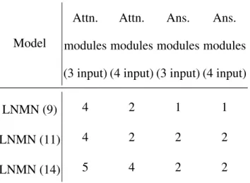
Our main goal is to optimize the convolutions performed by the Convolutional Neural Network (CNN) in a conditional computation setting. We use an off-the-shelf neural architecture for both VQA v2 [26] and CLEVR [48] datasets and just replace the CNN with a modularized version of the ResNeXt [110] CNN as we describe below. The details of convolutional architecture used in the VQA v2 model and CLEVR model are illustrated in Table 2.1 and Table 2.2 respectively. For VQA v2, we used the model architecture proposed in [102]. A schematic diagram to illustrate the working of this model is given in Figure 2.1. For CLEVR dataset, we use the Relational Networks [82] model because it is one of the few models which is fully-supervised and trains the CNN in the main model pipeline. A diagram to illustrate the working of this model is shown in Figure 2.2.

Word embedding CNN GRU L2 norm softmax W Question Image W W W W W W W + 14 14 x 300 N K 2048 512 512 300 N N 512 K x 2048 512

Top-down attention weights

Concatenation

Weighted sum over image locations

Element-wise product

1.0

0.0

Soft ground truth scores

Predicted scores of candidate answers

Cross-entropy loss

Figure 2.1. Model architecture for VQA v2 dataset (adapted from [102])

What number of cylinders are gray objects or tiny brown matte

objects?

*

What number of ...objects

+ (answer)1

Final CNN feature maps

Conv. object LSTM Object pair with question Element-wise sum RN Image: question:

Figure 2.2. Model architecture for Relational Networks (adapted from [82])

2.3.1. Bottleneck convolutional block

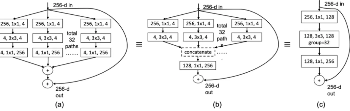
The architecture of a residual block of ResNeXt-101 (32 ⇥ 4d) is shown in Figure 2.3. Using algebraic manipulations, it can be shown that Figure 2.3(a), (b) and (c) are equivalent in terms of the function computed by it. Using grouped convolution (with number of groups=32), Figure 2.3(c) is an optimum way of implementing it in standard libraries. We introduce a gating mechanism to assign weights to each of the paths (which equal 32 in the example shown). We treat each path as a convolutional module which should potentially be used for a specific function. The gate values are normalized to sum to unity and are conditioned on the LSTM based feature representation of the question. The working of gate controller is detailed in section 2.3.2.

In order to optimize the computation of a ResNeXt residual block, we execute just the top-k (out of 32) paths and zero out the contribution of others. This is based on the hypothesis that the gate controller shall determine the most important modules (aka paths) to execute by assigning higher weights to more important modules. Figure 2.4 (a-d) shows the transformation of modular-ized ResNeXt-101 (32⇥4d) block to its grouped convolution form. This technique is similarly ap-plicable for the convolutional block used for CLEVR dataset (shown in Table 2.2). In our efficient

Figure 2.3. Architecture of a sample block of ResNeXt-101 (32 ⇥ 4d)

stage output Description

conv1 112⇥112 7⇥7, 64, stride 2

conv2 56⇥56

3⇥3 max pool, stride 2 2 6 6 6 6 6 4 1⇥1, 128 3⇥3, 128, C=32 1⇥1, 256 3 7 7 7 7 7 5 ⇥3 conv3 28⇥28 2 6 6 6 6 6 4 1⇥1, 256 3⇥3, 256, C=32 1⇥1, 512 3 7 7 7 7 7 5 ⇥4 conv4 14⇥14 2 6 6 6 6 6 4 1⇥1, 512 3⇥3, 512, C=32 1⇥1, 1024 3 7 7 7 7 7 5 ⇥23 conv5 7⇥7 2 6 6 6 6 6 4 1⇥1, 1024 3⇥3, 1024, C=32 1⇥1, 2048 3 7 7 7 7 7 5 ⇥3

Table 2.1. Modular CNN for VQA v2 model

stage output Description

conv1 64⇥64 3⇥3, 64, stride 2

conv2 32⇥32

3⇥3 max pool, stride 2 2 6 6 6 6 6 4 1⇥1, 48 3⇥3, 48, C=12 1⇥1, 48 3 7 7 7 7 7 5 ⇥1 conv3 16⇥16 2 6 6 6 6 6 4 1⇥1, 48 3⇥3, 48, C=12 1⇥1, 48 3 7 7 7 7 7 5 ⇥1 conv4 8⇥8 2 6 6 6 6 6 4 1⇥1, 48 3⇥3, 48, C=12 1⇥1, 48 3 7 7 7 7 7 5 ⇥1 conv5 8⇥8 1_{⇥ 1 conv. layer}

with 24 o/p channels

Table 2.2. Modular CNN for Relational Networks Model

implementation, we avoid executing the groups which don’t fall in top-k. More technically, we ag-gregate the non-contiguous groups of the input feature map, which fall in top-k, into a new feature

Figure 2.4. Architecture of corresponding block of conditional gated ResNeXt-101 (32 ⇥ 4d) assuming we choose to turn ON paths with top k gating weights. Here i1,· · · ,ik denote the

indices of groups in top k.

map. We perform the same trick for the corresponding convolutional and batch-norm weights and biases.

Computational complexity of the ResNeXt convolutional block (in terms of floating point operations)⇤₌

⇤. No. of FLOPS of a convolutional block (no grouping) = Cin⇤ Cout⇤ p ⇤ p ⇤ Ho⇤ Wo, No. of FLOPS of a

convolutional block (with grouped convolution) = Cin⇤Cout⇤p⇤p⇤Ho⇤Wo

k where Cin, Cout, p, k, Ho, Wo denote the

number of input channels, no. of output channels, kernel size, no. of groups, output feature map height and width respectively

=complexity(conv-reduce) + complexity(conv-conv)+

complexity(conv-expand) + complexity(bn-reduce, bn, bn-expand) =feature-dim ⇤ (k ⇤ d) ⇤ 1 ⇤ 1 ⇤ H_o1⇤ W1 o + (k⇤ d) ⇤ (k ⇤ d) ⇤ 3 ⇤ 3 k ⇤ H 2 o ⇤ Wo2 + (k_{⇤ d) ⇤ feature-dim ⇤ 1 ⇤ 1 ⇤ Ho}3_{⇤ Wo}3+ O(k) = k_{⇤ d ⇤ feature-dim ⇤ Ho}1_{⇤ Wo}1+ k_{⇤ d ⇤ feature-dim ⇤ Ho}3_{⇤ Wo}3 + 9⇤ d2_{⇤ k ⇤ H}2 o ⇤ Wo2+ O(k)

Notation: conv-reduce, conv-conv and conv-expand denote the 1⇥1, 3⇥3 and 1⇥1 convolutional layers in a ResNeXt convolutional block (in that order).

Here, d denotes the size of group in group convolution (equals 4 for Figure 2.4) and ‘feature dim’ denotes the no. of channels in the feature map input to the convolutional block. The imple-mentation of modularized ResNeXt block is more efficient than the regular impleimple-mentation in the case when k < 32. The overhead of the gate controller can be minimized by appropriate selection of hyper-parameters. The comparison of FLOPS with varying values of the hyper-parameter k is shown in Table 2.3 for the VQA v2 model and Table 2.4 for the CLEVR model.

2.3.2. Gate controller

The gate controller takes as input the LSTM based representation of the question and the inter-mediate convolutional map which is the output of the previous block. Given the image features vI

and question features vQ, we perform the fusion of these features, followed by a linear layer and

softmax to generate the attention pI _{over the pixels of the image feature input.}

˜ vI = X i pIivi uquery = ˜vI + vQ g = Wguquery+ bg g0 = ReLU (g) ||ReLU(g)||1

Notation: WI 2 RA⇥B, WI,A 2 RC⇥B, WQ,A 2 RB⇥C, WP 2 R1⇥C, bP 2 R1⇥D,

Wg 2 RB⇥E, bg 2 RB⇥1, A = Feature dim. of each img. region in final conv. layer, B =

E = No. of modules/residual blocks. We add an additional loss term which equals the square of coefficient of variation (CV) of gate values for each convolutional block.

CV (g0) = ( PN i=1g 0 i,·) µ(PN_i=1g_i,0_·) In the above equation, g0

i,· 2 RE denotes the gating weight vector for the ithbatch example. This

helps to balance out the variation in gate values [85] otherwise the weights corresponding to the modules which get activated initially will increase in magnitude and this behavior reinforces itself as the training progresses.

2.4. Experiments

We use the Bottom-up attention model for VQA v2 dataset as proposed in [101] as our base model and replace the CNN sub-network with our custom CNN. The corresponding results are shown in Table 2.3. The results show that there is a very minimal loss in accuracy from 0% sparsity to 50% sparsity. However, with 75% sparsity†_{, there is a marked 3.62% loss in overall}

accuracy.

2.4.2. CLEVR dataset

We use the Relational Networks model [82] and replace the Vanilla CNN used in their model with our modularized CNN and report the results on the CLEVR v1 dataset. The CNN used for this model has four layers with one residual ResNeXt block each followed by a 1⇥1 convolutional layer. The results for these experiments are shown in Table 2.4. The results show that with a slight dip in performance, the model which uses 50% sparsity has comparable performance with the one which doesn’t have sparsity in the convolutional ResNeXt block.

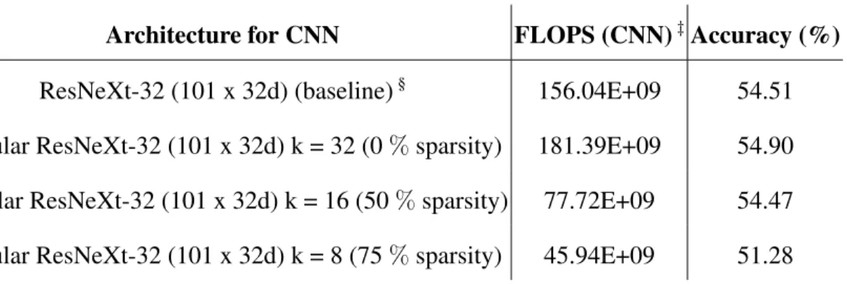
†. Here, 75% sparsity means that 75% of the modules/paths in the ResNeXt convolutional block are turned off. ‡. The FLOPS calculation assumes an input image of size 224 ⇥ 224 ⇥ 3

§. The baseline model doesn’t use R-CNN based features, so the accuracy is not directly comparable with state of the art approaches.

Architecture for CNN FLOPS (CNN)‡_{Accuracy (%)}

ResNeXt-32 (101 x 32d) (baseline)§ _{156.04E+09 54.51}

Modular ResNeXt-32 (101 x 32d) k = 32 (0 % sparsity) 181.39E+09 54.90 Modular ResNeXt-32 (101 x 32d) k = 16 (50 % sparsity) 77.72E+09 54.47 Modular ResNeXt-32 (101 x 32d) k = 8 (75 % sparsity) 45.94E+09 51.28

Table 2.3. Results on VQA v2 validation set

CNN Model description FLOPS (CNN)¶_{Val. Acc. (%)}

Modular CNN, k=12 (baseline) 5.37E+07 94.05 Modular CNN, k=6, 50 % sparsity 3.21E+07 92.23 Table 2.4. Results on CLEVR v1.0 validation set (Overall accuracy)

2.5. Conclusion

We presented a general framework for utilizing conditional computation to sparsely execute a subset of modules in a convolutional block of ResNeXt model. The amount of sparsity is a user-controlled hyper-parameter which can be used to turn off the less important modules conditioned on the question representation, thereby increasing the computational efficiency. Future work may include studying the utility of this technique in other multimodal machine learning applications which support use of conditional computation.

Chapter 3

Prologue to First Article

3.1. Article details

Learning Neural Modules for Visual Question Answering by Vardaan Pahuja, Jie Fu, Sarath Chandar, Christopher Pal was submitted to Association for Computational Linguistics (ACL) 2019 conference and is currently under review.

Personal Contribution: The initial idea for the alternating optimization of module structure and module parameters was jointly proposed by Vardaan Pahuja and Jie Fu. I was responsible for coming up with the generalized module structure and the idea of using elementary arithmetic operations to form the module operations. The idea of using Integrated Gradients [94] for mea-suring module sensitivity and other post-analysis techniques were suggested by me. The initial draft of the paper was written by me. I was also responsible for the entire code implementation in PyTorch [74] library and running different experiments related to training, post-analysis and hyper-parameter optimization.

Contribution of other authors: Jie Fu and Prof. Christopher Pal helped in initial brainstorm-ing about the project and model structure in particular. Sarath Chander helped to accelerate the progress by giving insights on appropriate selection of hyper-parameters. He also suggested the idea of adding a sparsity loss to get a sparse set of module weights at each node in module. Finally, everyone contributed to improving the draft of the paper.

3.2. Context

In this paper, we are interested in the task of Visual Reasoning, which is an important compo-nent of Visual Question Answering. Section 1.4.1.2 discusses monolithic black-box architectures

for visual reasoning like FiLM [75], Relational Networks [82] and MAC Network [40]. The sec-ond class of architectures [3, 37] (mentioned in Section 1.4.2) consist of modules which are neural networks (trained from scratch) specialized to perform a particular function.

3.3. Contributions

A major limitation of the modular neural architectures discussed in the previous section is that the modules being used were hand-engineered. In this work, we try to learn the structure of mod-ules in terms of elementary arithmetic operations. Our results show that we achieve comparable performance as the model with hand-designed modules. We present a detailed analysis of the degree to which each module influences the prediction function of the model, the effect of each arithmetic operation on overall accuracy and the analytical expressions of the learned modules.

Chapter 4

Learning Neural Modules for Visual Question Answering

Abstract

Visual question answering involves both visual recognition and reasoning grounded in language. Broadly speaking, there are two popular neural approaches to this problem domain. One family of ap-proaches tends to be based on more black-box architectures that perform the fusion of vision and language through multiple steps of attention. Another family of approaches involves human-specified neural modules, each specialized in a specific form of reasoning, where the order of execution of the underlying modules is sometimes learned. In this work, we further expand the second approach and learn the underlying internal structure of modules in terms of simple and elementary arithmetic operators. Our results show that one is indeed able to simultaneously learn both internal module structure and module sequencing, without extra su-pervisory signals for module execution sequencing. With this approach, we report performance comparable to the models using hand-designed modules.

4.1. Introduction

Visual question answering requires a learning model to answer sophisticated queries about visual inputs. Such reasoning is considered the hallmark of human intelligence and allows us to interpret and draw plausible inferences from our daily interaction with objects present in the environment. Significant progress has been made in this direction to design neural networks which can answer queries about images. However, recent studies [10, 11] have shown that the neural networks tend to exploit biases in the datasets without learning how to actually reason.

There are two broad classes of approaches proposed in the literature for the task of visual reasoning. The first class of approaches propose end-to-end black-box architectures. Examples include FiLM [18] and MAC [8] where the fusion of representations of the two modalities (image and text) is performed by using a variety of neural network architectures. The second class of

approaches are modular networks where each module is designed to focus on a sub-component of the reasoning process.

[2] propose Neural Module Network (NMN) where they compose neural network modules (with shared parameters) for each input question based on the layout predicted by the syntactic parse of the question. The modules take as input the images or the attention maps and return attention maps or labels as output. In [7], the layout prediction is relaxed by learning a layout policy with a sequence-to-sequence RNN. This layout policy is jointly trained along with the parameters of the modules. The model proposed in [6] avoids the use of reinforcement learning to train the layout predictor, and uses soft program execution to jointly learn both layout and module parameters.

A fundamental limitation of these previous modular approaches to visual reasoning is that the modules need to be hand-specified. This might not be feasible when one has limited knowledge of the kinds of questions or associated visual reasoning required to solve the task. In this work, we present an approach to learn the module structure, along with the parameters of the modules in an end-to-end differentiable training setting. Our proposed model, Learnable Neural Module Network (LNMN), learns the structure of the module, the parameters of the module, and the way to compose the modules based on just the regular task loss. Our results show that we are able to learn the structure of the modules automatically and still perform comparable to hand-specified modules. We would like to highlight the fact that our goal in this paper is not to beat the performance of the hand-specified modules since they are specifically engineered for the task. Instead, our goal is to explore the possibility of designing general purpose reasoning modules in a completely data-driven fashion.

4.2. Background

In this section, we describe the working of the Stack-NMN model [6] as our proposed LNMN model uses this as the base model. The Stack-NMN model is an end-to-end differentiable model for the task of Visual Question Answering and Referential Expression Grounding [21]. It addresses a major drawback of prior visual reasoning models in literature that compositional reasoning is im-plemented without need of supervisory signals for composing the layout at training time. It consists of several hand-specified modules (namely Find, Transform, And, Or, Filter, Scene, Answer, Com-pare and NoOp) which are parameterized, differentiable, and implement common routines needed

in visual reasoning and learns to compose them without strong supervision. The implementation detail of these modules is given in Appendix (see Table 4.B.1). The different sub-components of the Stack-NMN model are described below.

4.2.1. Module Layout Controller

The structure of the controller is similar to the one proposed in [8]. The controller first encodes the question using a bi-directional LSTM [5]. Let [h1, h2, ..., hS]denote the output of Bi-LSTM

at each time-step of the input sequence of question words. Let q denote the concatenation of final hidden state of Bi-LSTM during the forward and backward passes. q can be considered as the encoding of the entire question. The controller executes the modules iteratively for T times. At each time-step, the updated query representation u is obtained as:

u = W2[W1(t)q + b1; ct 1] + b2

where W(t)

1 2 Rd⇥d, W2 2 Rd⇥2d, b1 2 Rd, b2 2 Rd. ct 1 is the textual parameter from the

previous time step. The controller has two outputs viz. the textual parameter at step t (denoted by ct) and the attention on each module (denoted by vector w(t)). The controller first predicts an

attention on each of the words of the question and then uses this attention to do a weighted average over the outputs of the Bi-LSTM.

cvt,s= sof tmax(W3(u hs)) ct = S X s=1 cvt,s· hs

where, W3 2 R1⇥d. The attention on each module w(t)is obtained by feeding the query

represen-tation at each time-step to a Multi-layer Perceptron (MLP).

w(t)= sof tmax(M LP (u; ✓M LP))

4.2.2. Operation of Memory Stack for storing attention maps

In order to answer a visual reasoning question, the model needs to execute modules in a tree-structured layout. In order to facilitate this sort of compositional behavior, a differentiable memory pool to store and retrieve intermediate attention maps is used. The memory stack (with length denoted by L) stores H ⇥ W dimensional attention maps, where H and W are the height and width of image feature maps respectively. Depending on the number of attention maps required as

input by the module, it pops them from the stack and later pushes the result back to the stack. The model performs soft module execution by executing all modules at each time-step. The updated stack and stack pointer at each subsequent time-step are obtained by a weighted average of those corresponding to each module using the weights w(t) _{predicted by the module controller. This is}

illustrated by the equations below:

(A(t)_m, p(t)_m) =run-module(m, A(t), p(t)) A(t+1) = X m2M A(t)_{m · wm}(t) p(t+1) = sof tmax(X m2M p(t)_{m · wm}(t)) Here, A(t)

m and p(t)m denote the stack and stack pointer respectively, after executing module m at

time-step t. A(t) _{and p}(t) _{denote the stack and stack pointer obtained after the weighted average}

of those corresponding to all modules at previous time-step (t 1). The working of module layout controller and its interfacing with memory stack is illustrated in Algorithm 1. The internal functioning of a module is shown in Appendix (see Algorithm 3).

4.2.3. Final Classifier

At each time-step of module execution, the weighted average of output of the Answer modules is called memory features (denoted by f(t)

mem = P_{m2ans. module}o(t)mw(t)m). Here, o(t)m denotes the

output of module m at time t. The memory features are given as one of the inputs to the Answer modules at the next time-step. The memory features at the final time-step are concatenated with the question representation, and then fed to an MLP to obtain the logits.

4.3. Learnable Neural Module Networks

In this section, we introduce Learnable Neural Module Networks (LNMNs) for visual reason-ing, which extends Stack-NMN. However, the modules in LNMN are not hand-specified. Rather, they are generic modules as specified below.

4.3.1. Structure of the Generic Module

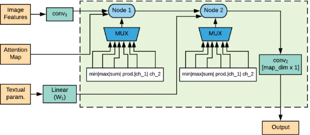
The cell (see Figures 4.1, 4.2) denotes a generic module which can span all the required mod-ules for a visual reasoning task. Each cell contains a certain number of nodes. The function of a node (denoted by O) is to perform a weighted sum of outputs of different arithmetic operations