Visualization and prediction of spatial deformation using thin-plate splines in the context of scoliosis

3/oy

z

Université de Montréal

Visualization and prediction

0f

spatial

deformation using thin-plate spiines in the

context of scoliosis

par Di Jiarig

Département d’informatique et de recherche opérationnelle facilité des arts et des sciences

Mémoire présenté à la faculté des études supérieures en vue de l’obtention du grade de

Maître ès sciences (M.Sc.) en informatique

Août 2003

) (4

)

__ C _ \/,

_Q)L9

n

Université

(1h

de Montréal

Direction des bibliothèques

AVIS

L’auteur a autorisé l’Université de Montréal à reproduire et diffuser, en totalité ou en partie, par quelque moyen que ce soit et sur quelque support que ce soit, et exclusivement à des fins non lucratives d’enseignement et de recherche, des copies de ce mémoire ou de cette thèse.

L’auteur et les coauteurs le cas échéant conservent la propriété du droit d’auteur et des droits moraux qui protègent ce document. Ni la thèse ou le mémoire, ni des extraits substantiels de ce document, ne doivent être imprimés ou autrement reproduits sans l’autorisation de l’auteur.

Afin de se conformer à la Loi canadienne sur la protection des

renseignements personnels, quelques formulaires secondaires, coordonnées ou signatures intégrées au texte ont pu être enlevés de ce document. Bien que cela ait pu affecter la pagination, il n’y a aucun contenu manquant.

NOTICE

The author of this thesis or dissertation has granted a nonexclusive license allowing Université de Montréal to reproduce and publish the document, in part or in whole, and in any format, solely for noncommercial educational and research purposes.

The author and co-authors if applicable retain copyright ownership and moral

rights in this document. Neither the whole thesis or dissertation, nor

substantial extracts from it, may be printed or otherwise reproduced without the author’s permission.

In compliance with the Canadian Privacy Act some supporting forms, contact information or signatures may have been removed from the document. While this may affect the document page count, it does not represent any loss of content from the document.

Université de Montréal Faculté des études supérieures

Ce mémoire de maîtrise intitulé

Visualization and prediction

0f

spatial deformation using

thin-plate splines in the context

0f

scoliosis

présenté par Di Jiang

a été évalué par un jury composé des personnes suivantes

Max Mignotte président-rapporteur Neil F. $tewart directeur de recherche Farida Chenet membre du jury

Sommaire

La scoliose est une déformation tridimensionnelle de la colonne vertébrale qui engendre des déformations du torse. Le risque d’un cancer associé à la méthode de diagnostique actuelle, les rayons X, appelle aux changements dans ce domai;e. Ceci est particulièrement important considérant le grand nombre de ca.s chez les adolescents. L’ordinateur a pris un rôle de plus en plus important dans le domaine

médical, au point (l’avoir été utilisé pour presque toutes les différentes parties du corps humain.

Plusieurs techniques de déformation spatiale ont été développées: les déformations sans contraintes (free-for’rn) et leurs multiples extensions, les modèles de lissage par splines, la technique “space deformation”, etc. Elles offrent à l’usager un contrôle sur la déformation par divers moyens: points marqueurs, treillis de contrôle et mampulations directes.

Dans ce projet, pour résoudre le problème de visualisation et de simulation de la scoliose, une méthode de déformation spatiale, les plaques minces (thin plate sptine modets) a été employée. Pour la prédiction de la scoliose, nous tra vaillons à la fois sur un ensemble d’indexes de R’, utilisé pour l’interpolation et l’approximation spatiale, et un ensemble d’indexes de l’intervalle [0,1] pour l’interpolation et l’extrapolation dans le temps. Nous testons et validons nos modèles avec des données de vrais patients. Les résultats des tests sur les données réelles que nous avons obtenus sont raisonnables, en se basant sur le niveau de précision des données disponibles: les résllltats de déformation externe sont plutôt bons, tant dis que les résultats de déformation interne montrent quelques erreurs. Des travaux ultérieurs pourraient se concentrer sur ces deux points, augmenter

SOMMAIRE y

la précision des données réelles et prendre en compte pius d’information interne physique.

Une contribution particulière de ce projet est que nous montrons le lieu entre les plaques minces sur un ensemble d’indexes de l’intervalle [0,1] et un ensemble d’indexes de R’. Il s’agit de deux modèles differents de spiines, mais après tout le travail mathématique (permutation et comparaison), nous pouvons voir qu’ils partagent vraiment quelque chose en commun, ce qui est très utile.

Mots clefs:

simulation médical, visualisation, modèls de plaques minces, modélisation d’objets déformarbles, scoliose.

Abstract

Scoliosis is a common 3D spinal deformity that leads to aesthetic deformity of the torso. The cancer risk associated with the current diagnosis method, X-rays, motivates modifications of this method. This is especially important because of the high occurrence of scoliosis among teenagers. The computer lias begun to ta.ke more and more important roles in the medical field; it has been used to study almost every part of the human body.

Many spatial deformation techniques have been developed: Free-form deforma tion and its several extensions, smoothing spiine models, space deformations,etc. They offer the user control over deformation hy different means: marker points, control lattices and even direct manipulations.

This project approached the problem of visualization and prediction of scoliosis with a method of spatial deformation, specifically, thin-plate spiine models. For the prediction of scoliosis, we work on both the R” index set, which we use for spatial interpolation and approximation, and the time index set, which we use for time-interpolation and time-extrapolation. We test and validate our models with real patient data. The real testing resuits we got are reasonable, based on the accuracy level of the available data: the external deformation resuits are pretty good, whule the internai deformation resuits show some errors. Later work could extend from these two points, increase the accuracy of the reaÏ data and take more internai physical information into account.

A special contribution of this project is: we show the link between the thin plate spiine modeis based on [0,1] index set and R” index set. These are two different spline models, but after some mathematical work (permutation and com

ABSTRACT _vii

parison), we cari see that they really share something in common, which is quite useful.

Keywords:

medical simulation, visualization, thin-plate spiine models, modeling ofdeformable objects, scoliosis.

Contents

Sommaire iv Abstract vi Acknowledgment xv 1 Introduction 1 1.1 Background 1 1.1.1 Scoliosis 1 1.1.2 Motivations 3

1.2 Available deformation techniques 5

1.2.1 Spatial deformation . . . 5

1.2.2 Physics-based deformation 6

1.3 Outiine of the thesis 6

2 Spatial deformatiori 8

2.1 Thin-plate spiine model $

2.2 Free-form deformation and its extensions 9

2.2.1 Theoretical foundation 9

2.2.2 FFD in our application 10

2.2.3 Preliminary experimental results using FFD 13

2.2.4 Extended versions of fFD model 15

2.3 Direct-manipulation deformation 17

CONTENTS ix

3 Smoothing Spiine Models 18

3.1 Note on terrninology 19

3.1.1 Interpolation and tirne-interpolation 19

3.1.2 Recapitulation 19

3.2 The case T = [0, 1] 20

3.2.1 Mathernatical outiine 20

3.2.2 Permuting variables for later comparison 24

3.2.3 Time-illterpolation 25

3.2.4 Time-extrapolation 27

3.3 The case T 28

3.3.1 Mathematical outiine 28

3.3.2 Anisotropic marker points 32

3.4 Comparison between [0,1] index inodel and Rd index moclel . . . 35

3.4.1 Sirnilarities 35

3.4.2 Differences 36

4 Models for simulation of deformation 38

4.1 Affine-affine matching 38

4.2 Other prediction models 40

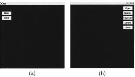
5 System interface 44

5.1 The data 44

5.2 The operations 45

5.3 The interface 46

6 Experimental Results 51

6.1 Test case analysis 51

6.1.1 Preliminar test case 51

6.1.2 Real-data test case 53

6.2 The case T= [0, 1] 57

6.2.1 Prelirninarv experimental resuits 57

CONTENTS

6.2.3 Possible applications for the [0,1] index model 69

6.3 The case T = Ru ₆₉

6.3.1 Preliminary experimeiltal resuits 69

6.3.2 Real-data test 78

6.3.3 Possible applications for the R’ index model 87

T Conclusions 88

List of Figures

1.1 Humail-spine illustration .

1.2 Scoliotic-skeleton figure 1.3 Cobb angle illustration

Preliminary test for FFD model FFD test case 1

FFD test case 2

Problem with the FfD mode! .

4.1 Plane-plane matchillg

4.2 Combinatioll of the two models

6.1 Preliminary test modeil

23413141516475050

6.2 Test mode! for the 3-dimensional object with m = 2 and

for Rd index model

6.3 Preliminary test result 1 time-interpolation .

6.4 Preliminary test resuit 2 time-interpolation .

6.5 Preliminary test resuit 3 — time-extrapolation .

6.6 Validation of the time-interpolation resuit of the preliminary test

case 60 2.1 2.2 2.3 2.4 5.1 5.2 5.3 Interface Interface illustrationl Interface illustration2 39 43 N=12 52 52 58 59 59 xi

LIST 0F FIGURES xii

6.7 Validation of the time-extrapolation resuit of the preliminary test

case 61

6.8 Available data for Test case A — patient 1 62

6.9 Time-interpolation resuit (Test 1) for Test case A at t = 0.35 . . 63

6.10 Time-interpolation resuit (Test 2) for Test case A at t 0.5 . . 64

6.11 Time-extrapolation resut (Test 3) for Test case A at t = 1.3 . . 64

6.12 Available data for Test case B patient 2 65

6.13 Interpolation resuit for Test case B at t 0.35 66 6.14 Extrapolation resuit for Test case B at t 1.3 66

6.15 Available data for Test case C patient 3 67

6.16 Time-interpolation result 1 for Test case C at t 0.35 68 6.17 Time-extrapolation resuit 2 for Test case C at t 1.3 68 6.18 Preliminary 2D test case for R’ index model — 2D plane 70

6.19 Preliminary 3D test case for R’ index model — 3D cyliilder . . 70

6.20 Test results for the 2-dimensional case with m=2 for R’ index inodel 72 6.21 Test resuits for the 2-dimensional case with m=3 for Rd index model 71

6.22 Interpolation test result 1 for 3D ohject 75

6.23 Approximation test result 1 for 3D object 75

6.24 Approximation test result 2 for 3D object 75

6.25 Approximation test resuit 3 for 3D object 76

6.26 Interpolation test result 2 for 3D object 76

6.27 Approximation test result 4 for 3D object 77

6.28 Interpolation Test 1 for Test case A for Rt index model from Nov98

to May99 78

6.29 Interpolation Test 2 for Test case A for Rd index model from Nov99

to MayOO 79

6.30 Approximation test for Test case A for Rd index model from Nov98

to May99 80

6.31 Interpolation test for Test case B for Rd index model from Nov98

LIST 0F FIGURES xiii

6.32 Approximation test for Test case B for R’ index model from Nov9$

to MayO $1

6.33 Interpolation test for Test case C for R’ index mode! from May99

to MayOO $2

6.34 Approximation test for Test case C for R” index model fro;n Mav99

to MayOO $3

6.35 Coefficient vector genera!ization test 1 with Test case B for R”

index model $4

6.36 Coefficient vector generalization test 2 with Test case B for R”

index mode! $4

6.37 Coefficient vector generalization test 3 with Test case B for R”

index model 85

6.38 Coefficient vector generalization test 1 with Test case C for R’’

index mode! $6

6.39 Coefficient vector generalization test 2 with Test case C for Rd

index inodel . . 86

7.1 Model illustration 1 89

List of Tables

6.1 Physical information availahie for each patient .55 6.2 Modeling information available for each patient ₅₅

6.3 Test resuits of Test case B ₈₁

Ackriowledgment

I would like to express my sincere appreciation to Professor Neil F. $tewart, my research supervisor, for lis invaluable guidance, his encouragement and his great support throughout ail the course of this thesis work. I would like express my thanks to Professor Farida Chenet who gave me a lot of help and support during my work. This thesis benefits from their careful reading and constructive advice. Also, I would like to thank Dr. Huhert Labelle, who gave me the suggestions for

my _{test cases; Christian Bellefleur, who helped me for the data processing: Valerie}

Pazos, Luc Duong and ail the other persons in the research center of Ste-Justine hospital for their help. And, I would like to thank Jacob Jaremko, University of Calgary, for his help with the data problem.

Plus, I wish to thank ail the people in the Laboratoire d’Informatique Graphique de l’Université de Montréal (LIGUIVI), especiaily François Duranleau, for ail the help they offered me for my work and the wonderful environment they provided. Finally, I wish to express my special acknowledgment for my parents, for their great support and encouragement!

Chapter 1

Introduction

1.1

Background

Medicine is an extremely challengmg fieid of research, which lias been more than any other disciplille of fundamental importance in human existence. The variety and inherent complexity of unsolved problems, along with the obvious intrinsic interest of irnproved human health, have made it a major driving force for many natural and engineering sciences. Therefore, the medical field has become one of the most important application areas with an enduring supply of exciting researcli challenges for computer scientists. Computers have been used to study almost every part of the human body: the head, face, spine, wrist, hand, knee, foot, even some internai soft tissue organs.

1.1.1

Scoliosis

Amongst ail of these research topics, study of the spine has become more and more attractive because of the illtrinsic complexity and invisibility of the spine (see fig.1.1). There are four main kinds of disorders coilcerning the spine [3]:

Ï. Scoliosis

Scoliosis is a 3D abllormality of the trunk in which the spine loses its normal left-right symmetry and instead develops a laterai curvature associated with

CHARTER 1. iNTRODUCTION 2

Lateral (Side) Posterior (flack) Spinal Column Spinal Column

Cervical Cervical Thuracic Thoracic E — Luntar -. Lurrtar t-. Sacrum Sacrum _j, Coccyx Coccyxd

Figure 1.1: Human spine illustration lateral view and posterior view [10]

rotation and deformity of the vertebrae, rih cage and torso. It is a condi tion involving lateral curve or angular derivation of one or more vertebral segments, often with twisting of the spinal column.

2. Lordosis

An exaggeration of the posterior concavity of the spine, characteristic of the lumbar region. It is also called “sway back”, indicating extreme anterior curvature of the lnmbar spine.

3. Kyphosis

An exaggeration of the posterior convexity of the thoracic vertebral colnmn (humphack). It may be due to the absence of a vertebral body, malforma tion by incomplete segmentation of vertebral bodies, absence of a corner or flattening by compression.

4. Osteoporosis

A disease of the bone due to deficiency of bony matrix.

Amongst all these, scoliosis. especially idiopathic scoliosis, is quite important due to its frequency arnong children and teenagers, and it therefore interests many

C’HÀPTER 1. INTRODUCTION ₃

computer researcliers’.

Figure 1.2: A typical scoliotic skeleton figure [2].

1.1.2

Motivations

The original motivation of our project is partially based on the limitations (the side effects described below) of current methods in the diagnosis of scoliosis, and also because of its frequency.

First, the current method of diagnosis of scoliosis is a traditional and stiil reasonable way X-rays. But many medical researchers have warned that re peated exposure to X-ray radiation may lead to an increased risk of breast, bone and thyroid cancer. This risk is more important to chuidren, among whom scolio sis has a higher frequency of occurrence. Also, radiography provides only a planar projection: for a three-dimensional deformation like scoliosis, a two-dimensional image can provide only limited information. There lias been some work done in this fleld, the 3D reconstruction from the 2D radiography (see [1]).

Second, the current method of evaluation of scoliosis uses the Cobb angle (sec Fig 1.3) from posterior-anterior or anterior-posterior radiography. To use the Cohb angle method, one must first clecide which vertebrae are the end-vertebrae of the curve. These end-vertebrae are the vertebrae at the upper and lower limits of the curve which tilt most severelv toward the concavitv of the curve. Once

CHAPTER 1. INTRODUCTION ₄

these vertebrae have been selected, one theii draws a Hue along the upper end plate of the upper body and along the lower end-plate of the lower body [11]. But as already mentioned, most scoliosis appears as a distortioll of the spine, arid the Cobb angle camiot express such three-dimensional information involving rotation of the vertebra. Also. the Cobb angle depends on the (horizontal) view direction of the doctor, which makes the Cobb angle very proue to error: spiries with the same Cobh angle may vary a lot in the real figure. This shows the limitation of this evaluation method.

The computer has already been used for the 3D reconstructioll from the 2D radiography. Here we want to focus on silnulatillg the illternal chailges based ou the given external data, trying to reduce the use of X-ras. This is what we cali

non-invasive visualizatioll. diagilosis anci prediction by computer. It would not only help the doctor to grasp the ongoing progress of the patients disease, but also it could help the patient to fully understalld lis or her condition.

figure 1.3: Cobb angle (a) Cobb angle based on radiography; (b) Cobb angle calculatiori [11].

CHAPTER 1. INTRODUCTION 5

1.2

Available deformation techniques

1.2.1

Spatial deformation

Free-form and smoothing methods

• Free Form Deformation(FFD) and its extensions

Free-Form Deformation as a technique for deforming solid geometric models in a free-form manner was first brought out by T. W. Sederberg and S. R. Parry in 1986 [20]. From that day on this method has attracted considerable interest. The method uses a control lattice, which will be described below. Because of its many advantages FFD has become a standard technique, known as “virtual clay scuipting” suggesting that target solids or surfaces can be shaped with flexibilitv akin to clay in a sculptor’s hands.

Recently, the method of FfD has been more wiclely used and developed. Several versions and extensions of the simple FFD have appeared: Ex tended free-forrn deformation (EFFD) [9] and Ratioiial free-form deforma tion (RFFD) [1312. But the key point that interests us here is the most basic property of the FFD: it gives a way of deforming space. Just based on this, we chose FFD as our first rnethod to try. Because of its flexibility to simu late any form of deformation, we collsidered this technique for simulation of the different kinds of deformation of the human torso in the circumstances of idiopathic scoliosis.

• Smoothing Spiine Models

Smoothing spiines provide a general rnethod of prediction that permits a compromise between srnoothness of the predictor, and accuracy of the in

terpolation of given data. The thin-plate spline is a conventional tool for surface interpolation over scattered data. It involves an elegant algebraic ex pression for the dependence of the physical bending energy of a thin metal plate under point constraints [5]. This is the second method we tried after 2A11 these methods will be discussed later in Chapter 2.

CHAPTER 1. INTRODUCTION 6

abandoning the FFD model.

Deformation by direct manipulation

Direct-manipulation deformation is another group of deformation techniques. It realizes the control over the deformation by directly manipulating the object with out any intermediate control-lattice. Examples are the space-deformation model defiued by Borrel and Bechrnann [7] and direct free-form deformation (DFfD) [12].

1.2.2

Physics-based deformation

In 1975, Versprille proposed the Non-Uniform Rational B-Splines (NURBS) [16]. NURBS quickly gained popularity because of their power to represent free-form shapes as well as common analytic shapes, alld they were soon incorporated into several commercial modeling systems [21]. However, the drawback of NURBS also showeci up: the user is faced with the tedium of indirect shape manipulation through a bewildering variety of geometric parameters; shape design to required specifications by manual adjustment of available geometric degrees of freedom is often elusive and typical design requirements may be stated in both quantitative and qualitative terms [21, 17, 18, 17].

Then an extension of NURBS was introduced: Dynamic NonUlliform Rational B-spline (D-NURBS). They extend the basic NURB$ to the physics-based mod els that incorporate mass distributions, internal-deformation energies, and other physical quantities. In this way, the behavior of the deformable model is governed by physical laws, and this on top of the standard geometric foundation makes the whole method more convenient for use.

1.3

Outline of the thesis

In this thesis we have given:

CHAPTER 1. INTRODUCTION 7

1. a theoretical study of certain methods that might be used for visualization and simulation in the context of scoliosis.

2. a preliminary implementation with a user interface.

3. a generalization of Rohr’s anisotropic error measures that seems appropriate in the case of scoliosis (affine-affine matchillg).

New (although not necessarilv profound) mathematical resuits appearing in this thesis will be indicated within relevant sections, in a footnote.

The rest of the thesis is organized as follows: in Chapter 2, we will discuss the spatial cleformation models, especially focusing on the Free-form deformation, which is our first test model, and its extensions. vVe vi1l describe some of our preliminary test resuits of the FFD there. Chapter 3 is the theoretical discussion of the Smoothing spiine mode!, which is our second mode!. In Chapter 4, we xviii give a s!ight genera!ization of the models we tried, i.e., the mode!s for simulation of deformation. We xvi!! ta!k about the interface of our preliminary software in Chapter 5. Ail the experimental resuits xvi!! corne in Chapter 6, together with the analysis of the resu!ts. ‘Ne will give our conclusions in Chapter 7.

Chapter 2

Spatial deformation

Spatial deformation is a transformation technique for 3D geometric data [4]. It has a number of useful traits, such as continuity guarantees (ensuring that the corrected portion of the model is stiil “smoothly” reated to the uncorrected area), anci local/global control over the transformation, allowing for the preservation of fine detail in the areas being corrected [15]. It is a cleformation technique inde pendent of the underlying object representation. Here we separate the techniques into two groups: deformation using free-form a.lld srnoothing rnethods, which vi11 be cliscussed in Section 2.1; and deformation realized by directly manipulating the object, which will show up in Section 2.2 [4].

2.1

Thin-plate spiine model

Thin-plate spiine (TPS) model is one of the deformation models that uses marker points to control the deformation [19]. Each time the user change the positions of the marker points, the deformation model changes the coefficient vectors, which defines the final deformation figure. We will discuss this model in detail in Chap ter 3. Kriging is another method, which also realizes spatial deformation [22]. It is cluite closely related to TPS [23].

CHAPTER 2. SPATIAL DEFORMATION 9

2.2

Free-form deformation

arid

its extensions

2.2.1 Theoretical foundation

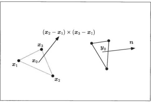
Free-Form Deformation (FFD) belongs to the group of deformation models requir ing a deformation tool, such as a lattice. A lattice is represented hy a trivariate volume regularly subdivided and deflned by a three-dimensional array of control points [201. The object that has to be deformed is embedded inside the lattice. To deform an object the user deforms the lattice by moving its control points. Any point lying inside the lattice is deformed according to the lattice deformation. In particular, the deformation of an object inside the lattice follows the dispiace ment of the lattice control points [20]. This is the unique aspect of FFD: instead of deforming the ohject directly, the object is embeclded in a space that is then deforrned and the deformation is realized in an indirect way. A good physical analogy for FFD is to consider a parallelepiped of clear, flexible plastic in which is embedded an object, or several objects, which we wish to deform [20]. The oh ject is imagined to also he flexible, so that it deforms along with the plastic that surrounds it [6]. Mathematically, the FFD is defined in terms of a tensor-product trivariate Bernstein polynomial. We begin [20] by imposing a local coordinate system on a parallelepiped region; tÏien, any point X that has (s,t, u) coordinates in this system is transformed as:

X=Xo+sS+tT+uU. (2.1)

The (s,t, u) coordinates of X cari then be found using linear algebra. For any point interior to the parallelepiped, we have O < s < 1, 0 < t < 1, 0 < u < 1 ancl a vector solution is

(TxU).(X_Xo)(UxS).(X_Xo) (SxT).(X—X0)

(TxU).S ‘ — (UxS).T (SxT)•U

(2.2) Next we impose a grid of control points P-k on the parallelepiped. These form

1 + 1 planes in the S direction, ru + 1 planes in the T direction, and n+ 1 planes

CHAPTER 2. SPATIAL DEFOR.MATION ₁₀

defined by

Pk X0 + + + U, (2.3)

t m n

vherei0,...,l,j0 ,m,andk0,...,n.

The deformation is specified by moving the Pk from their original latticial

positions. The deformed position Xffd of an arbitrary point

X

is found by first computing its (s, t, n) coordinates from equation (2.2), and then evaluating the vector

Xffd (t

)

₍

)tii

[

( )

(1- t)t

[

(

n

)

t_

fl)fl-kVkP] (2.4) where Xffd is a vector containing the Cartesiau coordinates of the deformed point, and where Pk _{is a vector containing the Cartesian coordinates of the control}

points [20].

2.2.2

FFD in our application

With the FfD method1, provided two groups of control points which form the

two control lattices (one original and one deforrned) and the poillt-based original

figure, we can get the final deformed figure.

In our application we need one extra step to get the deforrned control lattice, given the two groups of marker points (one original and one deformed) on the object. What we _{want to achieve is to choose the deformed control lattice so}

as to deforrn the whole space containing all the original marker points to either interpolate or approxirnate ail the deformed marker points. So the whole process of this method is:

1. Get the deformed control lattice:

Collstruct the original control lattice for the whole object, and get the co ordinates of ail the original control points which are just the vertices of the original control lattice. Match the trallsforrned coordinates of the original ‘The approach described here, for controllingthe FFD, is new. Itwas,however, unsuccessful,

C}IAPTER 2. SPATIAL DEFORMATION

n

marker points and that of the deforrned marker points to get the coordinates of the deformed control points, which form the deforrned control lattice, as2:

T’1’11W19... T’VM * W21I1722...1142A1 9 t.f Sq tq Uq).]3xM = [...Pr ...J3T .5) I17jr 1T’V12. T”7NA1 _{Nx M} where =

( )

(1_s)’s

[

( )

(1- t)mJti

[

( )

(1_

r= 1,...,N= (i+i)(m+i)(n+i), andq= 1,...,M; Misthenumberof control points. Here the original marker points act as the weight coefficient for the deformed control points by forming the weight inatrix. The unknowns in (2.5) are the control point P of the deformed lattice.

2. Get the final deformed figure:

Use the deformed control points to calculate the deformed coordinates of ail the points on the ob.ject using equation (2.4).

Advantages of FFD

The advantages of FFD as a method of space deformation are quite obvious. first, FFD is a representation-independent deformation technique. It can be applied not only to aiiy solid-modeling system, such as Constructive Solid Geometry (CSG) or Boundary Representation (B-rep), but also surfaces or polygonal data [20]. Second, the deformation cari be formulated in terms of any polynomial hasis, such as tensor-product B-splines or non-tensor-product Bernstein polynomials, which means the deformation can be applied either globally or locally, based on need. Each time we can choose the best and most convenient way to express the deformation. Third, the deformation method works by space deformation. This is the most important point in our application. hecause our purpose is to choose the deformed control lattice so as to deform the une (corresponding to the spine

CHAPTER 2. SPATIAL DEFORMATION 12

in the application) in the middle according to the degree of deformation of ail the points on the cylinder (corresponding to the torso in the rea.1 application). This can keep the whole deformation space continuous such that both parts can have consistent deformations.

Disadvantages of FFD

The disadvantage of the FfD method itself is that it is difficuit to control

_[81.

It is a global deformation rnethod in that it takes a space and bends it. According to [25], it works well in simple cases, but fails when complex, subtie, local deformations are required over a surface. Plus, this method requires editing a lattice to match a specific object and cleforming it to produce the desired ohject deformation. This process may prove difficult, particularly when the object’s shape does not fali into a simple combination of predefined types of lattices, and when the deformation is so complex that the correspondence between the lattice deformation and the object deformation is not straightforward [6].

The disadvantages of FFD in our applicatirn are quite crucial and finally led us to abandon this method. First, as part of our application actually we need the

inverse of the standard FFD; this requires ca.lculation of the inverse of a. matrix, or at lea.st the LU decomposition. In the either case, we have to worry about matrix singularity, especially in our application: sometimes it is quite possible that more than two original marker points lie on a une. The second disadvalltage is related to the number M of control points, which may cause (2.5) to be over- or under-determined. Also, for the methocl of FFD. the more control points we have, the hetter deformation we can get, but there is a practical constraint concerning the number of marker points (both the original ancl the deformed ones). The Iimited number of rnarker points led to part of the final deformation being out of control (in regions where there are no control points)3. The very poor resuits of our preliminary experiments with this method led us to change our research to other methods of deformation. We give a brief description of these experiments

CHAP TER 2. SPATL4L DEFORi\ÏÀTION 13

iII the next subsection.

2.2.3

Preliminary experimental resuits usirrg FFD

We hegin with the local coordillate system (s, t, n) on a parallelepiped region definied by Xo, S, T and U [20, p. 153]. There are N (1 + l)(m + 1)(n + 1) control points _Pijk defining the original control lattice grid as equation (2.3). Here we take I = ru n = 1 so that in total there are 2 . 2 2 = 8 control points.

Within this parallelepiped region, an open cylinder is defined, in terms of the

(s,t, n) coordinates (see Fig. 2.1). In the sirnplest case, this might of course just

Figure 2.1: Preliminarv test model for FFD model a blue open cylinder, which represents the deformation target (original cylinder), ernbedded inside a cube. which is the original control attice: white points represent the deforrned control points; green points represent the original marker points; red points represent the deformed marker points; gray cylinder (not shown here) will represent the deformed cylinder; the turquoise une is the original spine and the yellow une represents the defornieci Spine.

CHAPTER 2. SPATIAL DEfORMÀTION 14

be the ordillary Cartesian system:

X0 [0,0,o],S [1,o,o],T [0,1,o],U [0,0,1].

We would then like to filld new values of _Pijk for ail the points on the cylinder which will cause given rnarker poillts on the (original) open cylinder to be trans formed into given (observed) values in (s.t, ‘u)-space R3. In our experiments, we chose the number of rnarker points M = $ to simplify the calculation, since if the

number of marker poillts M is smaller thail the number of control points _{N, the} solution may lot be unique. When M is greater than N, the solutiol may not

exist at ail, and the Least Square technique lleeds to be applied. Here are sorne of our preiirninary test resuits:

1. Test case 1: Here we choose the number of marker points III = 8, move

two of the control points outward (see Fig.2.2 (a), showing the two white control points on the right side) to get some intuitive idea of how the method works. As we eau see just from the figures, the deformation works quite in the wav _{expected: one side of the lower part of the cvlinder moves out, and}

the internai vertical une switches to the side of the cylinder, which extends out a littie bit: the rest of the cylinder remains almost unchanged.

(a) (b)

figure 2.2: FFD test case 1 move two control points outward, (a) is the side

CHÂPTER 2. SPÂTIAL DEfORMÀTION 15

2. Test case 2: This is our secolld test with this model. We use the same number

of marker points, but move four of the eight control points, two outward and two inward (see Fig. 2.3). The deformatirnl resiit is pretty good. In the direction where the control points move, the object is deformed, see fig. 2.3 (b); the whole cylinder is sheared according to the upper two outward-moved coiltrol points and the lower two inward-moved coiltrol points. And, in the direction where there S 110 change in the positions of the control points, the

cylinder remains unchanged: sec Fig. 2.3 (a).

3. Problem with the FFD model. During the time we did the preliminary test

for the FFD model. we met very serions problems. which lcd us abandon this method finallv. Ilamel. there appear large distortiolls in the deforrned figure (sec Fig. 2.4).

2.2.4

Extended versions of FFD model

In spite of the disadvantages of the ffD model as we mentioned in the previous section, this method is still quite powerful. AuJ several extended versions of the

Figure 2.3: FFD test case 2 move four control points (two outward and two

illward), (a) is the view from the unchanged side; and (b) is the view from the changed side. Here. the bine cvlincler is the original cylinder and the pink one represents the deforrned one.

CHAPTER 2. SPATIAL DEfOR.MÂTIO ₁₆

basic FFD model have appeared:

1. Extended free-form deformation (Ef f D)

Extended free-form deformation; this [9] works 011 the same mathematical foundations but increases the power of the modeling system by using any shape of initial lattices or combining them [4].

2. Rational free-form deformation (RFFD)

Rational free-form deformation [13] is another extension of fFD. It allows incorporation of weights defined at each control point of the parallelepiped lattice. _{However, when the weights at each control point are unity, the}

deformations are equivalent to the FFD. To control the deformation, the user

either moves the lattice control points or modifies their associated weights.

The coordinates 0f a point are cornputed _{in the lattice parameter space} before editing the lattice control points [4].

3. Direct free-form deformation (DFFD)

Direct free-form deformation [12] is sÏightly different from the other two ex tensions. Part of this method belongs to the category of direct-manipulation deformation, but since it is also an extension of ff D, we list it here. DFfD also consist.s in embedding the object that lias to be deformed inside a trivari

figure 2.4: Problem with the fFD model: there appear large distortions in the

C}IAPTER 2. SPATIAL DEFORMATION ₁₇

ate lattice defined by an array of control points. The object deformation follows the lattice deformation but the dispiacements of the lattice control points are computed from actions such as: “move this point of the object to there” [4].

In summary, free-form deformation, extended free-form deformation, and rational free-form deformation techniques rely on the same mathematical formulation. The deformed area a.s well as the shape of the deformation inside the deforrned area depend on the polynomials. The deformed area is either the whole lattice or a part of it. To localize a deformation, the original lattice should either include a limiteci part of the object or its subdivision in chunks to be modified [4].

2.3

Direct-manipulation deformation

Direct manipulation deformation is the other group of deformation techniques. Two models belong to this group: space deformation, which will be described here, and direct free-form deformation. which vie have discussed in the previous section together with other extended versions of free-form deformation [4].

Introduced in 1991, the space deformation mode! defined of Borrel and Becli manu [7] provides direct manipulation of the object. Intermediate tools, such as lattices, are no longer required. The deformation of the object is simply specified by the dispiacement of arhitrary selected points called coristraints. The size and the boundary of a hounding box centered around each constraint point allows control of the extent of the deformation. Depending on this extent, the whole object can be included (global deformation) or only a limited area around the constraint point (local deformation). A large range of deformation shapes such a.s arbitrarily shaped bumps can be designed using this technique [4].

Chapter 3

$moothing Spiine Models

Spiine models can involve functions based on different index sets

T.

Here mainly two cases interest us:

T

— [0, 1] and

T

= Ré’.

In many practical applications, using only rigid transformations is obviously far from satisfactory, and the lack of accuracy of the resuit may cause the whole method to be useless. This makes elastic transformations, which allow for local adaptation and which are constrained to some kind of continuity or smoothness, quite attractive. Thin-Plate Spiine (TP$) is one of the methods currently being used and studied widely.

One of the goals of this thesis is to show how to adapt the TPS methods presented in the literature to our particular problem, since the link is not always obvious. This will sometimes involve generalization (for example, increasing the dimension from 2 to d, d> 2), and sometimes specialization (for example, assum ing that data observations are always paired, or, in general, “grouped d-wise”). We will also sometimes make changes to arbitrary factors (for example, multiply ing a matrix by a factor, when this change can be compensated by an arbitrary weighting factor elsewhere in the formulation). The purpose of doing this is to arrive at a similar notation for several different methods (originally presented in the literature using different formulations and notations), so that their similarities and differences can be observed.

CHAPTER 3. SPvIOOTHING SPLINE JVIODELS 19

3.1

Note on terminology

Based on the fact that certain technical terms may appear in different situations with different meanings, in this first section we make a note on terminoiogy which will help clarify the discussion in later sections.

3.1.1

Interpolation and time-interpolation

A continuous function y y() can be used to represent the n_{+ 1 data values by}

passing through ail the n+1 points Yj, i 0,. . . , n. Then one can find the value of y at any other value of x. This is interpolation, as opposed to approximation. In

our expla.nation later on, the same terrn “interpolation” has a different meaning

(interpolation as opposed to extrapolation). To differentiate these concepts, we

use “time-interpolation” for the second oiie.

3.1.2

Recapitulation

• Time-interpolation and time-extrapolation

Tirne-interpolation and time-extrapolation are two terms we used for the [0,11 index model. Tirne-interpolation refers to an estimation of a value within (viewed in the [0,1] time domain) two known values in a sequence of values. This is opposed to time-extrapolation, which is an estimation of a value based on extending a known sequence of values or facts beyond the range in [0,1] that is certaiiily known; this is often called “prediction”. • Interpolation and approximation

Interpolation and approximation are terms used for both the [0,1] index model’ and the Rd model. They are just standard terms: interpolation rep resents the _{case where the continuous function passes through all the given} points, and approximation represents the case where a smoothing parameter

‘Interpolation and approximation can be used in our application to do time-interpolation or time-extrapolation of the torso and spine, given marker points data, over a single time interval.

CHAPTER 3. SMOOTHING SPLINE MODELS 20

is introduced into the function, so that the cont.inuous function just approx imates the given set of data. The level of approximation depends on the value we choose for the smoothirig parameter. In the approximation ca.se, the form of the function usually is more smooth.

3.2

The case

_T

—

[O, Ï]

3.2.1

Mathematical outiine

The bivariate Thin-plate spiine model based on the [0,1] index set is described as [14, 24]:

yk=fk(tk)+ek,kl,2;z=l,...nk, (3.1) where the th _{response of the kt’t}

variable yj is generated hy the kt1 _{function fk} evaluated at the design point tkj plus a random error ki• Here it is assumed that

ki ‘N(O, u) for fixed k — 1, 2 ancl Corr(ci, e2)

— p if Yii and Y2j are a pair and

zero otherwise; also the domain of both functions is [0, 1] and fk E T12, where W2 =

{f: J. f’

ahsolutely continuous, f’(J11(t))2dt _<oo}

This method can be quite easily extended to multi-response data: just let k = 1, 2, ,U, where U is the dimension. In our case2, the data corresponds to the coordinates of points in space, so ungrouped data (“unpaired data” in the bivariate case) is not relevant. Therefore, here we assume the variable U (dimension) has the value 3, and that the number of observations rik and the trade-off pararneter ‘k (see below) for the three groups are the same for each k = 1,2, 3. Therefore we may then use n instead ofk and À instead ofÀk. Plus, we sometimes use x, y, z to represent the three components of each observation, which may be more intuitive for understanding of our particular application. Denote tk (tkl, ...,tkfl)T, fk ₌

(f ( \ (# T — t — t T e — (eT eT cTT

iJkk1), Jkkn)) , Yk — kYkl, «, Ykn) , — 6k1, «, kn) , — 1L ,‘2 ‘‘3 J

and (y )T where the superscript T _{refers to transpose.}

We will take 2The development in this section, showing how [21] can be adapted to our problem, is new,

CHAPTER 3. SMOOTHING SPLINE J\ÏODELS 21

the inverse of the co-variance matrix W—’ to be the direct sum of three matrices of the form

).

(3.2)

This matrix cari be obtained from the matrix W-’ in

[241

by assuming that the correlation p = O, that the matrix there is multiplied by the factor 8 o1u2, and

that the dimension has been raised from 2 to 3. The multiplicative factor cari be compensated by a change in the arbitrary constant À discussed below. In general it may be useful to permit non-zero off-diagonal elements, and different values for the aj in each of the three blocks. In this case the nine values corresponding to the jh row and the

_j’

_{column of each of the three blocks should form a 3 x 3} covariance matrix (see Section 3.3.2).

The function fk cari be estimated by solving the following penalizeci weighted

least-squares problem:

ri ri ri

min {(y-f)TW(y-f)+À

J

(f’(t))2dt+À

J

(f’(t))2dt+À] (f’(t))2dt}, (3.3)

fi,f2,f,E’i2 _o

.

_{o o}

where the first term is the weighted least-squares and the remaining terms are penalties for the roughness of the funct.ions. The parameters À control tlie trade off between goodness-of-flt and the srnoothness of the estimates and are referred to as smoothing parameters [24]. Now the solution giving the prediction function is [23]

in n

fk(t) dk(t) + ciR’(t,tk), k = 1, 2,3; (3.4)

it can be expressed in vector form as

_[

x(t),y(t), z(t)

Cxl,Cyl,Czl

[, (t),. ,.(t)] : +

[

R’(t, t1),... ,R’(t,ta)] : , (3.5) dxrn, dym, c, in which (t) = t’/(v — 1)!,v = 1,..

defines the m-dimensional space of polynomials of degree m — 1 or less, spanned

CHAPTER 3. SMOOTHING $PLINE i\/IODEL$ 22

R’(s, t) k2(s)k2(t) — k4(s — t)

where k,,,(.) = B(.)/t’!, and B is the v’th Bernoulli polynomial: B2(x) = —

x + , B4(x) = x4 — 2x3 + x2 — . The vectors

-i J ,-i ,i ,-i T [L

— kx1, ,‘xm, y1, ,‘-‘ym, z1, Uzrn)

_t

C — , Cy1, ,Cyrj, C)

which are chosen to minimize (3.3) when

f=Sc+Td. are stated in [24] to 5e the solutions3 to

f

TTWT TTWS

_f

_d

—

f

TTWy

3 6

$WT

sws

+

s

)

c) —

swy

where Tk = = 1,2,3; in our special case Tk is independent of k. Since for us the data represents the components of a position on the torso or spine, at a specific time, we have t1 t2 = t3j, (data paired, or “grouped 3-wise”) and we just use t for ail three. Here,

ç1(t1)ç59(t1) ... m(ti) i(t2)ç2(t2) ... çb(t2) 51(t) ç9(t) ... çbm(tn) çi(ti)ç9(ti) ... ç5rn(ti) ç51(t2)q2(t2) ... ç(t2) ç5rn(tn) ç51(t2)ç52(t2) ... Çrn(t) Çm(tn)

Also, S = diag($k) where _{5k = R’(tkj,} tk)l3l, k = 1,2,3, and, similarly, _$k is independent of k. Using the same simplification for tki,

R’(t1,ty)R’(t1,t2)...R’(ty,t) R1(t2,ti)R’(t2,t2) . R’(t,t,) o R’(t,t1)R’(t,2) ...R’(t,t) R’(ty,t1)R’(t1,t2)...R1(ti,t,) o R’(t2,t1)R’(t2,t2) .. R’(t1,t1)R’(t1,t2) o o R’(t2, t’) R’(t2,t2) .. R’(t2, t) R’(t,t,) R’(t,, t2) •.. R’(t,t)

and c and ci are chosen to minimize (3.3) when

3To avoid a conflict in notation in the later comparison between different methods, we changed the notations here, writing S instead of .

CHAPTER 3. SMOOTHING SPLINE JVIODELS 23

fzSc+Td.

Here

_f

is (3n x 1), S is (3nX 3n), e is (3n x 1), T is (3n x 3m), and d is (3m x 1). Then, the objective function iii (3.3) can be written

[y — (Se + Td)]TW[y — (Se+

Td)]

+ cTÀSc. (3.7)

Expanding this, dropping the term yTWy (which does not depend on e or cl), and dividing by 2 gives:

_yTwsc — YTWTd+ cT.\Sc+ cTSWTd + dTTTWTd + cTSWSc.

Differentiating with respect to e and setting the derivative to zero gives:

—SWy + [$1175 + ,\5]c + $WTd = O,

auJ differentiating with respect to U and setting the clerivative to zero gives

_TTWy + TTW$c +TTWTU _O.

These equations are exactly those of (3.6). It is also stated in [24] that a solution to

Ç

(S+M17’)c+Td=y

38

TTc=O

(.)

provides a solution to (3.6). To see this, multiply the first equation of (3.8) on the left by 8W, to obtain the second equation of (3.6). Now, multiplying the same eqilation on the left by TTW, we obtain

TTWTU + (TTWS + ÀTT)c T’Wy

which, given the second equation of (3.8), yields the first equation of (3.6). To calculate the coefficients e and U, we use the following transformations:

= S,’\O

= Àc.

CHAP TER 3. $MOOTHING SPLINE MODELS 24

If ,\ = 0, then, revising the derivation following (3.7), (3.8) will be replaced by

the single equatioll Sc + Tri y, which guarantees (3.6). These equations are apparently inconsistent for n> 2.

If ), 0, then equations (3.8) cari be expressed iII matrix-vector form as:

Xi d,1 t S1/\ O O W’ O O _\ c\ T1 o o d1 yi O 82/)i O ₊ O W,’ O ₎ cÀ ₊ O T O O O S/) _O O WZ’ J z) O O T3 _dym dz1 Z1 d7 z — T T1 O O c\ O T. O c,À = 0. (3.9) O O T c.\

Here ail the ITT_l _{I’V’. W’ are n x n matrices. Let} Tk (Qk1Qk2)( )k = 1,2,3

be the QR decomposition of Tk, a.nd let

Qi = d’iag(Qii,Q21) = d’ag(Qi2,_Q22)

R diag(R1, R2) B=+I4’. The solution finally is

_[241

c = Q2(QBQ2)’QÇy,

Rd = Q(y—B).

(3.10)

3.2.2

Permuting variables for later comparison

As illustrated in the previous section ah the matrices for the functions in the case of [0,1] index are ordered based on components, which means they are formed with the order of x, y and z coordinates in our special case. In this section we will show how these matrices can be permuted to another form which is baseci

CHAPTER 3. SMOOTHING SPLINE MODELS 25

on each single point. Our main purpose for doing this is for the later comparison of the model using [0,1] index and the model using Rd (sec Section 3.4). Ail the components in the equations

f

(S+W’)c+Tdy

311

TTcO

L

can 5e permuted to give:

1(t1)00 tli2(ti)00 m(ti)00 0,(t,)0 0ç9(t,)0 0m(ti)0 00qi(t,) 002(t,) 00m(ti) ç1(t)00 q52(t)00 ç5m(tn)00

o

,(ta)O Oç5,(t)O ... O m(tn) O 00q,(t) 0Oq52(t) O0rn(tn) R’ (t,, t,)00 R’ (t,, t,)00 R’ (t,, t11)00 OR’(t,,t,)O OR’(t,,t,)O OR’(t,,t)O

00 R’ (t,, t,) 00R’ (t,, t2) 00R’ (t,, t) R’(t,t,)00 R’(t,t,)00 R’(t,1,t)00 OR’(t,t,)O 0R’(t,t1)O .. . OR’(t,t)0

00R’(ta,t,) 00R’(ta,t9) 00R’(ta,t)

dxi C dyi Cyi Yi Y2 c= ,y: dxm cl _cyn dzm

Later on we will use this permuted version for the comparison between the [0,1] index model and the Rd index model.

3.2.3

Time-interpolation

Time-interpolation is our first application of the Thin-plate spiine model on [0,1] index. Our goal is to get some idea of what is going on in between two given states. This is especially useful in our real application scoliosis. Given the two different states of the patient body, this model can help both the doctor and the patient know how the disease changes.

CHAP TER 3. SMOOTHING SPLINE MODELS 26

With the functirni5

m n

fk(t) d(t) + cR’(t,tk),k 1,2,3,

each time we input tlie time index list and the coordinates list of one body point (a point in R3) at ail the time points to calculate the coefficient arravs c and d of this body point. Then by changing the value of t we can get its coordinate at any corresponding in-between tirne.

There is more than one choice for the time index list [t1, t2,.• , tj. First, siilce in the time-interpolation situation, only the start and the final state are invoived in the model, we coud use these two groups tStart and tend, plus the data at the closest ti;ne point, as constraints for the calculation of the deformation6. This method, appropriate in a test situation, lias the advantage that we stiil have some given data at hand with which we can do some comparison. But its shortcorning is that only using three tirne points as constraints may actually reduce the overall accuracy of the whole method (if there are more available). Because less available data involved mea.lls less information coullted. and sorne state that lias a big influence in the interpolation problem may be ignored. Another approach is to use ail the available data to do the time-interpolation, that is, ail the [t1, t2, . . . ,t] time points participate in the calculation of time-interpolation. So no matter which state is appoillted as the start state and which is the final state, each time the aigorithm uses exactiy the sarne group of data as constraints. This method is what we wouid use when working with the reai patient case. But, stili for test purposes, we ignore one group of avaiiabie data to test the accuracy of our rnethod.

Concerning the I’V’ matrix which contains the variance parameter u, in our application, we arbitrarily set ail the values of to be 1, and for the smoothing parameter ..\ which appears as part of the J474 matrix, we change it as necessary. 5For our application, ail the data are grouped: the tirne index lists are the same for ail three componentS.

6The inequality n > mis one of the conditions for the model; since m = 2, the smallest value

C’HAPTER 3. SMOOTHING SPLINE MODELS 27

As we discussed before in Section 3.2.1, in the case of [0,1] index Thin-plate spline model, interpolation, in which À 0, is impossible when in = 2.

Later in Chapter 6, we xviii show experimental resuits for this model, inciuding both the preliminary and reai-data test cases.

3.2.4

Time-extrapolation

Time-extrapolation is another application for which we tested the Tiiin-plate spiine model on the

[0.11

index set. By definition in the previous section on terminology, extrapolation is just to get something based on what we have, at some future point in time. And this is what attracts us most: prediction. The main idea under this model is to obtain, from certain groups of data, some trend information which helps us to know what xviii happen next (prediction). Applying this to our scoliosis application, the use would be quite interesting: we rnight help the doctor to do some prediction of the form of the spine at some later time point. This time-extrapolation model is not much different from the time-interpolation model since they share the same [0,1] index model. We have the time index list and coordinates list as input, and get the coefficient vectors c and d. Then each time we only need to input a value of t which represents the time point at which we want get the extrapolated figure. The only difference here is that under the time-extrapolation model, this input t is greater than 1. For testing purposes, there are two options available for the specification of the time index list. Que is simply using the original value of t xvhich is great than 1 as input, and get the coordinates of the point at the extrapolated state. The other one is to compress ail the values down within the [0,1] interval:

tj0 Z — 0,

where, tjnew is the “compressed” value of t for extrapolation, tjotd is the original value of t for the current model7, and ti tpo1d is the value of t that is greater

7Since for this method, extrapolation will use ah the available data, therefore, the time index Hst is fixed for each test case.

JHAPTER 3. SMOOTHING SPLINE MODELS 28

than 1, which represents the target tirne point. This is the method we used. Sirnilar to the time-interpolation model, there are also two ways available to get the extrapolated resuit, either based on ail the given data or only the last three data points. We chose the former one for reasons similar to those given above the time-interpolation model.

Later, in Chapter 6, we will show the experirnental resuits of this model in cluding both the preliminary and real-data test cases.

3.3

Thecasel=Rd

Our original motivation for the use of the Thin-plate spline model based on the Rd index vas to do some prediction of the internai spine information, given some marker points around the external patient body and the full point-bv-point orig inal patient body. But the real application is much more cornplicated tha.n the simple simulated test model, and there are serious problems with the real data8. We have, however, got sorne conditional good results.

3.3.1

Mathematical outiine

Interpolation

Thin-plate spline model for interpolation can be stated as a mllltivariate interpo lation problem [19]: given a number9 N of corresponding marker points p and

q, i = Ï,...N in two images of dimension cl, find a continuous transformation

u : R’ R’ within a suitahie Hilbert space H of admissible functions, which 1) minimizes a given fiinctional J : H —+ R and 2) fulfihis the interpolation

conditions

q u(p),i = 1,...,N, (3.12)

8We will discuss the problems with the real test data later on, in Chapter 6.

9To avoid a conffict with the notation n we used for the [0,1] index model, which represents the number of marker points, here we tise N for the number of inarker points.

CHAPTER 3. SMOOTHING SPLINE MODELS 29

whule minimizing the functional which represents the bending energy of a thin plate separately for each component k, k 1, ...,d

J(u) =J(nk). (3.13)

Here, the single functional is

= i+.=m iL.ad! Ldtax..a

(3.14)

The solution of minimizing the functional can be written as [19]

u(x) a(x) +wU(x,p), (3.15)

and this is tire function used for prediction. It cari also be expressed in vector

forrn as

[ux,ny,uzl

=

E

&(x),» .j(x)

]

+[ U(x,pi),... ,U(x,pN)

0Afr, UfJyapj Wj%, WNz

(3.16) The set of functions 4’, span the space 11m1_{(Rd) of ail the polnornials on R’ up} to order ‘m — 1, which is the nullspace of the functional in (3.14) [19] with values:

1(x) = 1, (x) x, 3(x) ₌ y and 4(x) z in the case m = 2. The dimension

of the space is M = and M must be not greater than N. This is because

later on, to get the solution to the prediction function, we need to have the QR decomposition of the P matrix which is of dimension N x M, so a larger value of M does not work here. The basis functions U(x,p) depend on (1) the dimension of the domain, (2) the order in of the derivatives in the functionals, and (3) the Hilbert space H of admissible functions [19, 21]. It cari be expressed as follows [19]:

—

f

m,’Jx

—p2m_dtflIX

—p, 2m — cl even positive integer

Uiz,I)j —

2m—d . 3.17

Om,dX — , otherwise.

Tire constants a = (ai, ...,aj,j)T and w _{= (‘wy,} ..., wN)T _{corresponding tire specific} colurnn in (3.16) satisfy the following system of linear equations:

CHAPTER 3. $MOOTHING SPLINE MODELS 30

Kw+Pa = y

pT

= _(3.18)

in which

U(p11p1) U(p1,p9) U(p,p)

(‘2’1) t1(P2,P2) U(p2,pT)

U(pN,pi) U(pN,p2) U(pN,pN)

and

&(p1) Ç2(Pi) ÇM(Pi)

]J= &(P2) 2(P2) çb1i(p2)

bl(pN) 2(PN) M(PN)

Now equation (3.18) can be transforrned into matrix form as:

-[‘iN qixgiyqi

‘21’22’-2N

>< W2cW2yW2z + 21P22P2M >< 2x2q2z = qixq2yq2z AN1AN2 1NJ’ï WNxWNyiVN: PN1Pjv PNJ1I aAiaMaM qNxqNyqNz

T WJiW1yWlz Pii W2xW9yW2z =

o.

(3.19) PNlPj’’2 “PNAI WN1WNyWNz Let P=(Qi:Q2)(

)

be the QR decomposition of P. The solution finally is

[231

w = Q2(QKQ2)’Qv.

Ra Qf(v — Kw).

(3.20)

Approximation

When we want to ta.ke into account landmark loca.lization errors, we just extend the basic interpolation approach hy weakening the interpolation condition. This can be achieved by introducing a quadratic approximation term in the functional

OHAPTER 3. SMOOTHING SPLINE MODELS 31

(3.13) as [19, 23]:

1 q -u(p)

+ ÀJ(u). (3.21)

The first term of the functional in (3.21), which is called the data term, measures

the sum of the quadratic Euclidean distances between the deformed marker points p and the given marker points q. Each distance is weighted by the variances

u? _{representing landmark localization errors. The second term in (3.21) measures} the smoothlless of the resuitillg transformation. The minimizatioll of the func tional yields a transformation u which (1) approximates the distance between the marker point set and (2) is sufficiently smooth. The relative weight between the approximation behavior and the srnoothness of the transformation is determined by the regularization parameter ,\ > O. If \ is small, we obtain a solution with good adaptation to the local structure of the deformations and if ,\ is large, we obtain a very smooth transformation with littie adaption to the cleformations. There are two limiting cases: for — O we obtain the original i;terpolating Thin

plate spiine transformation, and for \ — 30 we have a global polynomial of order

up to ‘rn — 1, which has no bending energy at ail [19].

The computationai scheme to compute the coefficients of the transformation u is: (K+NW’)w+Pa = u PTw ₀ (3.22) where O” I4’ .

I

. (3.23)

So now if we use K to represent K + iVV’, then we get U(p1,p2) _U(pl,pN)

U(p9,p1) ... U(p2.p1)

CHAPTER 3. SMOOTHING SPLINE MODELS 32

We get:

K11A12 1N wwYwZ P11P12 qixqiyqi:

• ‘(

+ P21P22 •Ppj

x a91a99a2- = q2xq2yq2:

AN1KN2 KNN WNxWNyWN PNYPN2 • aMa1IaM qNxqNyqNz

T P21P22•• 0. (3.24) PN1PN2 WNxWNyWNz Let P(Q1 :Q2)(

)

5e the QR decomposition of P. The solution finally is [23]

w Q2(QKQ2)’Qv,

Ra = Q(v - kw).

(3.25)

3.3.2

Anisotropic marker points

The approximation scherne descrihed in the previous section uses scalar weights to represent marker point loca.lization errors [19]. This, however, implies isotropic localization errors and is only a coarse error characterization. Generally, the errors are different in different directions and thus are anisotropic. A further extension of the approach is ohtained by replacing the scalar weights u with matrices representing anisotropic marker point Iocalization errors [19]. Now the functional is:

Jo)

= 1

— u(q) )T1

(

— u(q)) + ÀJ(u). (3.26)

But the computational scheme to compute the coefficients of the transformation u is the same as before:

(K+N1\W’)w+Pa = u

PTw = 0;

C1HAPTER 3. $MOOTHING $PLINE MODELS 33

the only change here is concerning the W’ matrix which becomes:

‘‘=

I

..

I.

(3.28)

N)

Note’° that the Zj represent the localization errors of two corresponding marker points. A typical Z1 in (3.26) will be a 3 x 3 symmetric, positive-definite matrix with real eigenvalues and This corresponds to using a norm that has a unit sphere in the shape of an ellipsoid. The principal axes of this ellipsoid

are n’ n2 and n3, the eigenvectors of ‘. The half-length of the ellipsoid in the

direction n is u,

j

= 1,2,3.

A large value of u means that the error in this direction is unimportant. $o if it is only the error in the direction w that is important, we would choose a pancake-shaped ellipsoid with w as the normal to the surface of the pancake. $imilarly, if it is the error in the directions u and w that are important, we would choose a long thin ellipsoid with major axis equal to u x w.

The matrix Z’ lias an orthonormal basis of eigenvectors &, n2 and n3.

O0

= [n’ n2 n3]. O O . [n’ n2 n3ÏT

OO where n 1,

j

= 1,2,3.

Since after introdllction of the matrix j, the value of errors on each direction changed according to different values in the matrix, we must make a minor modification on the overall data structure. That is, the dimension ofw is dN x 1, cz is UM x 1, and q is dN x 1. Now the modified version is:

qiz

[g].

: :

WNx aMs Nx

WNy qNy

WNz aMz Nz

CHAPTER 3. SMOOTHING SPLINE MODELS 34 and w’x ‘w’2 w1z [p]T =0, (3.29) WNx WN2 WNZ where

k

= (K + NÀW’), i.e,

N.\E1, N)I9 NÀZI3 1(12 0 0 ‘fiN O O

NÀ1 N,\Z9 NM3 O K12 O O K, O

]V)E’ AT) _{NM3 O O K12 O O KYN}

K21 O O NÀ1 N?2 N?3 K2N O O O K21 O N1 N,\Z9 NÀ3 O KSAr O K O O 1(2 NZ1 N)9 N,\Y3 O O K2N KN1 O O KN2 O O N,\ NÀZ NÀ O K O O K O NÀZ N,\EC N,\ O O K O O KN2 N2 N,\ZÇ NÀ and 11 (Pi) O O ç52(p1) O O ,5ii(î) O O O i(p1) O O ç52(p1) O ... O ii(i) O

o

o

q,(p1) O O _5(p1) O O _&ii(Pi) 1(P2) O O 12(p9) O O q5,,j(p9) O O O ç5,(p9) O O çb2(p2) O O _k’’(p) O

o

o

i(P2) O O ç(p2) O tIJ(P2) (pfl) O O ç52(p) O O _j,i(p) O O O i(p) O O 2(p) O ... O çji(p) O O O q,(p) O O _(p) O O f/iAi(p)

Here, the are the components of j, 1 <in,n < 3. Let

P=(Q, :Q2)(

)

be the QR decomposition of P. The solution finally is

_[191

w =

Q2(QkQ2)’Qv,

Ra = Q(v —

kw).

(3.30) In the implementation, it was stiil possible for us to keep the same data struc turc for this anisotropic marker points case and this will be a memory-saving

CHAPTER 3. $MOOTHING $PLINE 1/IODELS 35

technique. We cari store the error direction information in an independent matrix called LW’

Z,, Z12 Z,3 = Z2, ₂₂ Z23 Z3, Z32 Z33

then what we ueed to do is some more additious based ou what we get for the

two previous models (interpolation and approximation) as:

Zanisotropic = (Z,, x x + Z,2 X + Z,3 x z) +_‘otd;

Yanisotropic = (Z21 x x + Z22 x y + Z23 x z) + _yotd;

zanisotropic (Z3, x x + Z32 x y + Z33 X z) + z0tu.

where X01d, Yotd and z0td represent the coordinates before change, that is used for both the interpolation and approximation case, and 1anjsotropjc, Yanisotropic and

zanisotropic represent the transformed anisotropic values of the coordinates.

3.4

Comparison between [0,1] index model and

R’

index model

Que of the goals of this thesis was to show the link between the Thin-plate spline models based on [0,1] index and R’ index”. Even though they are two completely different spline models, after the permutation of variables donc in Section 3.2.2 and the mathematical development in Section 3.2 and 3.3, we can sec that they really share something in common, which is quite useful in our application.

3.4.1

Similarities

Both the [0,1] index model and the R’ model can act as prediction functions. The objective function of the [0,1] index model cari be written as

n d ₁

- f(t))TZ’(y - f(t)) + À

f

(f’(t))2dt, (3.31)

i=1 k=1 O

CHAPTER 3. SMOOTHING SPLINE MODEL$ 36

where

y — f(t) ₌ [Yii — f1(t),Y2i — f2(t),3j

— f3(t)]T

Then the spiine model based on [0,1] index model may now be easily compared with the R° model which is, for k 1, ...,d

Uk(X) = + wkU(x,p), (3.32)

by minimizing the functional

— u(pj))T(qj — li(pj)) + . i(’U), (3.33) where d ni!

f

8it 2 jm(i) ₌

_L

X

jRd

aXr...aXd

Comparing (3.31) alld (3.33), the methods have very similar structure.

It is easy to verify that, after permutation of variables, the (nd x nid) matrix

T for the [0,1] index model has exactly the same form as each (n x ni) matrix Tk, with each element (t) replaced by ,(t) . I(dxd), where I is the identity matrix.

$imilarly, the (nd x nd) matrix $ has exactly the same form as each (n x n)

matrix $k, with each element R’(t,t) replaced by R’(t,t) Analogous statements apply to the matrices involved in the equations to be solved the R” model [19], and they may be solved using the QR approach.

3.4.2

Differences

Since the [0,1] index model and the Rd index model are two different models, some differences are obvions: for example, the different definition of the coefficient vec tors for (3.31) and (3.33). But here, what interests 115 most is the relation between different body points in the model. For the [0,1] index model, the deformation of each point is only related to its own position at different time points: there is no interactive relation between points. For the R’ index model, the deforma tion is defined by the relation between body points and the marker points. The deformed position of a certain body point is decided by the positions of ah the

CHAPTER 3. $MOOTHING SPLINE 1’vIODEL$ ₃₇

marker points and the weighting factor of the distance of this body point from ail the marker points. This expla.ins why the coefficient vector generaiization test (in Section 6.3) can work with the Rd index model, while for the [0,1] index model, it does not.