Predicting image influence on visual saliency distribution: the focal and ambient dichotomy

(1)

HAL Id: hal-02530175

https://hal.inria.fr/hal-02530175

Submitted on 3 Apr 2020

HAL is a multi-disciplinary open access

archive for the deposit and dissemination of

sci-entific research documents, whether they are

pub-lished or not. The documents may come from

teaching and research institutions in France or

abroad, or from public or private research centers.

L’archive ouverte pluridisciplinaire HAL, est

destinée au dépôt et à la diffusion de documents

scientifiques de niveau recherche, publiés ou non,

émanant des établissements d’enseignement et de

recherche français ou étrangers, des laboratoires

publics ou privés.

Predicting image influence on visual saliency

distribution: the focal and ambient dichotomy

Olivier Le Meur, Pierre-Adrien Fons

To cite this version:

Olivier Le Meur, Pierre-Adrien Fons. Predicting image influence on visual saliency distribution: the

focal and ambient dichotomy. ETRA, Jun 2020, Stuttgart, Germany. �10.1145/3379156.3391362�.

�hal-02530175�

(2)

Predicting image influence on visual saliency distribution:

the focal and ambient dichotomy

OLIVIER LE MEUR and PIERRE-ADRIEN FONS,

Univ Rennes, CNRS, IRISA, France

The computational modelling of visual attention relies entirely on visual fixations that are collected during eye-tracking experiments. Although all fixations are assumed to follow the same attention paradigm, some studies suggest the existence of two visual processing modes, called ambient and focal. In this paper, we present the high discrepancy between focal and ambient saliency maps and propose an automatic method for inferring the degree of focalness of an image. This method opens new avenues for the computational modelling of saliency models and their benchmarking. CCS Concepts:• Computing methodologies → Machine learning.

Additional Key Words and Phrases:visual fixatios, focal, ambient, saliency

ACM Reference Format:

Olivier Le Meur and Pierre-Adrien Fons. 2020. Predicting image influence on visual saliency distribution: the focal and ambient dichotomy. 1, 1 (April 2020), 9 pages. https://doi.org/10.1145/nnnnnnn.nnnnnnn

1 INTRODUCTION

When looking at complex visual scenes, we perform in average 4 visual fixations per second. This dynamic exploration allows selecting the most relevant parts of the visual scene and bringing the high-resolution part of the retina, the fovea, onto them. To understand and predict which parts of the scene are likely to attract the gaze of observers, vision scientists classically rely on two groups of gaze-guiding factors: low-level factors (bottom-up) and observers or task-related factors (top-down). From these factors, computer vision scientists have designed computational models of visual attention aiming to predict the areas of an image that would draw our attention. Generally speaking, these models produce from an input image a 2D grayscale saliency map indicating the most visually interesting parts of the scene.

Since the first saliency models dating back to the 1990s, the ability to predict where we look at has greatly improved [Borji and Itti 2013; Bruce and Tsotsos 2009; Itti et al. 1998; Le Meur et al. 2006]. The very last generation of models, relying on deep networks, has even brought a new momentum in this field of research [Cornia et al. 2016a; K¨ummerer et al. 2014, 2016; Pan et al. 2017, 2016]. Beyond the fact that saliency models are becoming more and more sophisticated and powerful, it is interesting to note that the evaluation protocol has evolved only little since the 1990s. The main modification concerns the metrics used to evaluate the degree of similarity between predicted and human saliency maps [Le Meur and Baccino 2013; Authors’ address: Olivier Le Meur, olemeur@irisa.fr; Pierre-Adrien Fons, pierre-adrien.fons@irisa.fr, Univ Rennes, CNRS, IRISA, P.O. Box 1212, Rennes, France.

Permission to make digital or hard copies of all or part of this work for personal or classroom use is granted without fee provided that copies are not made or distributed for profit or commercial advantage and that copies bear this notice and the full citation on the first page. Copyrights for components of this work owned by others than ACM must be honored. Abstracting with credit is permitted. To copy otherwise, or republish, to post on servers or to redistribute to lists, requires prior specific permission and/or a fee. Request permissions from permissions@acm.org.

(3)

Riche et al. 2013]. Regarding the computation of human saliency maps, the process consists of only a few steps: first we collect raw eye tracking data. Then, the sequence of raw gaze points is translated into an associated sequence of fixations [Salvucci and Goldberg 2000]. The set of spatial locations of the fixations for a given stimulus constitutes a fixation map, which is then convolved with a gaussian filter to obtain a continuous saliency map [Le Meur and Baccino 2013; Wooding 2002]. This method assumes that all fixation points are of similar importance and have the same visual function.

However, in 2005, [Unema et al. 2005] suggested that larger saccade amplitudes and shorter fixation durations during the early viewing period represented ambient processing and that smaller saccade amplitudes and longer fixation durations during the later viewing period represented focal processing. The focal attention mode would be used to gather more detailed information thanks to the high density of cones in the central visual field. This would allow for better subsequent recognition of objects. On the other hand, ambient mode would serve to extract information from peripheral vision [Trevarthen 1968] to ease further scene exploration and to gather low-resolution but global information located at a higher visual eccentricity.

In the context of computational visual attention modelling, the focal/ambient dichotomy is clearly overlooked. We believe the distinction between focal and ambient fixations might be of a great importance for saliency prediction, in the definition and curation of eye-tracking datasets as well as for benchmarking saliency models. In this vein, [Follet et al. 2011] provided evidence that pre-deep learning era saliency models relying only on low-level visual features are better at predicting focal saliency maps than ambient ones.

In this paper, we present methods for identifying focal and ambient fixations. We then compute focal and ambient saliency maps by using several eye-tracking datasets and analyse their main characteristics. We then qualify those datasets in terms of the number of focal and ambient images.Our main objective is to provide new insights into the characterization of focal and ambient images as well as to design a method for predicting the focalness of an image. This method might prove helpful to select images for modelling the focal and/or the ambient processing modes.

The paper is organized as follows. Section 2 describes existing methods for identifying focal and ambient fixations. In Section 3, we present the difference between focal and ambient saliency maps as well as the degree of focalness of several eye-tracking datasets. Section 4 introduces an automatic method for inferring the focalness of an image. The last section presents the perspectives of this study.

2 METHODS FOR IDENTIFYING FOCAL AND AMBIENT FIXATIONS

To the best of our knowledge, there exist only three methods to label the visual fixations as being either focal or ambient.

In 2011, [Pannasch et al. 2011] perform the classification on the basis of the prior saccade amplitude, and refined Unema et al.’s definition. If the preceding amplitude is larger than 5∘, this fixation is presumably in the service of the ambient attention mode; otherwise the fixation is assumed to belong to the focal attention mode. Authors emphasize that 5∘of visual angle correspond to the parafoveal region where the visual acuity is still good [Wyszecki and Stiles 1982].

[Follet et al. 2011] investigate the fixation labelling thanks to a k-means clustering method and by using the fixation duration as well as the prior amplitude saccade. The two-classes clustering results, i.e. focal and ambient, showed that the relevant dimension is the amplitude of saccades. Over four categories of visual scenes, containing very few objects, the centers of focal and ambient centroids are in average 2.5∘and Manuscript submitted to ACM

(4)

Predicting image influence on visual saliency distribution:

the focal and ambient dichotomy 3

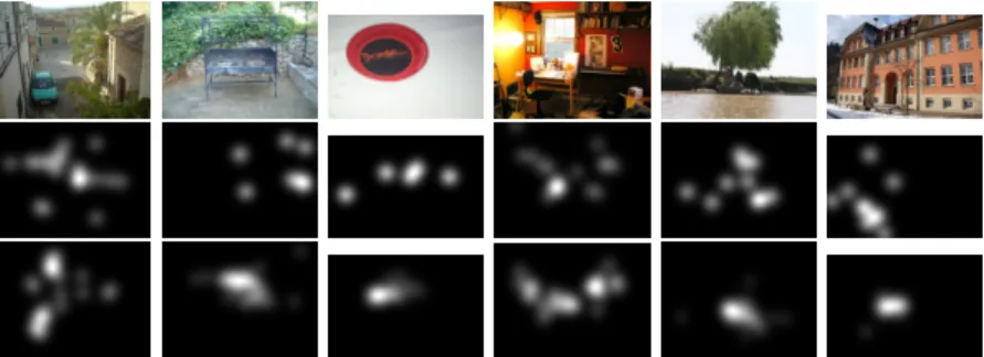
Fig. 1. From Top to Bottom: original images; ambient maps; focal maps.

10.5∘degrees of visual angle respectively. A threshold of 6.5∘was then used to label the visual fixations straightforwardly. The difference with Pannasch et al.’s results could be explained by the experimental procedure. However, Pannasch et al.’s findings are supported by Follet et al.’s results. First, the important dimension to cluster visual fixations is the prior saccade amplitude. Second, both studies observed much more focal fixations than ambient ones. For Follet et al., an average of 70% of focal and 30% of ambient fixations were observed. This distribution is consistent with the supposed role of ambient and focal attention modes.

In 2014, [Krejtz et al. 2014] define the 𝒦 coefficient to distinguish between ambient and focal fixations by considering the definition formerly given by [Velichkovsky et al. 2005]. Ambient attention is characterized by relatively short fixations followed by high amplitude saccades, whereas focal attention is described by long fixations followed by saccades of low amplitude. From this definition, the 𝒦 coefficient is calculated as the mean difference between standardized values of each saccade amplitude (𝑎𝑖+1) and the preceding fixation

duration (𝑑𝑖): 𝒦 = _𝑁1 ∑︀𝑁𝑖=1𝒦𝑖, where 𝒦𝑖 = 𝑑𝑖 −𝜇_𝑑 𝜎𝑑 −

𝑎𝑖+1−𝜇𝑠

𝜎𝑠 (𝒦 > 0, relatively long fixations followed

by short saccade amplitudes are labelled focal; 𝒦 < 0, relatively short fixations followed by long saccade amplitudes are labelled ambient). Although interesting, authors do not go further in the characterization of focal and ambient fixations. They used the 𝒦 coefficient as an indicator of the cognitive strategies occurring in a visual search.

In this paper, we perform the labelling of fixations according to the previous saccade amplitude, with a fixed threshold of 5∘, as in [Pannasch et al. 2011].

3 FOCAL AND AMBIENT MAPS

The analysis is first performed on the MIT1003 dataset [Judd et al. 2009], composed of images of various contents. We expect to observe a balanced proportion of focal and ambient images. The analysis is then extended to other datasets.

3.1 MIT1003 dataset

Example of focal and ambient saliency maps. Focal and ambient saliency maps are computed following the method proposed in [Le Meur and Baccino 2013]. For the focal (resp. ambient) maps, the focal (resp. ambient) fixations are considered. Figure 1 illustrates samples of saliency maps computed from ambient Manuscript submitted to ACM

(5)

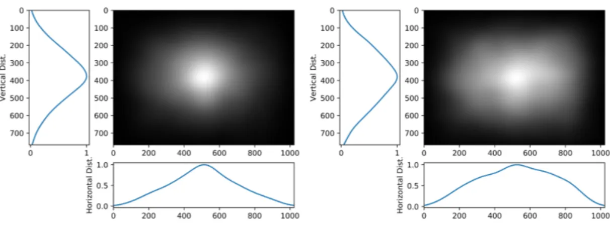
Fig. 2. Horizontal / vertical saliency distribution: focal fixations and ambient fixations.

and focal fixation maps. As expected, the saliency density in focal maps is concentrated in a few locations whereas it is much more scattered in ambient maps.

Attentional synchrony. As in [Breeden and Hanrahan 2017], we evaluate the size of the screen region attended to as the area of the convex hull of all focal and ambient fixation points. Smaller values indicate increased attentional synchrony [Smith and Mital 2013] whereas higher values would indicate a higher dispersion between observers. We expect to observe higher congruency for focal fixations. The median convex hull area is 15% and 17% for the focal and ambient fixations, respectively. The observed difference is statistically significant, paired t-test, 𝑝 ≪ 0.001. This is consistent with our expectation, given the definition of focal and ambient attention modes.

Spatial bias. Figure 2 illustrates the average focal and ambient maps computed from all visual fixations on all stimuli, respectively; note that the average of classic saliency maps is not shown. The marginal normalized distributions of horizontal and vertical salience are plotted on the bottom and the left-hand side, respectively. Several observations can be made. First we compute the degree of similarity between those distributions with the symmetrized Kullback-Leibler divergence, noted 𝑠𝐾𝐿. We got 𝑠𝐾𝐿 = 0.0075 between saliency and focal maps, 𝑠𝐾𝐿 = 0.0417 between saliency and ambient maps and 𝑠𝐾𝐿 = 0.0372 between focal and ambient maps. The lowest score (i.e. the highest similarity) is observed between the distributions of saliency maps (all fixations) and focal maps. This is not surprising since most visual fixations are focal (about 70%). We also observe that there is a strong center bias, both horizontally and vertically, for both saliency and focal maps. While mostly centered, the average ambient map is, however, much more horizontally spread out than the saliency and focal maps.

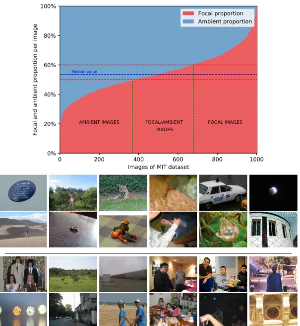
Proportion of focal fixations. We observe on the MIT1003 dataset that the proportion of focal fixations significantly varies from one image to another. Some images are clearly focal while others are clearly ambient. Figure 3 (Top) presents the amount of focal and ambient fixations per image. Images are ranked according to their proportion of focal fixations. The median value of focal fixations per image is 53%. Figure 3 (Bottom) illustrates the most focal and ambient images in the MIT1003 dataset. Focal images are composed by Manuscript submitted to ACM

(6)

few, compact and rather small objects (or salient areas). We also observe that these images often contain semantic, more abstract information, such as text. Conversely, ambient images contain either several salient objects that are spatially distant from one another or no particularly salient objects. For instance, some ambient images contain several faces. In this case, observers have to make quite long saccades to jump from one face to another in order to get as much information as possible. The absence (or the abundance) and variety of visual information in ambient images may explain that ambient saliency maps are more scattered than focal maps.

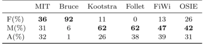
Table 1. Focal (F), Mixed (M) and Ambient (A) images in six existing datasets.

MIT Bruce Kootstra Follet FiWi OSIE

F(%) 36 92 11 0 13 26

M(%) 31 6 62 62 47 42

A(%) 32 1 26 38 39 31

3.2 Extension to other datasets

According to observations made on MIT1003, we label an image as being focal when the proportion of focal fixations is greater than 60%, and ambient when this proportion is below 50%. Between 50% and 60%, we consider that there is a mixture of focal and ambient fixations. From this thresholding, we evaluate the number of focal, focal/ambient and ambient images in existing eye-tracking datasets such as Bruce [Bruce and Tsotsos 2009], Kootstra [Kootstra et al. 2011], Follet [Follet et al. 2011], FiWi [Shen and Zhao 2014] and OSIE [Xu et al. 2014]. From Table 1, we can draw the following observations: Bruce dataset is mainly composed of focal fixations suggesting that this dataset mainly consists of focal images. Follet dataset1 is the dataset having the less focal fixations. It contains a majority of mixed and ambient images. One specificity of this dataset is that the images were selected to present empty landscapes with very few and non-salient objects. The only objects in these scenes are congruous with their surroundings such as parked cars in street scenes or trees in open-country images. Kootstra and FiWi datasets are quite well balanced in terms of focal and ambient fixations. MIT1003 and OSIE datasets encompass images with a very high and very low number of focal fixations. They gather a balanced mix of ambient, focal and mixed images.

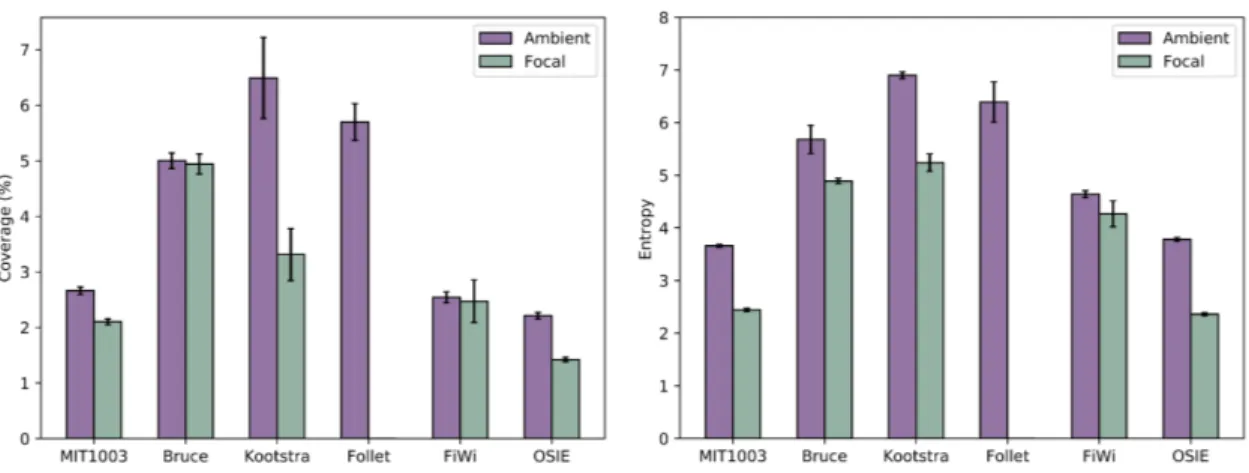
Qualitatively speaking, this straightforward classification allows to perform a clear distinction between human saliency maps, as illustrated by Figure 1. Again, focal images are associated with a much less scattered saliency density than ambient images, with a majority of the density concentrated on a few locations. If we simply threshold the focal, ambient and focal/ambient maps with a fixed threshold equal to 128, the coverage value, i.e. the ratio between the number of pixels above the threshold and the total number of pixels, reveals that focal images have the smallest coverage whereas the ambient ones have the highest (see Figure 4 (left)). On the same figure, the entropy for ambient and focal maps is also reported; as expected, the entropy of ambient maps is higher than the entropy of focal maps.

It appears to us fundamental to know whether an image is more or less focal to qualify eye-tracking datasets.

1_{Available on the following link, http://www-percept.irisa.fr/software/}

(7)

Fig. 3. (Top) Focal fixations proportion per image of MIT1003 (ranked in increasing order). (Bottom) The most focal & the most ambient images.

4 IMAGE FOCALNESS INFERENCE

A focal image is an image for which observers focus on a few specific areas. We define the image focalness as being a positive score in [0, 1]; this score is directly related to the proportion of focal fixations. A pure focal image would have a focalness of 1, a pure ambient image would have a score of 0. Our aim is here to predict in an automatic manner the focalness score of an image.

(8)

Fig. 4. Focal/ambient maps coverage and entropy.

For that purpose, we define a simple network based on the VGG19 [Simonyan and Zisserman 2014] deep network, pre-trained with ImageNet [Deng et al. 2009]. It is used as a feature extractor, where the last fully connected layers dedicated to the classification task have been removed. On top of this network, we add a shallow network dedicated to the regression task, with a 2D global average pooling to get an unique feature vector and three fully connected layers with ReLU activations, composed of 128, 64 and 1 units, respectively. Between these layers, two dropout layers are added with a dropout rate of 0.3 and 0.25, respectively.

The training is performed in two steps. First, the fully connected layers are pre-trained during a fixed number of epochs while the VGG19 extractor is frozen. Then, the last three layers of VGG19 are fine-tuned with a reduced learning rate along with the shallow regression network. We use the mean absolute error as a loss function and an Adam optimizer.

The training dataset is composed of 4192 images coming from the pooling of the aforementioned datasets to which we add images from CAT2000 [Borji and Itti 2015]. To augment data, all images are flipped horizontally and randomly undergo a brightness or contrast filtering. As the distribution of focalness scores is centered around 0.5, an over and under-sampling techniques are used to get a more balanced training dataset. We allocate 80% of these images for the training, 10% for the validation and 10% for the testing.

The Pearson correlation between ground truth and predicted values is 0.763, 𝑝 ≪ 0.01. The standard error is 0.26. Figure 5 illustrates the scatter plot of the ground truth and predicted scores. On the top-right, the prediction error histogram is plotted. Most errors belong to the range [−0.1, 0.1]. On the bottom, examples of images associated with their actual and predicted focalness scores are given.

5 CONCLUSION AND PERSPECTIVES

In this paper, we study focal and ambient saliency map characteristics. We also show that current eye-tracking datasets, which are a key ingredient for modelling and benchmarking saliency models, are not well balanced in terms of focal and ambient images. We then believe that, to go further into the computational modelling of visual attention, it is necessary to disentangle focal and ambient fixations. By extension it would be beneficial to determine the focalness score of an image before designing eye-tracking datasets and before Manuscript submitted to ACM

(9)

(c) (0.22;0.26) (d) (0.47;0.50) (e) (0.53;0.54) (f) (0.81;0.68) Fig. 5. (Top) scatter plot of the ground truth (GT) and predicted focalness scores (S) (left); Prediction error histogram (right). (Bottom) Examples of prediction with scores (GT,S).

training computational models. In this context, we have designed a model for predicting the focalness of an image. This opens a number of new avenues. Thanks to such prediction, it becomes possible to define focal, ambient or mixed eye-tracking datasets, to re-train deep learning-based models and to improve saccadic models (such as [Boccignone and Ferraro 2004, 2011; Coutrot et al. 2018; Le Meur and Coutrot 2016; Le Meur and Liu 2015]) by considering focal, ambient or mixed fixations.

REFERENCES

G. Boccignone and M. Ferraro. 2004. Modelling gaze shift as a constrained random walk. Physica A: Statistical Mechanics and its Applications 331 (2004), 207 – 218. https://doi.org/10.1016/j.physa.2003.09.011

G. Boccignone and M. Ferraro. 2011. Modelling eye-movement control via a constrained search approach. In EUVIP. 235–240. A. Borji and L. Itti. 2013. State-of-the-art in Visual Attention Modeling. IEEE Trans. on Pattern Analysis and Machine

Intelligence 35, 1 (2013), 185–207.

Ali Borji and Laurent Itti. 2015. CAT2000: A Large Scale Fixation Dataset for Boosting Saliency Research. CVPR 2015 workshop on ”Future of Datasets” (2015). arXiv preprint arXiv:1505.03581.

Katherine Breeden and Pat Hanrahan. 2017. Gaze data for the analysis of attention in feature films. ACM Transactions on Applied Perception (TAP) 14, 4 (2017), 23.

N.D.B. Bruce and J.K. Tsotsos. 2009. Saliency, attention and visual search: an information theoretic approach. Journal of Vision 9 (2009), 1–24.

Zhaohui Che, Ali Borji, Guangtao Zhai, and Xiongkuo Min. 2018. Invariance analysis of saliency models versus human gaze during scene free viewing. arXiv preprint arXiv:1810.04456 (2018).

(10)

Marcella Cornia, Lorenzo Baraldi, Giuseppe Serra, and Rita Cucchiara. 2016a. Multi-level Net: A Visual Saliency Prediction Model. In European Conference on Computer Vision. Springer, 302–315.

Marcella Cornia, Lorenzo Baraldi, Giuseppe Serra, and Rita Cucchiara. 2016b. Predicting human eye fixations via an LSTM-based saliency attentive model. arXiv preprint arXiv:1611.09571 (2016).

Antoine Coutrot, Janet H Hsiao, and Antoni B Chan. 2018. Scanpath modeling and classification with hidden Markov models. Behavior research methods 50, 1 (2018), 362–379.

Jia Deng, Wei Dong, Richard Socher, Li-Jia Li, Kai Li, and Li Fei-Fei. 2009. Imagenet: A large-scale hierarchical image database. In 2009 IEEE conference on computer vision and pattern recognition. Ieee, 248–255.

B. Follet, O. Le Meur, and T. Baccino. 2011. New insights into ambient and focal visual fixations using an automatic classification algorithm. i-Perception 2, 6 (2011), 592–610.

L. Itti, C. Koch, and E. Niebur. 1998. A model for saliency-based visual attention for rapid scene analysis. IEEE Trans. on PAMI 20 (1998), 1254–1259.

T. Judd, K. Ehinger, F. Durand, and A. Torralba. 2009. Learning to predict where people look. In ICCV. IEEE.

G. Kootstra, B. de Boer, and L.R.B. Schomaler. 2011. Predicting eye fixations on complex visual stimuli using local symmetry. Cognitive Computation 3, 1 (2011), 223–240.

K. Krejtz, A. Duchowski, and A. Coltekin. 2014. High-Level Gaze Metrics From Map Viewing: Charting Ambient/Focal Visual Attention. In the 2nd International Workshop on Eye Tracking for Spatial Research, Vienna, Austria. Matthias K¨ummerer, Lucas Theis, and Matthias Bethge. 2014. Deep gaze i: Boosting saliency prediction with feature maps

trained on imagenet. arXiv preprint arXiv:1411.1045 (2014).

Matthias K¨ummerer, Thomas SA Wallis, and Matthias Bethge. 2016. DeepGaze II: Reading fixations from deep features trained on object recognition. arXiv preprint arXiv:1610.01563 (2016).

O. Le Meur and T. Baccino. 2013. Methods for comparing scanpaths and saliency maps: strengths and weaknesses. Behavior Research Method 45, 1 (2013), 251–266.

Olivier Le Meur and Antoine Coutrot. 2016. Introducing context-dependent and spatially-variant viewing biases in saccadic models. Vision research 121 (2016), 72–84.

O. Le Meur, P. Le Callet, D. Barba, and D. Thoreau. 2006. A coherent computational approach to model the bottom-up visual attention. IEEE Trans. On PAMI 28, 5 (May 2006), 802–817.

Olivier Le Meur and Zhi Liu. 2015. Saccadic model of eye movements for free-viewing condition. Vision research 1, 1 (2015), 1–13.

Junting Pan, Cristian Canton, Kevin McGuinness, Noel E O’Connor, Jordi Torres, Elisa Sayrol, and Xavier Giro-i Nieto. 2017. Salgan: Visual saliency prediction with generative adversarial networks. arXiv preprint arXiv:1701.01081 (2017). Junting Pan, Elisa Sayrol, Xavier Giro-i Nieto, Kevin McGuinness, and Noel E O’Connor. 2016. Shallow and deep convolutional

networks for saliency prediction. In Proceedings of the IEEE Conference on Computer Vision and Pattern Recognition. 598–606.

Sebastian Pannasch, Johannes Schulz, and Boris M Velichkovsky. 2011. On the control of visual fixation durations in free viewing of complex images. Attention, Perception, & Psychophysics 73, 4 (2011), 1120–1132.

Nicolas Riche, Matthieu Duvinage, Matei Mancas, Bernard Gosselin, and Thierry Dutoit. 2013. Saliency and human fixations: state-of-the-art and study of comparison metrics. In Proceedings of the IEEE international conference on computer vision. 1153–1160.

Dario D Salvucci and Joseph H Goldberg. 2000. Identifying fixations and saccades in eye-tracking protocols. In Proceedings of the 2000 symposium on Eye tracking research & applications. ACM, 71–78.

Chengyao Shen and Qi Zhao. 2014. Webpage Saliency. In ECCV. IEEE.

Karen Simonyan and Andrew Zisserman. 2014. Very deep convolutional networks for large-scale image recognition. arXiv preprint arXiv:1409.1556 (2014).

Tim J Smith and Parag K Mital. 2013. Attentional synchrony and the influence of viewing task on gaze behavior in static and dynamic scenes. Journal of vision 13, 8 (2013), 16–16.

Colwyn B Trevarthen. 1968. Two mechanisms of vision in primates. Psychologische Forschung 31, 4 (1968), 299–337. Pieter JA Unema, Sebastian Pannasch, Markus Joos, and Boris M Velichkovsky. 2005. Time course of information processing

during scene perception: The relationship between saccade amplitude and fixation duration. Visual cognition 12, 3 (2005), 473–494.

Boris M Velichkovsky, Markus Joos, Jens R Helmert, Sebastian Pannasch, et al. 2005. Two visual systems and their eye movements: Evidence from static and dynamic scene perception. In Proceedings of the XXVII conference of the cognitive science society. Citeseer, 2283–2288.

David S Wooding. 2002. Fixation maps: quantifying eye-movement traces. In Proceedings of the 2002 symposium on Eye tracking research & applications. ACM, 31–36.

Gunter Wyszecki and Walter Stanley Stiles. 1982. Color science. Vol. 8. Wiley New York.

(11)

Juan Xu, Ming Jiang, Shuo Wang, Mohan S Kankanhalli, and Qi Zhao. 2014. Predicting human gaze beyond pixels. Journal of vision 14, 1 (2014), 28–28.