Variational Multiframe Restoration of Images
Degraded by Noisy (Stochastic) Blur Kernels
Miyoun Jung, Antonio Marquina, and Luminita A. Vese? Department of Mathematics, University of California,
Los Angeles, CA 90095, U.S.A.
Departamento de Matematica Aplicada, Universidad de Valencia, Burjassot, Spain 46100.
Abstract. We wish to recover an original image u from several blurry-noisy versions fk, called frames. We assume a more severe degradation
model, in which the image u has been blurred by a noisy (stochastic) point spread function. We consider the problem of restoring the degraded image in a variational framework. Since the recovery of u from one sin-gle frame f is a highly ill-posed problem, we propose two minimization problems based on the multiframe approach introduced for image super-resolution by Marquina-Osher [28]. Several experimental results for grey-scale and color image restoration are shown, together with binary image segmentation of noisy-blurry data and restoration of static videos, illus-trating that the proposed models give visually satisfactory results.
Keywords: image restoration, noisy blur kernel, energy minimization, regulariza-tion, multiframe model.
1
Introduction
Let Ω denote an open bounded set on which the image intensity function u :
Ω → R is defined. The standard linear degradation model for a blurry-noisy
image f is given by f = K ∗ u + n, where f is the observed image, K is a known linear and space-invariant blurring kernel, u is the ideal image, and n is additive noise, independent of u. One approach to the image restoration problem is within the variational framework, considering the minimization problem
min
u {Φ(f − K ∗ u) + Ψ (|∇u|)} ,
(as in [14, 15, 36]). Here, the functional Φ(·) is a data-fidelity term that forces the smooth image K ∗ u to be close to the observed image f , while Ψ enforces a smoothness constraint on u, and can be seen as a regularizer in the ill-posed
?Research supported by the National Science Foundation Grants DMS-0312222,
DMS-0714945, by a UCLA Faculty Research Grant 2009-2010, and by the Span-ish Government Agency Grant DGI-CYT MTM2008-03597.
deconvolution problem. For example, for Gaussian noise n, a well-known edge-preserving image recovery model was proposed by Rudin-Osher [35, 36]: assum-ing f ∈ L2(Ω), K linear and continuous on L2(Ω), their model is
min u ½ λ 2 Z Ω (f − K ∗ u)2dx + Z Ω |∇u|dx ¾ , (1)
where λ > 0 is a parameter and T V (u) = RΩ|∇u|dx is the total variation of u ∈ W1,1(Ω) ⊂ BV (Ω).
We consider in this paper a different degradation model with a noisy blur kernel inspired by [38], [40–42, 11, 19, 20, 1–4, 30]
f = (K + s) ∗ u + n,
where K is a known blurring kernel (e.g. a Gaussian function), s is unknown additive Gaussian noise of zero mean (making K noisy), and n is another un-known additive Gaussian noise of zero mean. Both s and n are assumed to be statistically independent, and uncorrelated with u. Thus, the known blur kernel
K is contaminated by noise s, producing a “stochastic point spread function”.
The stochastically varying point spread function can be found in astronomy, e.g. atmospheric turbulence yielding a time-varying PSF, or in medical image, e.g. X-ray scattering.
Prior works to restore images distorted by random (or stochastic) point spread function were proposed: in the works [40–42, 11, 19, 20, 1–4, 30], gener-ally, the linear PSF was assumed to contain a known deterministic mean and an additive random component with known statistics. Slepian [38] applied a Wiener filter to restore randomly blurred images. Ward-Saleh [40–42] presented a solu-tion by modifying the Wiener filter and minimum variance unbiased estimator (both are one-dimensional), and the Backus-Gilbert filter. Combettes-Trussell [11] extended the method of projection onto convex sets and conventional con-strained methods by incorporating the variations of the stochastic PSF as part of the a priori information. In [19], a geometrical mean filter that combined both the Wiener and the constrained least squares criteria [22] was developed. A robust non-parametric function estimation was introduced in [20], minimizing the maximal asymptotic variance as the error distribution vary over a suitable contamination neighborhood (long tailed noise), and a new technique based on Markov random field model was proposed in [1], being able to restore discontinu-ities. Moreover, Bilgen et al. [2–4] modified the Wiener filter and the constrained least-squares filter principles by incorporating the second-order statistics, such as correlations, about the randomness of the PSF. Mesarovic et al. [30] formulated the restoration problem as the solution of a perturbed set of linear equations, and the regularized constrained total least-squares method was used to solve this set of equations.
However, robust L1 edge-preserving regularization techniques have not been
applied to this image restoration problem. Furthermore, we explore here even more the degradation model, considering various (even large) sizes of blurring
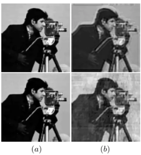
(a) K + s (b) K ∗ u (c) s ∗ u (d) (K + s) ∗ u Fig. 1. The influence of the noise s present in the blurring kernel. Top: Gaussian blur kernel K of support 11 × 11 with σb = 1 and s ∼ N (0, 72). Bottom: Gaussian blur
kernel K with support 71 × 71 with σb= 1 and s ∼ N (0, 0.82). PSNR: top (d) 20.0824,
bottom (d) 20.9103.
kernels (K +s) and extension to the multichannel (color) case and to static video restoration.
We first illustrate in Figure 1 this type of degradation on a real grey-scale image, in the case n = 0. We separate the degraded image f = (K + s) ∗ u shown in Fig. 1 (d) into two parts, K ∗ u and s ∗ u, and we visualize K ∗ u, s ∗ u in Fig. 1, to see how the noise s in the blurring kernel K influences the degraded image f . We use two blurring kernels (K + s) with different support sizes, which leads to different degrees of degradation, perturbations or severe noise, that can be seen by looking at s ∗ u in Fig. 1. We notice that much of the information is kept in the K ∗ u term; thus, we propose here to consider s ∗ u as noise also (dependent on the unknown image u). Therefore, we reformulate the degradation model as
f = K ∗ u + ns,u,n,
with a new noise term ns,u,n= s ∗ u + n. Because this reformulated degradation model looks like the standard one, we can attempt to apply the Rudin-Osher model [36] to recover u from f , as shown in Fig. 2 (b), and we compare these results with the case when s is known (Fig. 2 (a)). Of course, the recovery of u using the RO model, in the (nonrealistic) case when s is known, gives excellent results. However, as seen in Fig. 2 (b), the restored images using the RO model (1) with unknown s have visual artifacts and low PSNR, compared to the recovered images using the RO model with known s (replacing K by the true Ks= K + s in (1)). Thus, the results in Fig. 2 (b) with unknown s are not satisfactory. Moreover, the blind deconvolution methods [44, 10, 21, 29] within the variational framework cannot be applied directly, since they assume that the unknown blur kernel is sufficiently smooth or at least piecewise smooth, which
(a) (b)
Fig. 2. Recovered images from the degraded images in Fig. 1 (d) using (a) RO model with known s and one frame, using (b) RO model with unknown s and one frame. Top: recovery of Fig. 1 top (d). Bottom: recovery of Fig. 1 bottom (d). PSNR: top (a) 35.0097, (b) 23.0409, bottom (a) 36.5113, (b) 21.5140.
is not the case here. We conclude that it is very difficult to recover an image degraded by noisy blur kernel, as long as the noise s in the blurring kernel is unknown. For this reason, we make the problem slightly easier, by assuming that several frames (noisy-blurry versions of the same image u) are available, instead of only one, as presented next. The idea of using several degraded frames in the reconstruction of a single restored image is not new. Usually, low-resolution noisy-blurry frames are available to obtain a super-resolution image, as in [6], [33], [39, 32, 13], among other work. We mention that a preliminary version of this work has been presented at the International Conference in Image Processing ICIP 2009 [24].
2
Description of the proposed model
We borrow the idea of the multiframe model proposed for image super-resolution by Marquina-Osher [28]: we consider N given data frames (or a multiframe)
fk= (K + sk) ∗ u + nk,
with unknown noise terms sk, nk, k = 1, 2, ..., N of zero mean and variances σ2s and σ2
n, respectively (e.g., N available data captured by a static video camera under bad atmospheric conditions and distortions caused by high temperatures and air turbulence). Then, similarly, we reformulate the degradation model fk= (K + sk) ∗ u + nk as
with new unknown noise terms nsk,u,nk = sk ∗ u + nk, k = 1, 2, · · · , N . Hence,
we formulate the general minimization problem with the above reformulated degradation model incorporating a multiframe
min u (N X k=1 Φ(fk− K ∗ u) + Ψ (|∇u|) )
where Φ and Ψ define the fidelity and regularizing terms respectively. We will take advantage of the following known property [18], used here as follows: if we define at any point x
g = 1 N N X k=1 fk = K ∗ u + ³ 1 N N X k=1 sk ´ ∗ u +³ 1 N N X k=1 nk ´ ,
recalling that the noise terms sk and nkare of zero mean and uncorrelated with
u, then it follows that
E{g(x)} = K ∗ u(x),
where E{g(x)} is the expected value of g. The variance of g −K ∗u, σ2
g(x)−K∗u(x) at x is expressed as:
σ2
g(x)−K∗u(x)= E{(g(x) − K ∗ u(x))2} = E Ã ³ 1 N N X k=1 sk ´ ∗ u(x) +³ 1 N N X k=1 nk ´!2 = E Ã ³ 1 N N X k=1 sk ´ ∗ u(x) !2 + E ( ³ 1 N N X k=1 nk(x) ´2) = 1 Nσ 2 (s∗u)(x)+ 1 Nσ 2 n(x) where σ2
(s∗u)(x)and σn(x)2 are the variances at x of s ∗ u and n respectively. Thus, the standard deviation at any point of this residual is
σg(x)−K∗u(x)= 1 √ N q σ2 (s∗u)(x)+ σn(x)2 .
As N increases, the variability of the pixel values at each location x decreases. Because E{g(x)} = K ∗ u(x), this means that g(x) approaches K ∗ u(x) as the number of noisy images used in the averaging process increases.
Now we propose two multiframe minimization problems based on the general multiframe model for grey-scale image restoration.
2.1 Multiframe/RO model
Assuming given fk ∈ L2(Ω), k = 1, ..., N , we formulate a first minimization problem based on RO model [36],
min u ( E(u) = λ 2 Z Ω N X k=1 µk(fk− K ∗ u)2dx + Z Ω |∇u|dx ) , (2)
where λ > 0 and µk> 0 are given parameters with PN
k=1µk= 1. The associated Euler-Lagrange equation is given by
∂E ∂u = λ ( N X k=1 µkK ∗ (K ∗ u − f˜ k) ) − ∇ · µ ∇u |∇u| ¶ = 0,
which, due to the linearity of the blurring operator, is simplified to
∂E ∂u = λ n ˜ K ∗ (K ∗ u − f )o− ∇ · µ ∇u |∇u| ¶ = 0,
where ˜K(x) = K(−x) and f = PNk=1µkfk is the weighted average of fk’s. If we choose uniform weights µk = N1, then ¯f = g the arithmetic mean of fk’s. Following [28], we also consider different weights µk = PNT V (fk)
k=1T V (fk)
, thus we call
f the TV-mean of fk’s in this case. We note that the PSNR values (peak signal-to-noise ratio computed using the true image u) for f and for the arithmetic mean g = PNk=1 1
Nfk are larger than the PSNR for each fk. However, both TV-mean and arithmetic mean are still blurry versions of the unknown image u.
2.2 Multiframe/Nonlocal TV model
We formulate a second minimization problem based on nonlocal methods. Start-ing with Buades et al. [8], nonlocal patch based methods [12] have been explored in many papers in image denoising, including [25], [16], [17], because these are well adapted to texture denoising while the standard denoising models working with local image information seem to consider texture as noise, which results in losing details. We consider the nonlocal total variation regularization proposed by Gilboa-Osher [16], [17], instead of the local one, using the notions of non-local gradient and nonnon-local divergence inspired from graph-based methods [45]. Anisotropic smoothing is applied in both spatial and intensity neighborhoods [43].
Let u : Ω → R be a function, and w : Ω × Ω → R be a nonnegative and symmetric weight function. The nonlocal gradient vector ∇wu : Ω × Ω → R is (∇wu)(x, y) := (u(y) − u(x))
p
w(x, y). Hence, the norm of the nonlocal gradient
of u at x ∈ Ω is defined as
|∇wu|(x) := sZ
Ω
(u(y) − u(x))2w(x, y)dy.
The nonlocal divergence divw−→v : Ω → R of the vector −→v : Ω ×Ω → R is defined as the adjoint of the nonlocal gradient,
(divw−→v )(x) := Z
Ω
Based on these nonlocal operators, Gilboa-Osher proposed the nonlocal TV reg-ularizer (NLTV), Z Ω |∇wu|dx := Z Ω sZ Ω
(u(y) − u(x))2w(x, y)dydx,
which corresponds in the local case to T V (u) =RΩ|∇u|dx.
Now we similarly propose a minimization problem with the nonlocal TV regularizer and multiframe model
min u ( E(u) = λ 2 Z Ω N X k=1 µk(fk− K ∗ u)2dx + Z Ω |∇wu|dx ) , (3)
where λ > 0 and µk > 0 are given parameters with PN
k=1µk = 1. Similarly, we obtain the simplified Euler-Lagrange equation based only on the mean f ,
∂E ∂u = λ n ˜ K ∗ (K ∗ u − f ) o − ∇w· µ ∇wu |∇wu| ¶ = 0, where ∇w· µ ∇wu |∇wu| ¶ (x) = Z Ω (u(y) − u(x))w(x, y) · 1 |∇wu|(y) + 1 |∇wu|(x) ¸ dy.
Furthermore, in practice, we use the weight function w at (x, y) ∈ Ω × Ω depending on an image q : Ω → R, wq(x, y) = exp ³ −da(q(x), q(y)) h2 ´ , da(q(x), q(y)) = Z R2 Ga(t)|q(x + t) − q(y + t)|2dt,
where dais the patch distance, Gais the Gaussian kernel with standard deviation
a determining the patch size, and h is the filtering parameter which corresponds
to the noise level [8]. The weight function w(x, y) gives the similarity of the intensity values as well as of image features between two pixels x and y in the image q, which will be defined in Section 2.3. Note that, with a given noisy data (no blur), the weights w are usually computed from the data itself. Recently for image deblurring and denoising, Lou et al. [26] used a preprocessed image q to define the weights w, obtained by applying the Wiener filter to the blurry-noisy data. Also, in practice, for a fixed pixel x ∈ Ω, we use a search window
S(x) = {y ∈ Ω : |x − y| ≤ r} to compute w(x, y) instead of Ω.
2.3 Extension to multichannel data
Now we consider the multichannel (color) degradation models defined as (A) fi= (K + s) ∗ ui+ ni, i ∈ {r, g, b} or
(a) (b) (c) (d)
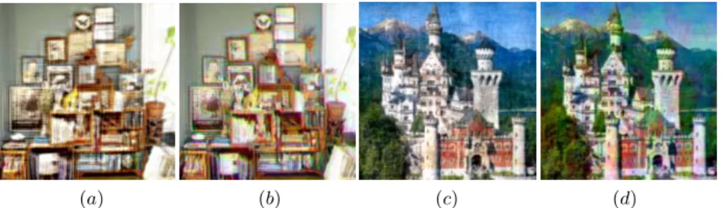
Fig. 3. Degraded images (K + s) ∗ u, (a)-(b): with Gaussian blur kernel K of support 22 × 22 with σb = 1, s ∼ N (0, 42), (c)-(d): with Gaussian blur kernel K of support
176 × 176 with σb = 1, s ∼ N (0, 0.42). (a), (c): type A (b), (d): type B. PSNR: (a)
16.8572, (b) 17.3500, (c) 18.0546, (d) 17.6463.
which are illustrated in Fig. 3 on real images, in the case ni = 0. We observe that even though the degraded images (a) and (b) (or (c) and (d)) by the above degradation models (A) and (B) respectively look different, the type of degra-dations are similar in the sense that the data (a) and (b) (or (c) and (d)) with a small size of blur kernel K (or a large size of K) produce perturbations (or severe noise) like in the grey-scale case. Thus, we again use the multiframe idea for the multichannel version.
Assuming N given data frames (a multiframe), we reformulate the degrada-tion models as
(A.2) fki = (K + sk) ∗ ui+ nik= K ∗ ui+ nisk,ui,nik, i ∈ {r, g, b}
(B.2) fki = (K + sik) ∗ ui+ nik= K ∗ ui+ nisi
k,ui,nik, i ∈ {r, g, b}
where sk (or sik) and nik, k = 1, 2, · · · , N , are unknown noise terms of zero mean and variances σ2
s and σ2n respectively, nisk,u,nk = sk∗ u
i+ ni
k, and nisi k,u,nk =
si
k ∗ ui+ nik. Hence, we end up with the same degradation models (A.2) and (B.2) considering both ni
sk,u,nk and n
i si
k,u,nk as noises, which leads to a similar
minimization problem: Multiframe/RO model min u E(u) = λ 2 Z Ω N X k=1 µk X i=r,g,b (fki − K ∗ ui)2 dx + Z Ω k∇ukdx , (4)
where λ > 0, µk > 0 are given parameters with PN k=1µk = 1, k∇uk is defined by k∇uk =s X i=r,g,b [(ui x)2+ (uiy)2],
andRΩk∇ukdx is a generalization of TV regularization to color images with
cou-pled channels [5, 7]. Using the linearity of K, we obtain the simplified associated Euler-Lagrange equations given by
∂E ∂ui = λ n ˜ K ∗ (K ∗ ui− fi)o− ∇ · µ ∇ui k∇uk ¶ = 0, i ∈ {r, g, b}
where fi = PNk=1µkfki is the weighted average of fki for each i ∈ {r, g, b} (i.e. f =R PNk=1µkfk is the weighted average of fk). Note that we use µk =
Ωk∇fkkdx
PN k=1
R
Ωk∇fkkdx
corresponding to the TV-mean in Section 2.1. Moreover, ¯f is
still a blurry version of the ideal color image u.
Similarly, we also formulate the color version of Multiframe/Nonlocal TV model by extending the scalar nonlocal operators to the vector-valued ones: Multiframe/Nonlocal TV model min u E(u) = λ 2 Z Ω N X k=1 µk X i=r,g,b (fi k− K ∗ ui)2 dx + Z Ω k∇wukdx , (5)
where λ > 0, µk > 0 are given parameters with PN k=1µk= 1, and k∇wuk : Ω → R is defined as k∇wuk(x) := s X i=r,g,b |∇ui w|2(x) := s X i=r,g,b Z Ω (ui(y) − ui(x))2w(x, y)dy
with the weight function w = wq : Ω × Ω → R defined in Section 2.2, computed by the following patch distance
da(q(x), q(y)) = Z
R2
Ga(t)kq(x + t) − q(y + t)k2dt.
The Euler-Lagrange equations are also given based only on the means fi by
∂E ∂ui = λ n ˜ K ∗ (K ∗ ui− fi) o − ∇w· µ ∇wui k∇wuk ¶ = 0, i ∈ {r, g, b} where ∇w· µ ∇wui k∇wuk ¶ (x) = Z Ω (ui(y) − ui(x))w(x, y) · 1 k∇wuk(y) + 1 k∇wuk(x) ¸ dy.
We define now q, to be used in the computation of weights w. First, we simply use the mean ¯f as q because even though ¯f ≈ K ∗ u is a blurry image, it still
can keep well the geometrical configurations of the original image u. Second, we use another image, a sharper image ¯g, instead of ¯f :
¯
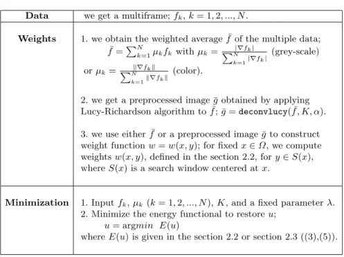
Table 1. Algorithm of Multiframe/NLTV Model Data we get a multiframe; fk, k = 1, 2, ..., N .
Weights 1. we obtain the weighted average ¯f of the multiple data;
¯ f =PNk=1µkfk with µk= PN|∇fk| k=1|∇fk| (grey-scale) or µk=PNk∇fkk k=1k∇fkk (color).
2. we get a preprocessed image ¯g obtained by applying
Lucy-Richardson algorithm to ¯f ; ¯g = deconvlucy( ¯f , K, α).
3. we use either ¯f or a preprocessed image ¯g to construct
weight function w = w(x, y); for fixed x ∈ Ω, we compute weights w(x, y), defined in the section 2.2, for y ∈ S(x), where S(x) is a search window centered at x.
Minimization 1. Input fk, µk (k = 1, 2, ..., N ), K, and a fixed parameter λ.
2. Minimize the energy functional to restore u;
u = argmin E(u)
where E(u) is given in the section 2.2 or section 2.3 ((3),(5)).
where deconvlucy is Lucy-Richardson deconvolution method [27, 34], an itera-tive procedure for recovering an ideal image from the blurred image ¯f with a
known point spread function K, and α is the number of iterations the deconvlucy function performs. Note that we in practice generate a data using imfilter in MATLAB:
either (1) fk= imfilter(u, K + sk,0circular0,0conv0), k = 1, 2, ..., N or (2) fk= imfilter(u, K + sk,0symmetric0,0conv0), k = 1, 2, ..., N .
Here, for the second case (2), if we apply imfilter directly to ¯f , then the
gener-ated image ¯g has some artifacts near the boundary that look like ringing effect.
To avoid this, we first expand the mean ¯f to ˆ¯f such as ˆ¯f = padarray( ¯f , [m m],0symmetric0) and we apply deconvlucy to ˆ¯f producing ˆ¯g, and then reduce ˆ¯g again to the original size, which provides a preprocessed image ¯g for the data
(2). We used m = 10, and for the first case (1), we apply deconvlucy directly to the ¯f . In practice, we use q = ¯f for grey-scale images, and q = ¯f or q = ¯g for
color images, so we compare the recovered images with q = ¯f or q = ¯g.
2.4 Application to joint restoration and binary segmentation
Here we present another application of the multiframe idea, joint segmenta-tion and restorasegmenta-tion of a binary image degraded by a noisy blur kernel, from several frames. First, let φ : Ω → R be a level set function (usually a Lip-schitz continuous function) whose zero level set represents the evolving curve
C = {x ∈ Ω : φ(x) = 0} [31], [37], and define f : Ω → R by the given data to be
restored and segmented, assuming the degradation
f = (K + s) ∗ u + n = (K + s) ∗ ³ c1H(φ) + c2(1 − H(φ)) ´ + n,
which is an extension of the degradation model f = K ∗ ³
c1H(φ) + c2(1 −
H(φ))´+ n proposed in [23] for joint denoising, deblurring and segmentation of a binary image u, with unknown constants c1, c2, and one-dimensional Heaviside
function H.
Again, assuming N given data frames, we formulate the binary image seg-mentation and restoration minimization problem incorporating a multiframe:
min c1,c2,φ n E(c1, c2, φ) = 1 2 Z Ω ³XN l=1 µl ¯ ¯ ¯fl− K ∗ ³ c1H(φ) + c2(1 − H(φ)) ´¯¯ ¯2 ´ dx +λ Z Ω |∇H(φ)|dxo, (6)
where λ > 0, µl> 0 are given parameters with PN
l=1µl= 1.
We compute the Euler-Lagrange equations minimizing the energy E with respect to c1, c2, and φ. Using alternating minimization, keeping first φ fixed
and minimizing the energy with respect to the unknown constants c1 and c2, we
obtain the following linear system of equations:
c1 Z Ω k2 1dx + c2 Z Ω k1k2dx = Z ¯ f k1dx, c1 Z Ω k1k2dx + c2 Z Ω k2 2dx = Z ¯ f k2dx
with the mean ¯f =PNl=1µlfl, k1= K ∗ H(φ) and k2 = K ∗ (1 − H(φ)). Note
that the linear system has a unique solution because the determinant of the coefficient matrix is not zero due to the Cauchy-Schwartz inequality [23].
Keeping now the constants c1 and c2 fixed and minimizing the energy with
respect to φ, we obtain the simplified Euler-Lagrange equation involving only the mean ¯f of given multiple frames
∂E ∂φ = δ(φ) h ³ ˜ K ∗ ¯f − c1K ∗ (K ∗ H(φ)) − c˜ 2K ∗ (K ∗ (1 − H(φ)))˜ ´ · (c2− c1) − µ∇ ·³ ∇φ |∇φ| ´i = 0,
where δ denotes the one-dimensional Dirac distribution (in practice, we substi-tute H and δ by smooth approximations, as in [9]).
2.5 Numerical approximations
Minimization of the proposed energy functionals E(u) (or E(c1, c2, φ) with fixed
c1, c2 from Section 2.4) is carried out using the Euler-Lagrange equations with
homogeneous Neumann boundary conditions ∂u/∂n = 0 (or ∂φ/∂n = 0), where
n is the exterior normal to the image boundary. We already presented the
Euler-Lagrange equations ∂E(u)/∂u = 0 and ∂E(c1, c2, φ)/∂φ = 0 of the models
(2)-(5) and (6) respectively, in the previous sections. Based on these Euler-Lagrange equations, we use the steepest gradient descent scheme,
∂u ∂t = − ∂E(u) ∂u , or ∂φ ∂t = − ∂E(c1, c2, φ) ∂φ .
The basic discretizations are presented next, separating the local and nonlocal cases.
Multiframe/RO or Multiframe Segmentation model Let uσ
i,j denote the discretized version of uσ(x, y) with (x, y) ∈ Ω in channel σ; σ ∈ {r, g, b} for the multichannel case, but for the grey-scale case we replace uσby u. The forward and backward finite difference approximations of the derivatives ∂uσ
i,j/∂x and
∂uσ
i,j/∂y are respectively defined by
∆x
±uσi,j = ±(uσi±1,j− uσi,j), ∆y±uσi,j= ±(uσi,j±1− uσi,j), and the central finite difference approximation is
∆x cuσi,j= uσ i+1,j− uσi−1,j 2 , ∆ x cuσi,j= uσ i,j+1− uσi,j−1 2 .
The discretization of k∇uk2was carried out using the central difference scheme
k∇uk2= X
σ∈{r,g,b} (∆x
cuσi,j)2+ (∆xcuσi,j)2.
Terms of the form ∇ · (c(x, y)∇uσ) were discretized using forward difference for the gradient and backward difference for the divergence
∇ · (c(x, y)∇uσ) = ∆x
−(c(i, j)∆x+uσi,j) + ∆y−(c(i, j)∆y+uσi,j). Multiframe/NLTV model Let uσ
k denote the value of a pixel k in the image (1 ≤ k ≤ N ) with channel σ (i.e. the discretized version of uσ(x) defined on Ω), and let pσ
k,l be the discretized version of pσ(x, y) with x, y ∈ Ω. wk,l is the sparsely discrete version of w = w(x, y) : Ω × Ω → R. We use the neighbors set l ∈ Nk defined as l ∈ Nk := {l : wk,l> 0}. Then we have ∇wd and divwd, the discretizations of ∇wand divw, defined respectively as [17]
∇wd(uσk) := (uσl − uσk) √ wk,l, l ∈ Nk, divwd(pσk,l) := X l∈Nk (pσ k,l− pσl,k) √ wk,l.
Moreover, the magnitude of pσ
k,l at k is |pσ|k = qP
l(pσk,l)2, thus the discretiza-tion of k∇uwk2(x) was done as
k∇uwdk2k= X σ∈{r,g,b} |∇wduσ|2k = X σ∈{r,g,b} X l (uσ l − uσk)2wk,l.
We construct the weight function wk,l, following the algorithm in [16]: for each pixel k, (1) take a patch Bk around a pixel k, compute the distances (da)k,l (a discretization of da) to all the patches Bl in the search window l ∈ S(k), and construct the neighbors set Nk by taking the m most similar and the four nearest neighbors of the pixel k, (2) compute the weights wk,l defined in Section 2.2, l ∈ Nk and set to zero all other connections (wk,l = 0, l /∈ Nk), (3) set
wk,l= wl,k, l ∈ Nk. In all the examples, we used m = 5, so a maximum of up to 2m + 4 neighbors for each pixel is allowed in our implementation, and we used 5 × 5 pixel patches with a = 1, a search window of size 11 × 11. The complexity of computing the weights using this algorithm is N × W indowsize× (P atchsize×
Channalsize+logm). Thus, in our color case, we need 121×(25×3+2.5) ≈ 9619 operations per pixel. Most of the computation time is in this part.
3
Experimental results
We first test the proposed models (2)-(5) based on the multiframe approach, for the recovery of grey-scale and color images degraded by noisy blur kernel, using mostly 10 data frames (e.g. Fig. 4-14). We test on grey-scale images in Figures 4-7, and on color images in Figures 8-15, 17. As mentioned in Section 2.3, for Multiframe/NLTV model, we use the mean q = ¯f in the grey-scale case, and
a preprocessed image q = ¯g or q = ¯f in the color one to compute the weight
function w = wq. In Figures 11-14, we compared the recovered images using Multiframe/NLTV model (5) with different weight function w = wq; q = ¯g = deconvlucy( ¯f , α) by varying α or q = ¯f . In Fig. 15, with different number of
data frames k, we present the PSNR values of ¯f , the recovered images using the
proposed multiframe models (4), (5) vs k. In Fig. 17, we test on a real color video, each frame being degraded by varying noisy blur kernels (i.e. K + sk). At last, in Fig. 16, we test the proposed multiframe segmentation model (6) on severely degraded data.
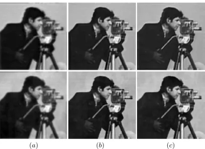
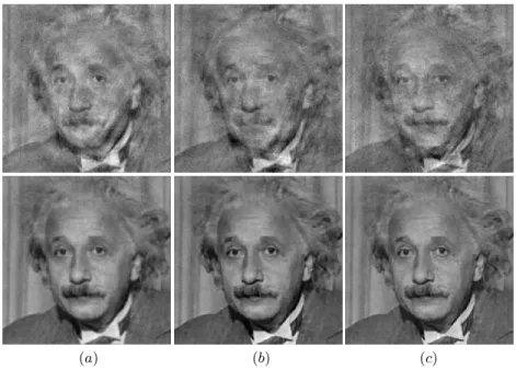
In Fig. 4, we recover the two different degraded image types shown in Fig. 1 (d), having some perturbations or severe noise induced by the noise sk in the blur kernel, using the proposed multiframe models (2), (3) with 10 frames. First, as expected, we observe that both models provide visually more satisfactory results than the one-frame RO model (1) (see Fig. 2 (b)), and much higher PSNR values. Moreover, Multiframe/NLTV model reduces the staircase effect appeared in the images recovered with Multiframe/RO model, and also gives higher PSNR values.
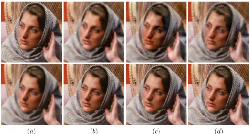
Similarly, in the case of the Barbara image in Fig. 5, containing texture, we can see that Multiframe/NLTV model produces again better recovered image,
especially by restoring well the texture, leading to higher PSNR than Multi-frame/RO model. We also compare the results with the one-frame RO model (1) and the proposed multiframe models. Even though the degradation in f does not look severe, one frame model (1) suffers from recovering the image, still keeping some artifacts (e.g. on the lower part of the face) generated by the noise
s. However, using the average of 10 noisy-blurry frames reduces very much the
perturbations, and produces much better recovered images with the proposed multiframe models.
In Figures 6 and 7, we use the pill box kernel with the same radius r = 2 but K + s of different supports, 31 × 31 in Fig. 6 and 71 × 71 in Fig. 7. As we have seen in the previous examples, the degraded image f = (K + s) ∗ u + n in Fig. 6 (one of the frames) corresponding to the small size of blurring kernel still has severe perturbations generated by the noise s, but the TV-mean f reduces the perturbations a lot, which leads to satisfactory recovered images. Similarly, the image f = (K + s) ∗ u + n in Fig. 7 corresponding to the large size of blur kernel seems to have severe noise, that is also generated by the noise s, but the average f reduces the noise leading to much higher PSNR, which results in a nice recovery of images.
In Figures 8-10, we recover the degraded color images by adding noise to the images (a)-(d), shown in Fig. 3 using imfilter function in MATLAB with Gaus-sian noise density d. First, as in the grey-scale case, we observe that the mean ¯f
reduces the perturbations or noise produced by the noise s ∗ u a lot, improving both visual quality and PSNR, which also leads to good recovered images in both models (4), (5). In all examples, Multiframe/NLTV model provides larger PSNR than Multiframe/RO model even though both produce visually very sim-ilar results. But in the case of the Barbara image in Fig. 13, containing texture, Multiframe/NLTV model gives better visual quality and larger PSNR, by re-covering texture better and with less artifacts on the face and hand. Moreover, despite some artifacts due to s ∗ u in the deblurred image ¯g (for example, ¯g in
Fig. 8 includes some amplification of the perturbations induced by s ∗ u), the recovered image using Multiframe/NLTV model with q = ¯g doesn’t include the
artifacts, producing cleaner image.
In Figures 11-14, we compare the recovered images using Multiframe/NLTV model (5) with the weights w = wq based on different q. In Fig. 11, we recovered the degraded images in Fig. 10 with q = ¯g by varying α. As seen both in Fig.
11 and in Fig. 12, as α increases, ¯g gets sharper, thus the PSNR value of the
recovered image increases, with the same optimal λ. Note that each example through Figures 8-12 has the same optimal λ; λ = 0.7 for Books and 0.6 for Castle in Fig. 8-9, λ = 0.7 for Books and 0.55 for Castle in Figures 10-12 regardless of q. Moreover, we also present the PSNR value of the recovered image with blurrier q = ¯f , resulting in smallest PSNR value. However, we cannot pursue a
high value of α all the time, since if ¯g has strong artifacts, the recovered image
also tends to keep these artifacts; in Fig. 14, the recovered images with q = ¯g, α = 10, give higher PSNR as well as better visual quality than the one with
with q = ¯f can provide even better visual quality than the one with q = ¯g; in
Fig. 14, the recovered image with q = ¯f gives the best visual quality, providing
clearer texture (left bottom part) and less artifacts near mouth, even though the PSNR value is slightly smaller.
In Fig. 15, we test the models with different number of frames k = 1, 3, 5, 7, 10, 15, 20, 25, 30 using the degraded images from Fig. 13. In all the cases, we fix the parameters λ = 10 for Multiframe/RO model (4), and λ = 12 for Multiframe/NLTV model (5). First, we observe that the PSNR values of ¯f seem
to increase slightly as k increases (despite of an exception at k = 25), while the ones of the recovered images using both multiframe models increase with large amount, especially until k = 7. This means that even slight change of ¯f induces
big improvement of the recovered image. Additionally, we present the recovered image using Multiframe/NLTV model from 30 frames, with much less artifacts both near the mouth and on the hand, and very well recovered texture part.
Furthermore, in Fig. 17, we present recovery of real color videos (fps=25) degraded by varying noisy blur kernels of type A or type B. We generate data using the pill-box kernel K of support 21×21 with radius r = 1.5, sk∼ N (0, 62), and nk with noise density d = 0.002. We use 25 data frames for ¯f , and we present the results of Lucy-Richardson method with ¯f , Multiframe/RO model,
and Multiframe/NLTV model with q = ¯f . Both multiframe models provide
cleaner images and higher PSNR values than Lucy-Richardson method, and again Multiframe/NLTV model gives better results by providing cleaner image, especially edge parts, and higher PSNR than Multiframe/RO model. Addition-ally, we present the PSNR values of ¯f , ¯g, recovered images using Multiframe/RO
and Multiframe/NLTV model, at every second, i.e. using 25 frames per second. Note that the videos can be found on the website: http://www.math.ucla.edu/
∼gomtaeng/research.html.
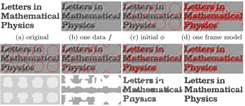
Lastly, Fig. 16 shows a successful segmentation and restoration from a severely degraded image by a noisy blur kernel. As seen in (d) in the top row, one frame method fails to find the object boundary. But, the proposed multiframe model (6) gives smooth curve evolution, leading to successful object detection as well as good restoration of image u, which can be seen in the middle and bottom rows. Here we generate 25 data frames using Gaussian kernel K of support 22 × 22 with σb= 1, sk ∼ N (0, 102), and nk∼ N (0, 102).
For the computational time, e.g., in Multiframe/NLTV model with the mul-tichannel case, it takes about 5 minutes for constructing the weight function of a 256 × 256 color image with the 11 × 11 search window and 5 × 5 patch in MATLAB on a dual core laptop with 2GHz processor and 2GB memory. Once we have constructed the weight, the minimization for u based on the gradient descent method takes about 50 seconds to compute 500 iterations.
4
Summary and Conclusions
We introduced a new degradation model with a noisy blur kernel, providing two different types of degradations such as perturbations or severe noise. We consider
the image restoration problem within the variational framework, by formulating the minimization problems called Multiframe/RO and Multiframe/NLTV; we assume that multiple noisy-blurry data are given with the same noise variance for the noise in the blur kernel. Both models give satisfactory results visually as well as according to PSNR. In addition, Multiframe/NLTV model incorporating nonlocal regularizer, well-known for texture denoising, provides better results than Multiframe/RO model. However, we also have a limitation, in the sense that we need more than one frame to ensure satisfactory recovery. As seen in Fig. 2, we would obtain very good results from one frame when s is known. Applications to color images, real videos, and binary image segmentation are also illustrated.
References
1. M.R. Bhatt, U.B. Desai, “Robust Image Restoration Algorithm Using Markov Ran-dom Field Model”, CVGIP: Graphical Models and Image Processing 56(1): 61-74, 1994.
2. M. Bilgen, H.S. Hung, “Restoration of noisy images blurred by a random point spread function”, IEEE Int. Symp. on Circuits and Systems 1: 759-762, 1990. 3. M. Bilgen, W.H. Brockman, “Restoration of noisy images blurred by a random
medium”, 1992.
4. M. Bilgen, H.S. Hung, “Constrained least-squares filtering for noisy images blurred by random point spread function”, Opt. Eng. 33(6): 2020-2023, 1994.
5. P. Blomgren, T.F. Chan, “Color TV: Total variation methods for restoration of vector-valued images”, IEEE TIP 7(3): 304-309, 1998.
6. N.K. Bose, M.K. Ng, A.C. Yau, “A fast algorithm for image super-resolution from blurred observations”, EURASIP J. Applied Sign. Proc. 1-14, 2006.
7. A. Brook, R. Kimmel, N. Sochen,“Variational restoration and edge detection for color images”, J. Math. Imag. Vis., vol. 18, pp. 247268, 2003.
8. A. Buades, B. Coll, J.M. Morel, “A review of image denoising algorithms, with a new one”, SIAM MMS 4(2): 490-530, 2005.
9. T.F. Chan, L.A. Vese, “Active contours without edges”, IEEE TIP 10(2): 266-177, 2001.
10. T.F. Chan, C.K. Wong, “ Total variation blind deconvolution”, IEEE TIP 7(3): 370-375, 1998.
11. P.L. Combettes, H.J. Trussell, “Methods for Digital Restoration of Signals De-graded by a Stochastic Impulse Response”, IEEE Trans. Acoustics, Speech and Signal Processing 37: 393-401, 1989.
12. A. Efros, T. Leung, “Texture synthesis by non-parametric sampling”, ICCV, 1999. 13. S. Farsiu, D. Robinson, M. Elad, P. Milanfar, “Fast and Robust Multi-frame
Super-resolution”, IEEE TIP 13(10): 1327-1344, 2004.
14. S. Geman, D. Geman, “ Stochastic relaxation, Gibbs distributions, and the Bayesian restoration of images”, IEEE TPAMI 6: 721-741, 1984.
15. D. Geman, G. Reynolds, “Constrained Restoration and the Recovery of Disconti-nuities”, IEEE T on PAMI, Vol. 14, No. 3, 1992.
16. G. Gilboa, S. Osher, “Nonlocal linear image regularization and supervised segmen-tation”, SIAM MMS 6(2): 595-630, 2007.
17. G. Gilboa, S. Osher, “Nonlocal operators with applications to image processing”, SIAM MMS 7(3): 1005-1028, 2008.
(a) (b) (c)
Fig. 4. TV-mean ¯f and recovered images with multiframe models. Top: (a) ¯f from
10 data frames with one frame shown in Fig. 1 top (d); recovered images using (b) Multiframe/RO, (c) Multiframe/NLTV. Bottom: (a) ¯f from 10 data frames with one
frame shown in Fig. 1 bottom (d); recovered images using (b) Multiframe/RO, (c) Mul-tiframe/NLTV. PSNR: top (a) 22.4973, (b) 26.8390, (c) 27.1252, bottom (a) 22.6994, (b) 26.8036, (c) 27.1490.
(a) (b) (c)
Fig. 5. Recovered images with multiframe models. Top: (a) original image, (b) de-graded image (one frame) f = (K + s) ∗ u with the given K + s in bottom (a) in Fig. 1, (c) recovered image using RO model with the unknown s and one frame. Bottom: (a) f from 10 data frames, recovered images using (b) Multiframe/RO, (c) Multi-frame/NLTV. PSNR: top (b) 22.1770, (c) 22.8667, bottom (a) ¯f : 22.9172, (b) 24.2993,
(a) (b) (c)
Fig. 6. Top: degraded images fk= (K +sk)∗u+nk, k = 1, 2, 3 (out of 10 data frames),
with the pill-box kernel K of support 31 × 31 and radius r = 2, sk ∼ N (0, 52) and nk∼ N (0, 52). Bottom: (a) f =P10
k=1µkfk from the top row, recovered images using
(b) Multiframe/RO, (c) Multiframe/NLTV. PSNR: top (a) 20.2258, (b) 17.5298, (c) 21.2778, bottom (a) ¯f : 25.4886, (b) 28.3715, (c) 28.9649.
(a) (b) (c)
Fig. 7. Top: degraded images fk= (K +sk)∗u+nk, k = 1, 2, 3 (out of 10 data frames),
with the pill-box kernel K of support 71 × 71 and radius r = 2, sk ∼ N (0, 22) and nk∼ N (0, 102). Bottom: (a) f =P10
k=1µkfkfrom the top row, recovered images using
(b) Multiframe/RO, (c) Multiframe/NLTV. PSNR: top (a) 21.4679, (b) 21.3775, (c) 22.4948, bottom (a) f : 28.3977, (b) 30.7696, (c) 31.1031.
(a) (b) (c)
Fig. 8. (A) Top: (a) original image, (b) degraded image (one frame) f = (K + s) ∗ u + n with the same (K + s) in Fig. 3 (a) and noise density d = 0.001, (c) f from 10 data frames. Bottom: (a) ¯g with α = 15, recovered images using (b) Multiframe/RO, (c)
Multiframe/NLTV with q = ¯g. PSNR: top (b) f : 16.1659, (c) f : 18.6177, bottom (a)
21.0103, (b) 20.5248, (c) 20.8851.
(a) (b) (c)
Fig. 9. (A) Top: (a) original image, (b) degraded image (one frame) f = (K + s) ∗ u + n with the same (K + s) in Fig. 3 (c) and noise density d = 0.005, (c) f from 10 data frames. Bottom: (a) ¯g with α = 15, recovered images using (b) Multiframe/RO, (c)
Multiframe/NLTV with q = ¯g. PSNR: top (b) f : 17.0298, (c) f : 19.5645, bottom (a)
(a) (b) (c) (d)
Fig. 10. (B) (a) degraded image (one frame) f = (K + s) ∗ u + n (top) with the same (K + s) in Fig. 3 (b) and noise density d = 0.001, (bottom) with the same (K + s) in Fig. 3 (d) and noise density d = 0.005, (b) f from 10 data frames, recovered images using (c) Multiframe/RO, (d) Multiframe/NLTV with q = ¯g and α = 15. PSNR: top
(a) 17.1705, (b) ¯f : 18.7907, (c) 20.4440, (d) 20.5432, bottom (a) 16.7133, (b) ¯f : 19.5224,
(c) 20.9269, (d) 21.2115.
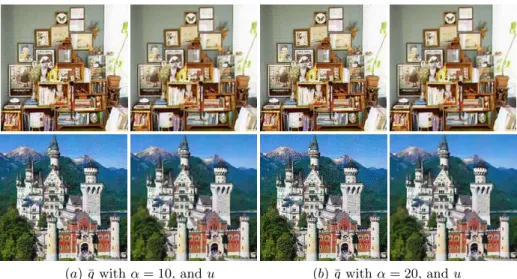
(a) ¯g with α = 10, and u (b) ¯g with α = 20, and u
Fig. 11. Recovered images u using Multiframe/NLTV with different α for q = ¯g with
the given data (a) in Fig. 10. 1st, 3rd column: ¯g with α = 10 and α = 20 respectively.
Recovered image u with different weight function wq (same optimal λ)
q g with α = 7¯ α = 10 α = 15 α = 20 mean ¯f
Books (B) PSNR(u)= 20.3648 20.4544 20.5432 20.5727 20.2725 Castle (B) PSNR(u)= 21.0196 21.1282 21.2115 21.2192 20.8830
Fig. 12. Comparison of the recovered image u from the degraded images (a) in Fig. 10 using Multiframe/NLTV with different weight function wq. λ = 0.7 for Books, 0.55 for
Castle.
(a) (b) (c) (d)
Fig. 13. (A) Top: (a) original image, (b)-(d) degraded images fk = (K + sk) ∗ u, k = 1, 2, 3 (out of 10 data frames), with the pill-box kernel K of support 71 × 71 and
radius r = 2.5, sk ∼ N (0, 0.82). Bottom: (a) f from 10 data frames, (b) recovered
image using Multiframe/RO, (c) ¯g with α = 10, (d) ¯g with α = 20. PSNR: top (b)
21.4318, (c) 20.9718, (d) 21.1142, bottom (a) ¯f : 22.1743, (b) 26.5147, (c) 24.9449, (d)
26.2488.
(a) (b) (c)
Fig. 14. Recovered images using Multiframe/NLTV with (a) q = ¯f , (b) q = ¯g with α = 10, (c) q = ¯g with α = 20 in Fig. 13. PSNR: (a) 27.1031 (λ = 11), (b) 27.1758
Fig. 15. Graph of PSNR versus the number of frames k used (using the degraded images in Fig. 13). (a) PSNR values of ¯f , recovered image using Multiframe/RO (fixed λ = 10), Multiframe/NLTV with q = ¯f (fixed λ = 12) vs k, (b) recovered image using
Multiframe/NLTV with k = 30 with optimal λ = 20: PSNR=29.1959.
(a) original (b) one data f (c) initial φ (d) one frame model
Fig. 16. Segmentation of a binary image degraded by a noisy blur kernel. Top: (d) final curve (zero level set of φ) with one data f . Middle, Bottom: segmentation using 25 data frames, curve evolution (middle), and the corresponding recovered images u =
Type.A.
Type.B.
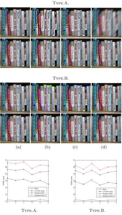
(a) (b) (c) (d)
Type.A. Type.B.
Fig. 17. Real video restoration of type A (1st, 2nd row) and B (3rd, 4th row). Top (1st, 3rd row): (a) one original sequence, (b)-(d) degraded sequences (out of 25 data frames). Bottom (2nd, 4th row): (a) ¯f =P25k=1from the corresponding top row, (b) ¯g
with α = 10, recovered image using (c) Multiframe/RO and (d) Multiframe/NLTV with
q = ¯f . 5th row: plots of PSNR values of ¯f , ¯g, recovered images using Multiframe/RO
and Multiframe/NLTV model, at every second, i.e. using 25 frames per second. PSNR of type A: top (b) 17.3221, (c) 16.5711, (d) 18.0077, bottom (a) ¯f : 21.1275, (b) 24.2129,
(c) 25.6732, (d) 26.7694. PSNR of type B: top (b) 16.8509, (c) 17.1406, (d) 17.0949, bottom (a) ¯f : 21.2134, (b) 24.1186, (c) 25.5584 , (d) 26.5092. Note that videos are
18. R.C. Gonzalez, R.E. Woods, “Digital Image Processing”, 3rd edition, Prentice-Hall, 2008.
19. L. Guan, R.K. Ward, “Restoration of stochastically blurred images by the geomet-rical mean filter”, Opt. Eng. 29, 289-295, 1990.
20. M.L. Hambaba, “Robust deblurring of random blur”, Applied Optics, 33(14): 2877-2882, 1994.
21. L. He, A. Marquina, S.J. Osher, “Blind deconvolution using TV regularization and Bregman iteration”, Int. J. Imaging Syst. Technol., Vol. 15, pp. 74-83, 2005. 22. B.R. Hunt, “The application of constrained least squares estimation to image
restoration by digital computer”, IEEE Trans. Comput. 22, 805812, 1973.
23. M. Jung, G. Chung, G. Sundaramoorthi, L.A. Vese, A.L. Yuille, “Sobolev gra-dients and joint variational image segmentation, denoising and deblurring”, SPIE proceedings on Electronic Imaging, 2009.
24. M. Jung, A. Marquina, L.A. Vese, “Multiframe Image Restoration in the Presence of Noisy Blur Kernel”, to appear, ICIP 2009.
25. S. Kindermann, S. Osher, P.W. Jones, “Deblurring and denoising of images by nonlocal functionals”, SIAM MMS 4(4): 1091-1115, 2005.
26. Y. Lou, X.Zhang, S. Osher, A. Bertozzi, “Image recovery via nonlocal operators”, Journal of Scientific Computing (to appear), 2009.
27. L.B. Lucy, “An iterative technique for the rectification of observed distributions”, Astronomical Journal 79(6): 745-754, 1974.
28. A. Marquina, S. Osher, “Image Super-Resolution by TV-Regularization and Breg-man Iteration”, JSC 37(3): 367-382, 2008.
29. A. Marquina, “Nonlinear Inverse Scale Space Methods for Total Variation Blind Deconvolution”, SIAM J. on Imaging Sci., vol. 2, pp. 64-83, 2009.
30. V.Z. Mesarovic, N.P. Galatsanos, A.K. Katsaggelos, “Regularized constrained total least-squares image restoration”, IEEE TIP 4(8): 1096-1108, 1995.
31. S. Osher, R. Fedkiw, “Level set methods and dynamic implicit surfaces”, Springer, New York, 2003.
32. M. Protter, M. Elad, H. Takeda, P. Milanfar, “Generalizing the Non-Local-Means to Super-resolution Reconstruction”, IEEE TIP 18(1): 36-51 , 2009.
33. D. Rajan, S. Chaudhuri, “Simultaneous estimation of super-resolved scene and depth map from low resolution defocused observations”, IEEE TPAMI 25(9): 1102-1117, 2003.
34. W. H. Richardson, “Bayesian-Based Iterative Method of Image Restoration”, JOSA 62 (1): 55-59, 1972.
35. L. Rudin, S. Osher, E. Fatemi, “Nonlinear Total Variation Based Noise Removal Algorithms”, Physica D 60: 259-268, 1992.
36. L. Rudin, S. Osher, “Total variation based image restoration with free local con-straints”, IEEE ICIP, vol. I, 1994. Austin, TX.
37. J.A. Sethian, “Level Set Methods and Fast Marching Methods Evolving Interfaces in Computational Geometry, Fluid Mechanics, Computer Vision, and Materials Sci-ence”, Cambridge University Press, 1999.
38. D. Slepian, “Linear least squares filtering of distorted images”, J. Opt. Soc. Am. 57, 918-922, 1967.
39. H. Takeda, P. Milanfar, M. Protter, M. Elad, “Superresolution Without Explicit Subpixel Motion Estimation”, IEEE TIP 18(9): 1958-1975, 2009.
40. R.K. Ward, B.E.A. Saleh, “Restoration of images distorted by systems of random impulse response”, J. Opt. Soc. Am. A 2(8): 1254-1259, 1985.
41. R.K. Ward, B.E.A. Saleh, “Restoration of images distorted by systems of random time-varying impulse response”, J. Opt. Soc. Am. A3, 800807, 1986.
42. R.K. Ward, B.E.A. Saleh, “Deblurring random blur”, IEEE Trans. Acoust. Speech Sig. Proc. ASSP-34, 14941498, 1987.
43. L.P. Yaroslavsky, Digital image processing: An Introduction. Springer, 1985. 44. Y. You, M. Kaveh, “Blind image restoration by anisotropic regularization”, IEEE
Transactions on Image Processing 8:3 pp. 396-407, 1999.
45. D. Zhou, B. Scholkopf, “A Regularization Framework for Learning from Graph Data”, In: Workshop on Statistical Relational Learning and Its Connections to Other Fields, 2004.