HAL Id: tel-01531784
https://pastel.archives-ouvertes.fr/tel-01531784
Submitted on 1 Jun 2017HAL is a multi-disciplinary open access archive for the deposit and dissemination of sci-entific research documents, whether they are pub-lished or not. The documents may come from
L’archive ouverte pluridisciplinaire HAL, est destinée au dépôt et à la diffusion de documents scientifiques de niveau recherche, publiés ou non, émanant des établissements d’enseignement et de
Direct Numerical Simulation of bubbles with Adaptive
Mesh Refinement with Distributed Algorithms
Arthur Talpaert
To cite this version:
Arthur Talpaert. Direct Numerical Simulation of bubbles with Adaptive Mesh Refinement with Dis-tributed Algorithms. Numerical Analysis [math.NA]. Université Paris Saclay (COmUE), 2017. En-glish. �NNT : 2017SACLX016�. �tel-01531784�
NNT : 2017SACLX016
1
Th`
ese de doctorat
de l’Universit´
e Paris-Saclay
pr´
epar´
ee `
a l’ ´
Ecole polytechnique
´
Ecole doctorale n
o573
Interfaces
Sp´ecialit´e de doctorat : Math´ematiques appliqu´ees
par
M. Arthur Talpaert
Simulation num´erique directe de bulles
sur maillage adaptatif avec algorithmes distribu´es
Th`ese pr´esent´ee et soutenue `a l’INSTN de Saclay, le 24 f´evrier 2017. Composition du Jury :
M. Nicolas Seguin Professeur (Pr´esident du jury)
Universit´e de Rennes 1
M. Tony Leli`evre Professeur (Rapporteur)
´
Ecole des Ponts ParisTech
M. Fr´ed´eric Lagouti`ere Professeur (Rapporteur)
Universit´e Claude Bernard Lyon 1
M. Gr´egoire Allaire Professeur (Directeur)
´
Ecole polytechnique
M. St´ephane Dellacherie Ing´enieur (Co-directeur)
Hydro-Qu´ebec
M. Bruno Despr´es Professeur (Examinateur)
Universit´e Paris 6
M. Yohan Penel Chercheur (Examinateur)
CEREMA
Abstract
This PhD work presents the implementation of the simulation of two-phase flows in condi-tions of water-cooled nuclear reactors, at the scale of individual bubbles. To achieve that, we study several models for Thermal-Hydraulic flows and we focus on a technique for the capture of the thin interface between liquid and vapour phases. We thus review some possible techniques for Adaptive Mesh Refinement (AMR) and provide algorithmic and computational tools adapted to patch-based AMR, which aim is to locally improve the precision in regions of interest. More precisely, we introduce a patch-covering algorithm designed with balanced parallel computing in mind. This approach lets us finely capture changes located at the interface, as we show for advection test cases as well as for models with hyperbolic-elliptic coupling. The computations we present also include the simula-tion of the incompressible Navier-Stokes system, which models the shape changes of the interface between two non-miscible fluids.
Keywords Nuclear Thermal-Hydraulics, two-phase flows, numerical simulation of bubbles,
low-Mach conditions, Adaptive Mesh Refinement (AMR), patch covering algorithms, mul-tilevel, parallel computing, multiprocessing, numerical schemes, Després-Lagoutière, lim-ited downwind advection scheme, Navier-Stokes equations, hyperbolic-elliptic coupling, lid-driven cavity, surface tension.
Résumé
Ce travail de thèse présente l’implémentation de la simulation d’écoulements diphasiques dans des conditions de réacteurs nucléaires à caloporteur eau, à l’échelle de bulles indivi-duelles. Pour ce faire, nous étudions plusieurs modèles d’écoulements thermohydrauliques et nous focalisons sur une technique de capture d’interface mince entre phases liquide et vapeur. Nous passons ainsi en revue quelques techniques possibles de maillage adaptatif (AMR) et nous fournissons des outils algorithmiques et informatiques adaptés à l’AMR par patchs dont l’objectif est d’améliorer localement la précision dans des régions d’inté-rêt. Plus précisément, nous introduisons un algorithme de génération de patchs conçu dans l’optique du calcul parallèle équilibré. Cette approche nous permet de capturer finement des changements situés à l’interface, comme nous le montrons pour des cas tests d’advec-tion ainsi que pour des modèles avec couplage hyperbolique-elliptique. Les calculs que nous présentons incluent également la simulation du système de Navier-Stokes incompressible qui modélise la déformation de l’interface entre deux fluides non-miscibles.
Mots clefs Thermohydraulique nucléaire, écoulements diphasiques, simulation numé-rique de bulles, conditions bas-Mach, maillage adaptatif (AMR), algorithmes de recou-vrement par patchs, multi-niveau, calcul parallèle, parallélisme informatique, schémas nu-mériques, Després-Lagoutière, schéma d’advection à limitateur de flux aval, équations de Navier-Stokes, couplage hyperbolique-elliptique, cavité entraînée, tension de surface.
Acknowlegdements
More often than not, I would stare at my cooking pan before pouring my dinner ingredients in it. The liquid water would slowly warm up. Had I put salt, I would soon start to see convective rings. The water would later simmer imperceptibly and suddenly boil in large bubbles. They would rise and quickly merge with the surface. Like a child hunting for familiar shapes in the clouds, I would distinguish balloons, slugs, jellyfish... nuclear reactor hazards. I would think: “Why is my job following me up until right inside my kitchen?”
The P for PhD should stand for Personal. I define it as the strong com-bination of a very individual effort done of one’s own, regularly enlightened by human relationships. I have the impression this is because this type of research is the dual embodiment of furthering one’s academic education and performing a laboratory job. Therefore, I experienced a very personal − even sometimes solitary − work together with fruitful exchanges. I would like to take the opportunity of this manuscript to acknowledge these said exchanges. First, I would like to thank my adviser Stéphane. I met him personally well before the start of my PhD. Soon he explained to me how he wanted to work with me and how much he was hoping for this work. In three years, he showed me multiple aspects of his personality: leadership, understand-ing, demand, pedagogy, humanity. I am thankful for everything he is and everything he did, no exception.
Second, I am grateful to Grégoire. I have the feeling he played an in-creasing role during the three years. With time, we took the time for solving problems together and for knowledge transmission, based on mutual trust. This is a work experience I greatly enjoyed. As for Stéphane, his co-workers − and in my case his PhD student − undoubtedly sense humble but actual talent.
Countless time, I saw him with a lot of responsibilities and still, he often accepted to spend long hours with me on my code. He taught me a lot about practical Computer Science and suffered with me the long hunts for bugs and other memory leaks. Thank you.
I also acknowledge the leadership and expertise of Samuel. I appreciated how original his thinking is. He is quick to imagine new perspectives which helped me come to crucial solutions.
I would like to thank the very eclectic set of people who convinced me to apply for a PhD Candidate position. In chronological order, my former professors (Bernard Bonin, Franck Carré, Tomasz Kozlowski), my kind and
loving parents, my German co-workers of AREVA (Stefan Nießen and
oth-ers) all talked me into this challenge. The position was made possible due to the double financing of the CEA and the DGA. The CEA in particular was a welcoming structure for research in full freedom. I would like to thank my hierarchical superiors Didier Jamet and Edwige Richebois, as well as Jacques Segré and Danielle Gallo-Lepage.
I was very lucky to have a wonderful work environment with a very friendly team. I sincerely thank my nice colleagues Olivier, Mathieu, Sandrine, Yan-nick, Antoine, Sébastien, Marie-Claude, Marc E., Marc T., Erwan, Estelle, Adrien, Pascal; all of which were sometimes very personal. I have been very happy with the relationships I had with my colleagues from the STMF
ser-vice. A special thanks goes to Michaël Ndjinga: he was a real CDMATH
“tech-evangelist” and I enjoyed his forward-thinking talks.
I shared so much with the other PhD students, they have a special place in my acknowledgements: Thi-Phuong Kieu, Thibaud, Alexandre. Each in their own way, they showed me how the PhD looked like. By relying on the predecessors and their literature testimony, you would have to learn how to pose and solve a problem all by yourself, hopefully for the first time in history if you are talented enough. They warned me about challenges I had not foresawn: the thesis may be very solitary, often with no immediate rewarding, occasionally with failure. But the reward would be to be able to set up and develop your own project, seeing it bloom month after month.
I want to say I was very glad to be a part of the applied maths
com-munity. I am not afraid to say that computational scientists are likely to
be some of the friendliest. I had the opportunity to participate in congresses and in the CEMRACS. I made friends with other students as Déna from Paris VI or Anya from CEA Cadarache for instance. I was also delighted to be familiar with other professors and researchers as Frédérique Charles and
Frédéric Lagoutière.
Last but defiantly foremost, I would like to express my deep gratitude to my dearest Camille. She brings me so much joy every day and I am so happy she carried our sweet son Gabriel to this world. I am really looking forward to continuing pursuing a lifelong vision with her.
Contents
List of Figures 13
List of Tables 17
Nomenclature 19
1 Introduction 25
1.1 Purpose of this research: two-phase flows in nuclear reactors . 25 1.2 Different numerical simulation scales to model nuclear
Ther-mal-Hydraulics . . . 28
1.3 Outline and summary of the thesis . . . 29
1.3.1 Models of flows with two separated phases . . . 29
1.3.2 Front capturing with AMR: finite differences schemes and parallelisation . . . 30
1.3.3 Elliptic equations and Abstract Bubble Vibration model 32 1.3.4 Application to incompressible Navier-Stokes . . . 33
1.3.5 Outreach . . . 38
2 Models of flows with two separated phases 39 2.1 Thermal-Hydraulics models adapted for each scale . . . 39
2.1.1 One-phase compressible Euler system . . . 41
2.1.2 Two-phase compressible Navier-Stokes model . . . 42
2.1.3 Incompressible Navier-Stokes model . . . 44
2.1.4 Mixture models: the 6- and the 7-equation models . . 45
2.1.5 The Diphasic Low-Mach Number model . . . 47
2.1.6 Abstract Bubble Vibration model . . . 50
2.2 Numerical modelisation of an interface . . . 51
2.2.1 Front tracking . . . 51
2.2.2 Front capturing . . . 52
parallelisation 59
3.1 Adaptive methods . . . 60
3.1.1 Anisotropic meshing with adaptive metric field . . . . 60
3.1.2 r-adaptive technique . . . 60
3.1.3 p-adaptive technique . . . 62
3.1.4 h-adaptive technique . . . 64
3.1.5 s-adaptive technique . . . 65
3.2 Patch-based mesh adaptation on Cartesian grids . . . 66
3.2.1 Clustering algorithm . . . 67
3.2.2 Multi-level . . . 74
3.2.3 Efficiency of a patch covering and quality function η . 76 3.3 Multiprocessing . . . 76
3.3.1 Load balance and quality function σ . . . 78
3.3.2 Communication minimisation and quality function γ . 79 3.3.3 Calculations speed-up . . . 80
3.3.4 Quantitative comparison of quality functions . . . 81
3.4 Application: pure advection . . . 84
3.4.1 Advection scheme . . . 85
3.4.2 Multilevel procedure . . . 91
3.4.3 Results in CPU time speed-up . . . 96
3.4.4 Results in memory consumption . . . 100
4 Elliptic equations and Abstract Bubble Vibration model 101 4.1 Resolution of elliptic equations on patch-based AMR with LDC101 4.1.1 Global coarse grid problem . . . 102
4.1.2 Enrichment from local fine grid . . . 104
4.1.3 Convergence of LDC . . . 106
4.1.4 Own implementation of LDC . . . 115
4.2 Hyperbolic-elliptic coupling with ABV . . . 121
4.2.1 ABV model and verification . . . 121
4.2.2 Simulation parameters . . . 123
4.2.3 Numerical results and verification . . . 124
4.3 Reusable implementation with CDMATH . . . 129
4.3.1 Description of the CDMATH library . . . 130
4.3.2 AMR, an extension of CDMATH . . . 131
5 Application to incompressible Navier-Stokes 133 5.1 One-phase incompressible Navier-Stokes . . . 135
5.1.1 Prediction-correction scheme . . . 135
5.1.2 Discretisation and resolution of the prediction equa-tion (5.4) . . . 137
5.1.3 Discretisation and resolution of the correction
equa-tions (5.5), (5.6) and (5.7) . . . 144
5.1.4 Adaptive Mesh Refinement . . . 147
5.1.5 Numerical results . . . 150
5.2 Two-fluid incompressible Navier-Stokes . . . 155
5.2.1 Implementation . . . 157 5.2.2 Tension forces . . . 161 5.2.3 Numerical results . . . 163 6 Outreach 167 6.1 Perspectives . . . 167 6.2 Communications . . . 169
6.3 Supervision and funding . . . 170
A Implementation of the clustering algorithms 173 B Poisson problem 177 C Structure et résumé de la thèse 181 C.1 Introduction . . . 181
C.2 Modèles d’écoulements à deux phase séparées . . . 182
C.3 Capture de front avec maillage adaptatif : schémas aux diffé-rences finies et parallélisation . . . 183
C.4 Équations elliptiques et modèle de Vibration de Bulle Abstraite185 C.5 Application à Navier-Stokes incompressible . . . 186
C.6 Communication . . . 190
List of Figures
1.1 Representation of a commercial nuclear plant [62] . . . 26
1.2 Representation of a submarine propulsion system [68] . . . 27
1.3 Successive scales for modelling [83], [62], [30] . . . 28
1.4 2D Kothe-Rider test, with AMR patches visible . . . 31
1.5 Schematic representation of the LDC algorithm . . . 33
1.6 Lid-driven cavity simulation (isocontours of ||u||) . . . 35
1.7 Simulation of two bubbles, with AMR patches visible as white rectangles . . . 37
2.1 Ω(t) = Ωl(t)∪ Ωg(t) . . . 40
2.2 Characteristic durations . . . 47
2.3 Front tracking used in Trio U 2.3 . . . 52
2.4 Illustration of the level-set function [61] . . . 54
2.5 VOF scheme interface recontruction with PLIC [82] . . . 56
3.1 Area of interest for bubbles; the interface . . . 59
3.2 Adapted anisotropic mesh for a swirling bubble problem [105] 61 3.3 r-adaptive mesh after deformation [72] . . . 62
3.4 Geometry and applied loading of study by Barros et al. [19] . 63 3.5 Discretisation used at the beginning of the computation [19] . 63 3.6 Illustration of tree-based AMR [65] . . . 64
3.7 Bubble rising through an interface [106] . . . 65
3.8 Example of superposition of two grids for a crack problem [66] 66 3.9 Illustration of patch-based AMR [65] . . . 67
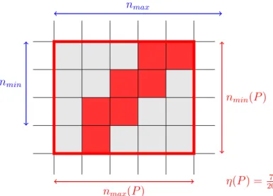
3.10 Some input parameters for patch creation algorithms . . . 68
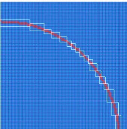
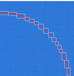
3.11 Bubble-liquid interface covered by patches with the Berger-Rigoutsos method . . . 71
3.12 Bubble-liquid interface covered by patches with the Livne method . . . 72
3.13 Bubble-liquid interface covered by patches with the nmin – nmax method . . . 73
3.14 Exchange pattern for just two levels . . . 75
3.15 Exchange pattern for more than two levels: “two times V” strategy . . . 75
3.16 Exchange pattern for more than two levels: “W” strategy . . . 75
3.17 Ellipsoidal bubbles covering test cases . . . 81
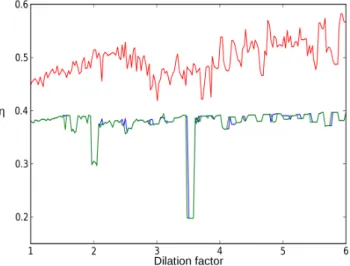
3.18 Resulting efficiency η, as a function of the dilation factor and of the patch creation algorithm (higher is better) . . . 82
3.19 Normalised standard deviation σ, as a function of the dilation factor and of the patch creation algorithm (lower is better) . . 83
3.20 Average squareness γ, as a function of the dilation factor and of the patch creation algorithm (higher is better) . . . 83
3.21 Intersection of Ω□(itert = 0) and Ω□(itert= 1) . . . 93
3.22 Flowchart for AMR on two levels . . . 95
3.23 Advected bubble visualised with its 3D patches . . . 97
3.24 Speedup for the 1.7 billion cells test, for all algorithms . . . . 98
3.25 Speed-up for the 1.7 billion cells test . . . 99
3.26 Speedup for the 4 billion cells test . . . 100
4.1 Nomenclature for areas in Ω = Ω□∪ Ω⃝ . . . 103
4.2 Nomenclature for grids in Ω = Ω□∪ Ω⃝ . . . 103
4.3 Nodes of Ωc . . . 104
4.4 Localisation of grid nodes, r = 4 and ϑ = 1 4 . . . 105
4.5 LDC algorithm on nodes, with one patch . . . 107
4.6 Nodes of ΩH def . . . 109
4.7 Location of the centre of the cells of the coarse grid ΩH . . . . 116
4.8 Location of the centre of the cells of the fine grid Ωh □ . . . 117
4.9 Location of ghost cells, for nGC = 1 and r = 2 . . . 117
4.10 LDC algorithm on cells, with one patch . . . 119
4.11 Two patches touching each other . . . 121
4.12 LDC algorithm on cells, with Schwarz domain decomposition . 122 4.13 2D Zalesak disk . . . 124
4.14 Y field at t = 0, 2D case . . . 125
4.15 Y field at t = 0, 3D case: zoom on a corner of Ω . . . 125
4.16 Y field at t = 3.12, 2D case . . . 126
4.17 Y field at t = 3.046, 3D case: zoom on a corner of Ω . . . 127
4.18 Volume of the bubble as a function of time, for a 30× 30 grid, without AMR . . . 128
4.19 Volume of the bubble as a function of time, for a 60× 60 grid, without AMR . . . 128
4.20 Volume of the bubble as a function of time, for a 30× 30 grid, with AMR refinement of 2 . . . 129
4.21 CDMATH architecture . . . 131
4.22 Logo of the CDMATH workgroup . . . 132
5.1 Location of coordinates . . . 134
5.2 Final state of lid-driven cavity simulation (streamlines of u) . 152 5.3 Final state of lid-driven cavity simulation (isocontours of ||u||) 153 5.4 Intermediary state of lid-driven cavity simulation (with white AMR patch, streamlines of u and isocontours of ||u||) . . . 154
5.5 ux along vertical axis, as a function of y . . . 155
5.6 uy along horizontal axis, as a function of x . . . 156
5.7 Initial state for two-fluid incompressible Navier-Stokes simu-lation, with AMR patches shown as white rectangles . . . 164
5.8 Intermediary state for two-fluid incompressible Navier-Stokes simulation, with AMR patches shown as white rectangles . . . 165
6.1 Mushroom-shaped Rayleigh-Taylor instability . . . 168
B.1 log(L2error) as a function of log(∆x∆y) . . . 179
C.1 Test 2D de Kothe-Rider, avec patchs AMR visibles . . . 184
C.2 Schéma simplifié de l’algorithme LDC . . . 186
C.3 Simulation de la cavité entraînée (isocontours de ||u||) . . . . 188
C.4 Simulation de deux bulles, avec les patchs AMR affichés en rectangles blancs . . . 190
List of Tables
2.1 Kinematic viscosity of liquid water for different temperatures . 41 2.2 Classification of approximations . . . 48 3.1 Input parameters for our ellipsoidal bubble test cases . . . 82 3.2 Comparison of the average of quality functions of each
al-gorithm on a series of tests (+ standard deviation of quality function) . . . 84 3.3 Input parameters for our 1.7 billion cells Kothe-Rider test . . 97
Nomenclature
⋆0 As a subscript: relative to the initial conditions
1 Indicator function
A Matrix for predicted velocity
α Void fraction
A Operator for the computation of the AMR patch covering
b Right hand side for predicted velocity
⋆BC As a subscript: relative to boundary conditions
⋆c As a superscript: relative to the composite grid
C Matrix for potential
c Speed of sound
d Right hand side for potential
∆t Time step
∆x Elementary grid space
𝟋 Dilation factor
E Specific energy
e Internal energy
η Patch efficiency
^ex Elementary unit vector along direction x
^ey Elementary unit vector along direction y
^ez Result of the cross-product ^ex× ^ey
F Volumetric force
f Force acceleration
F Operator for initial conditions from an analytic formula
g Gravitational acceleration
⋆g As a subscript: relative to the gas phase
γ Average squareness
γ Ideal gas factor
GC Set of ghost cells
⋆H As a superscript: relative to the coarse grid
⋆h As a superscript: relative to the fine grid
i Space index along x
I Space index along x, specifically for the coarse grid Ih Interpolation from coarse to fine
ij Matrix index
iter Iteration
iterLDC Iteration of LDC algorithm
iterSch Iteration of Schwarz algorithm
j Space index along y
k CFL stability coefficient
κ Curvature
L Linear elliptic second-order differential operator
⋆l As a subscript: relative to the liquid phase
L Length
λ Thermal transfer coefficient
M Mach number
M Set of matrices
M Averaging operator
µ Volumetric viscosity
n Time index
nmax Maximum number of cells in any direction of a patch
nmin Minimum number of cells in any direction of a patch
N Total number of cells of a patch
n Normal vector
ν Kinematic viscosity
Ω Computational domain
∂Ω Border of the computational domain
O Time resolution to get the state itert+ 1 from the state itert
Or The O operator composed r times with a time step ∆t
r
P Thermodynamic pressure Π Dynamic pressure φ Level-set function ϕ Potential ψ Pulsation r Refinement coefficient R Radius R Reynolds number
RH Restriction from fine to coarse
ρ Volumetric mass
ϱ Distance to the origin
s Source
S Surface
S Smoothing operator
Σ Interface
σ Normalised standard deviation
ς Signature in a patch su Computation speed-up t Time T Temperature T Duration t Tangential vector
τ Stress tensor
τsurf Surface tension coefficient
θ Coefficient of thermal dilation
Tsurf Surface tension
u Velocity
U Velocity parallel to faces
ũ Predicted velocity
V Volume
x Spatial position
ξ Spatial position in another referential
Y Colour function
⋆□ As a subscript: relative to the local refined area
Chapter 1
Introduction
1.1 Purpose of this research: two-phase flows
in nuclear reactors
To a large extent, producing electricity with a nuclear power plant resembles a lot how one produces energy with other types of power plants, in particular fossil fuel plants like the ones using coal or gas. The base principle could be summarised as follows: using a thermal source, water is heated up, circulates and transmits its heat to a vapour phase, which then makes a turbine turn. This is a transmission of thermal energy into kinetic energy; the turbine creates electricity with a dynamo-effect and the electricity is transported to the customers. In the case of nuclear power plants, the thermal source takes its origin in the core of the power plant where the nuclear chain reaction takes place. In the end, what makes the Nuclear Engineering field a complex one is the combination of multiple physics fields: nuclear physics, thermal-dynamics, hydrothermal-dynamics, material science, solid mechanics, chemistry (e.g. for the fission products), electrical engineering and so forth. The engineering challenge of the scale of the phenomenons comes on top of that: extreme heat, flow rates and turbine rotation speeds for instance.
The Thermal-Hydraulics study of two-phase flows is a major topic for Nuclear Engineering because it contributes to improving the safety and the efficiency of reactors. It is the study of mixtures of liquid water and steam in nominal regime as well as in accidental regime. The first most common nuclear power plant design is the Pressurised Water Reactor (PWR). Figure 1.1 represents a commercial PWR nuclear power plant and Figure 1.2 shows
Figure 1.1 – Representation of a commercial nuclear plant [62]
the components for a second-generation submarine nuclear propulsion sys-tem. In red, we have the primary loop; the nuclear reaction takes place in the core and transmits the generated heat to the water. In blue, we have the secondary loop; including the steam generators where most if not all the boiling takes place. The two loops are separated with a physical barrier to avoid any eventual contamination by radioactive material detaching from the core. In a normal regime, the water flow inside the primary flow of a PWR is kept liquid thanks to the immense pressure. An eventual vapour phase may nonetheless appear in some conditions, like accidental ones or in the case of meta-stable bubbles from a thermal-dynamics point of view. On the opposite, steam is supposed to appear in the secondary loop, by design. So for safety reasons, it is important to study when and where the steam may appear and to analyse its behaviour.
The other most common nuclear power plant design is the Boiling Water Reactor (BWR). As its name indicates, the flow inside the core of a BWR is by design made of a mixture of liquid water together with steam. This is why it is essential to study two-phase flows in the core of PWRs and BWRs. Similarly, one of the components of PWRs in addition to the nuclear core is the steam generator. This is the location of the boiling, producing the steam which will make the turbines turn and hence produce electricity. For this component the purpose is to understand and predict precisely where the
Figure 1.2 – Representation of a submarine propulsion system [68]
boiling takes place. In particular, the area called the Departure of Nucleate Boiling (DNB), where the first bubbles are born, is of foremost importance [27]. An accurate knowledge of its location would permit to increase effi-ciency. A finer comprehension of the mechanisms of a production unit and a better efficiency will lead to an optimisation of the output and thus a more consequent turnover and profitability, in addition to safety.
Because of the aforementioned stakes, many efforts have been put on the physical aspect of two-phase flows. This means that research laboratories and companies lead many physical experiments to gather knowledge. Examples of those are MISTRA at CEA in Saclay, France [43, 134], and PKL at AREVA in Erlangen, Germany [11]. The experiments permit to get invaluable data and know-how for the dimensioning work for future designs. In addition to experiments, numerical modelling also helps for knowing precisely when and where phenomenons appear in the different parts of a power generation unit. It is crucial for the design of new components [144], for the day-to-day opera-tion of reactors, as well as for the comprehension of past operaopera-tional regimes, incidents and accidents [92]. For instance, instead of some ten physical very expensive and difficult to manufacture physical experiments, we can try to replace them with hundreds of numerical experiments and just a few physical ones for calibration and validation.
System Component Local 3D Local instantaneous (DNS) Need more effort in physical modeling
Need more power for computation
Figure 1.3 – Successive scales for modelling [83], [62], [30]
1.2 Different numerical simulation scales to
model nuclear Thermal-Hydraulics
The numerical simulation of Thermal-Hydraulics is of primary importance for Nuclear Engineering for both security and efficiency of nuclear facilities at all scales [135]. The thermal-hydraulicists who try to represent flows in a nuclear context work on different modelling scales, represented on Figure 1.3. We can order them from largest to finest [83]:
1. system scale 2. component scale 3. local 3D scale
4. local instantaneous scale (DNS)
The system scale aims at representing the whole energy production unit, including in particular the reactor, the steam generators and all other pipes. It is the macro-scale used in well-known nuclear codes, like CATHARE [28], RELAP [25] or ATHLET [34]. This scale requires a large effort in physical modelling and that is why Thermal-Hydraulics equations are often used in their 0D expression.
The component scale aims at representing only a part of the plant: ex-amples of codes for this scale include GENEPI [109], FLICA [137].
The local 3D scale is much finer and is related to Computational Fluid Dynamics. It is appropriate for the representation of problems with a size ranging from a few meters to a few tens of centimetres. For instance, Bieder et al. used Trio U for the simulation of flows around nuclear fuel bundles [29]. The final scale is Direct Numerical Simulation. It is appropriate for the representation of problems with a size ranging from a few tens of centimetres
to a few millimetres. At this scale, we can represent the interface between liquid and vapour; it is very applicable to bubble problems [40].
Given the sizes of a nuclear core, most if not all nuclear codes represent two-phase flows in an averaged manner. This means that the liquid-vapour interface is not explicitly represented in the models and the codes. Such averaged models thus require closure laws modelling mass, momentum and heat transfer between phases. In order to get such laws, physical experi-ments are of course necessary. Nonetheless, thanks to the improvement of computation capabilities, we can now hope to take advantage of fine numer-ical simulation like DNS because they explicitly represent the deformations of the liquid-vapour interfaces.
1.3 Outline and summary of the thesis
Note: Appendix C contains the translation into French of this section about the outline and the summary of the thesis.
1.3.1 Models of flows with two separated phases
In this thesis we start in Chapter 2 with explaining a series of existing thermal-hydraulics models, with a focus on two separated phases. We start with the common compressible models: Euler and Navier-Stokes systems. We explain the first one with only one phase in Section 2.1.1, the second one with two phases in Section 2.1.2. In Section 2.1.3, we then make the hypo-thesis of incompressibility, to get the incompressible Navier-Stokes model:
∂tu + u· ∇u − ν∇2u = f =− 1 ρ∇p + g + fothers, ∇ · u = 0, u = uBC on ∂Ω (boundary conditions),
u(t = 0) = u0 on Ω (initial conditions).
(1.1)
Equation (1.1) gives the expression for one phase, with notations thoroughly defined further in the thesis. The expression for two phases is given by
Equation (1.2): ∂tu + u· ∇u − ν∇2u = f =− 1 ρ∇p + g + fothers, ∇ · u = 0, ∂tY + u· ∇Y = 0, ρ = ρgY + ρl(1− Y ), u = uBC on ∂Ω (boundary conditions),
u(t = 0) = u0 on Ω (initial conditions),
Y (t = 0) = Y0 on Ω (initial conditions).
(1.2)
We go on in Section 2.1.4 with the models used in nuclear codes, the 6-and 7-equation models, also referred to as mixture models. In Section 2.1.5, we focus on low-Mach number conditions; when the flows go at low speed compared to the speed of sound. We review the Diphasic Low Mach Number model, proposed for nuclear conditions too. Finally we present in Section 2.1.6 the Abstract Bubble Vibration model, a coupling between an hyperbolic equation and an elliptic equation.
When interested in the DNS of bubbles, we have to get the right tools to numerically model the interface. We present in Section 2.2 two important techniques. Front tracking, as explained in Section 2.2.1, is modelling the flow with a convective (or “Lagrangian”) perspective. On the opposite, as explained in Section 2.2.2, we relate front capturing to a Eulerian perspective. We explain why we choose the latter. Our implementation is the transport of a colour function Y which equals either 1 in the gas phase, or 0 in the liquid phase. We will have to find the right discretisation scheme to keep the jump from 1 to 0 as sharp as possible.
1.3.2 Front capturing with AMR: finite differences schemes
and parallelisation
We show in Chapter 3 that Direct Numerical Simulation is the most precise scale of computation and therefore also the most expensive one. Adaptive Mesh Refinement is the enrichment of a subset of the computational domain
Figure 1.4 – 2D Kothe-Rider test, with AMR patches visible
– the area of interest – with more detail. We explain how AMR is beneficial to DNS by reviewing a part of the mesh refinement literature. In Section 3.1, we differentiate the following techniques: anisotropic meshing, r-adaptation, p-adaptation, h-p-adaptation, s-adaptation. We decide to focus on patch-based mesh adaptation on Cartesian grids in Section 3.2. This means that we cover the said area of interest with one or several levels of patches, which have a finer space discretisation. Figure 1.4 shows a standard test case for advection equations, the 2D Kothe-Rider test [119]. We used patch-based AMR with one level of refinement. We show the coarse level (in fact, the entire computational domain) inside a green square, it is discretised with a 100 × 100 grid. We show the fine level inside the many white rectangles, which are patches with a refinement coefficient r = 4. They cover the area we determined of interest: the interface between liquid and gas. We can say that the simulation has an equivalent discretisation of 400 × 400.
We present multiple ways to define the patches; the Berger-Rigoutsos algorithm [22], the Livne algorithm [99]. We also propose our own improve-ment, the nmin – nmax algorithm. It constrains the size of the patches with
be-ing the minimum efficiency ηmin of the covering. We introduce three quality
functions to compare patch coverings: the average efficiency η, the normal-ised standard deviation of sizes σ and the average squareness γ. We compare the three algorithms in a multiprocessing perspective in Section 3.3. For this we determine the value of the quality functions on a few hundreds of test coverings using the three algorithms. We settle for nmin – nmax. We
decide to test out our choice in Section 3.4 with a 3D Kothe-Rider advection simulation. We present different advection schemes, including the upwind scheme and WENO. We choose the limited downwind scheme introduced by Després and Lagoutière [51], because it captures and transports the colour function Y in a very sharp manner. By locating the refinement patches on the interface between liquid and gas, we get encouraging results as far as computational speed-up is concerned when we use parallel computing.
1.3.3 Elliptic equations and Abstract Bubble
Vibra-tion model
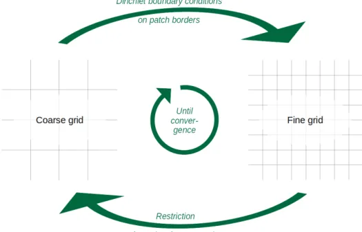
As we explain in Chapter 4, elliptic equations are more challenging to repres-ent with patch-based AMR, since they require information from the whole computational domain. This is why, in Section 4.1, we choose to use the Local Defect Correction algorithm [74]. As schematically presented on Fig-ure 1.5, LDC is an iterative process done until we determine that we reached convergence. At each iteration, the computed solutions of the coarse and the fine (patch) grids enrich one another. The computed solution on the coarse grid defines Dirichlet boundary conditions on the borders of the patches. We then solve the elliptic equation with the said boundary conditions on the fine grid. The computed solution of the fine grid permits to calculate the eponymous Local Defect Correction on the refined area: it will replace the source term of the coarse level, eventually leading to a new coarse resolution and a new LDC iteration.
In the following section, we recall the proof of its convergence laid out by Ferket et al. [63] and Anthonissen et al. [10]. We then propose our variant of LDC, differing from the literature in two ways. First, we use cell-centred values and not values on nodes of the meshes. Therefore, for the Dirichlet boundary conditions interpolation step from coarse to fine, we provide the patches with ghost cells around their border. Second, most of the time, we deal with multiple patches, often touching each other. So we decide to consider them as a partition of the fine level: we use the Schwarz iterative algorithm of domain decomposition to determine an acceptable solution of
Figure 1.5 – Schematic representation of the LDC algorithm
the fine level, with no discontinuity at the interface between patches. We test our implementation out with the ABV model in Section 4.2, in 2D as well as in 3D. We locate the patches on the interface of the bubble. We use a formula giving the volume of the bubble as a function of time to verify that we get convincing results. We implemented the AMR tools we used in an open-source library named CDMATH and conceived to help other computational scientists and engineers [44, 145]. We present how CDMATH was designed and how AMR is an extension in Section 4.3. With this toolbox, one can implement AMR as easily in 2D as in 3D.
1.3.4 Application to incompressible Navier-Stokes
Finally, we apply in Chapter 5 the result of our work on Adaptive Mesh Re-finement to more realistic simulations. We represent incompressible Navier-Stokes systems on staggered grids (scalar variables located at the centre of cells, vectors located at the faces). We use one level of AMR. In Section 5.1, we fully detail the numerical schemes for a one-phase simulation of Equation (1.1). In the thesis, we detail the following prediction-correction scheme, in
the spirit of the work of Chorin [38, 39] and Temam [131, 132]: ũ− un ∆t + u n· ∇ũ − ν∇2ũ = fn= g− 1 ρ∇p n, ũ = ũBC on ∂Ω, ũBC · n = uBC · n, ũBC · t = uBC· t + ∆t ρ ∇ϕ n· t. (1.3) −1 ρ∆ϕ n+1 =− 1 ∆t∇ · ũ, ∇ϕn+1· n = 0 on ∂Ω. (1.4) pn+1 = pn+ ϕn+1. (1.5) un+1− ũ ∆t =− 1 ρ∇ϕ n+1, un+1 = u BC on ∂Ω. (1.6)
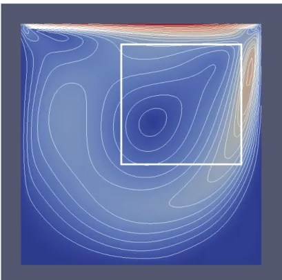
As explained later, we use the LDC algorithm to finely compute the incre-ment of pressure ϕ. We see that it is essential the source term of Equation (1.4) – namely the divergence of the predicted velocity ∇ · ũ – be linearly interpolated from the coarse level onto the fine level. We verify our imple-mentation using the classic literature test case of the lid-driven cavity. A permanent regime exists and is well known beforehand: depending on the Reynolds number, several whirlpools are created in the computational do-main, so we placed one refinement patch on the main whirlpool. Figure 1.6 represents the permanent regime, with the colouring as a function of the ve-locity||u|| and the isocontours of ||u|| given as white lines. We represent the location of the fine level patch by a white square. A video of the transitional regime can be seen online at https://youtu.be/esOHN--iW4Y.
In Section 5.2, we switch to two-phase situations, represented by Equation (1.2). We also use staggered grids, with one exception though: we locate the inverse(1
ρ
)
of the volumetric mass at the faces and not at the centre of cells, although it is a scalar. Here too we use a prediction-correction scheme which
equations are fully explained in the thesis: ũ− un ∆t + u n· ∇ũ − ν∇2ũ = gn+1− 1 ρn∇p, ũ = uBC on ∂Ω. (1.7) −∇ · ( 1 ρn∇ϕ n+1 ) =− 1 ∆t∇ · ũ, ∇ϕn+1· n = 0 on ∂Ω. (1.8) pn+1 = pn+ ϕn+1. (1.9) un+1− ũ ∆t =− 1 ρn∇ϕ n+1 , un+1= u BC on ∂Ω. (1.10) Yn+1− Yn ∆t + u n+1· ∇Yn = 0. (1.11) ρn+1 = ρgYn+1+ ρl(1− Yn+1). (1.12)
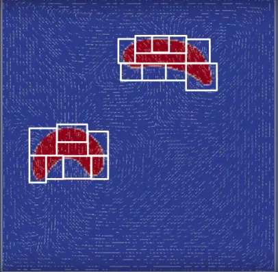
As for the one-phase simulation, we use one level of Adaptive Mesh Refine-ment. We create the patches dynamically at every time step and locate them such that they follow the interface between gas and liquid, as in Chapters 3 and 4. We propose an original AMR approach that benefits from the work done earlier. We first decide to compute the increment of pressure ϕ with the LDC algorithm applied on Equation (1.8), which is elliptic. Then we decide to compute the hyperbolic advection of Equation (1.11) with AMR precision too. We explain why it is essential that we interpolate the source term∇ · ũ of Equation (1.8) from the coarse level to the fine level. As a consequence, we have a precise computation of the variables ϕ, p, Y and ρ at the location of their discontinuities or jumps of derivative. In addition, in spite of the sharp jump of the presence Y , we are able to give a satisfying model for surface tension of bubbles. This lets us obtain realistic evolutions of non-stationary bubbles due to gravity, viscosity, inertia, surface tension, pressure forces. Figure 1.7 is a shot of such a simulation, which video can be seen online at https://youtu.be/zJEjP6JYEYQ. We can see the AMR patches as white rectangles on the interfaces and the streamlines of the velocity as white little arrows.
Figure 1.7 – Simulation of two bubbles, with AMR patches visible as white rectangles
1.3.5 Outreach
The last chapter, Chapter 6 is just the listing of our communications realised during the PhD, as well as of supervising and funding institutions.
Chapter 2
Models of flows with two
separated phases
2.1 Thermal-Hydraulics models adapted for
each scale
In this section we present a few physics models used to represent one-phase and two-phase flows.
For all models, we will use the same denomination of spatial areas of the problem, represented on Figure 2.1. We will also use the same initial conditions.
We name the computational domain Ω and we name its border ∂Ω. The volume of Ω is written |Ω|. We partition the space into two: Ω = Ωl ∪ Ωg.
The space Ωl represents the domain of Fluid l, typically a liquid. The space
Ωg represents the domain of Fluid g, typically a gas.
Let x be the vector positioning in space and let t be the time. We define the colour function Y (x, t) as an indicator for the gas phase:
∀(x, t) ∈ Ω × R+, Y (x, t) =
{
1 if x∈ Ωg (i.e. gas/vapor),
0 if x∈ Ωl (i.e. liquid).
(2.1)
So we can express the initial conditions for Y as follows:
∀x ∈ Ω, Y (x, t = 0) =
{
1 if x∈ Ωg(t = 0),
0 if x∈ Ωl(t = 0).
Ω
l(t)
Ω
g(t)
Σ(t)
u
W .w al lu
E .w al lu
N.wallu
S.wall Figure 2.1 – Ω(t) = Ωl(t)∪ Ωg(t)We also define Σ(t) the interface separating liquid and gas. It may evolve with time, appear in some places or disappear in others.
Let the scalar T (x, t) be the temperature and p(x, t) the local pressure of the fluid. We call “normal temperature and pressure conditions” the couple (T, p) where T = 25◦C and p = 1.024 bar. Let the scalar ρ(x, t) be the volumetric mass. For liquid water at normal temperature and pressure con-ditions, ρwater = 1000 kg m−3. Let the vector u(x, t) be the local velocity of
the fluid. Then ρu represents the local volumetric momentum.
The vector F represents physical volumetric forces. In our case, the forces include at least pressure forces, gravity and eventually other sources Fothers.
Let f be the expression of these forces divided by the volumetric mass ρ:
f is homogeneous to an acceleration. As an example, the vector g is the
gravitational acceleration, with a norm||g|| = 9.8 m s−2. Let τ be the stress tensor, with Stokes’ hypothesis. The scalar µ is the volumetric viscosity and the scalar ν is the kinematic (i.e. specific or massic) viscosity coefficient;
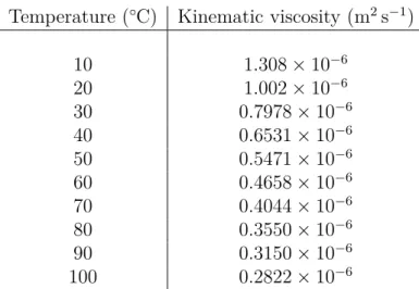
ν = µρ. For instance, for liquid water at 25◦C, νwater = 10−6m2s−1. Table
Temperature (◦C) Kinematic viscosity (m2s−1) 10 1.308× 10⁻⁶ 20 1.002× 10⁻⁶ 30 0.7978× 10⁻⁶ 40 0.6531× 10⁻⁶ 50 0.5471× 10⁻⁶ 60 0.4658× 10⁻⁶ 70 0.4044× 10⁻⁶ 80 0.3550× 10⁻⁶ 90 0.3150× 10⁻⁶ 100 0.2822× 10⁻⁶
Table 2.1 – Kinematic viscosity of liquid water for different temperatures Let E be the specific energy, ρE the volumetric energy and e be the specific internal energy. Let λ be the thermal transfer coefficient.
2.1.1 One-phase compressible Euler system
For two given vectors u and v, let us define u· ∇v as follows:
u· ∇v = (u · ∇) (v) ,
= (ux∂x+ uy∂y+ uz∂z) (v) .
(2.3) The one-phase compressible Euler system is given by the following set of equations (written using a non-conservative formulation):
∂tρ +∇ · (ρu) = 0, ∂tu + u· ∇u = − 1 ρ∇p + g, ∂te + u· ∇e + p ρ∇ · u = 0. (2.4)
The first equation is the conservation of mass, the second one is the transport of momentum, and the last one is the transport of internal energy. To close the system of Equations (2.4), we add the equation of state as well: this is an algebraic equation that establishes the relationship between the pressure
functionEOS, the equation of state can take the general formulation:
EOS(p, e, ρ) = 0. (2.5)
For instance, let us consider that the fluid is a Laplace ideal gas. Let us call
γ the ideal gas factor, equal to the heat capacity at constant volume divided
by the heat capacity at constant pressure. The quantity γ is equal to 5 3 if
the Laplace ideal gas is a monoatomic gas (like helium He) and γ = 7 5 if the
gas is diatomic (like nitrogen N2). In this case we can use the ideal gas law
as the equation of state:
EOS(p, e, ρ) = p − ρe(γ − 1) = 0. (2.6) As far as the boundary conditions are concerned, let Ω be bounded by immobile walls. The boundary conditions for the Euler system are a little complicated to write down. In particular, they depend on where and when the velocity is directed into the domain.
2.1.2 Two-phase compressible Navier-Stokes model
We can represent the two-phase compressible Navier-Stokes equations with the following set of four equations:
∂tY + u· ∇Y = 0, ρ = ρgY + ρl(1− Y ), ∂tρ +∇ · (ρu) = 0,
∂t(ρu) +∇ · (ρu) = −∇p + ∇ · τ(u) + ρg,
∂t(ρE) +∇ · [(ρE + p)u]
=∇ · (λ∇T ) + ∇ · [τ(u)u] + ρg · u.
(2.7)
The first equation is the transport of the colour function Y . It is expressed in a non-conservative way which satisfies a maximum principle for Y . The second equation gives the volumetric mass ρ as a function of the presence of the two phases. The third equation is the conservation of said ρ. The fourth equation is the conservation of the volumetric momentum ρu. The fifth and last equation is the conservation of volumetric energy ρE. In addition, we also have the equation of state for the relationship between Y , p, e given by
e = E− 12u2 and ρ. Let EOSk(p, e, ρk) = 0 be the equation of state of each
phase k = l and k = g. Multiple choices are possible for the equation of state of the mixture [46, 62]. We may for instance choose the following equation defining EOS(Y, p, e, ρ):
EOS(Y, p, e, ρ) = (1 − Y )EOSl(p, e, ρl) + YEOSg(p, e, ρg) = 0. (2.8)
We choose the value of all the coefficients depending on the phase, such as transport and thermodynamic coefficients, as a function of Y . Let ξ be a coefficient as for instance λ, α, Cp and others:
ξ(Y, T, p) = (1− Y )ξl(T, p) + Y ξg(T, p). (2.9)
For instance, we have the following equality for λ:
λ(Y, T, p) =
{
λl(T, p) if x∈ Ωl(t) (i.e. Y = 0),
λg(T, p) if x∈ Ωg(t) (i.e. Y = 1).
(2.10)
As far as the boundary conditions are concerned, Ω is bounded by im-mobile walls. There are many types of possible boundary conditions, as for instance Neumann or Robin ones. We decide to focus on Dirichlet boundary conditions. Let uBC be a boundary conditions given for the velocity u:
∀x ∈ ∂Ω, u(x, t) = uBC. (2.11)
We choose to have walls that can only move in the direction they occupy, as shown on Figure 2.1. In other words, a wall along the x axis can only move in the x direction. Furthermore, we impose no-slip conditions, so uBC = uwall.
However, if the speed on the walls is not zero, then we have to choose entry conditions on the boundaries for the advection contributions.
We also choose to have adiabatic conditions:
∀x ∈ ∂Ω, ∇T (x, t) · n(x) = 0 (2.12) where n is the vector normal to the wall ∂Ω.
The compressible Navier-Stokes system is adapted for problems where acoustic shock waves appear and should be represented correctly. Kokh presents this particular two-phase compressible Navier-Stokes system – but also other ways to model the interface – in his PhD thesis [89]. As a final note, the Euler system (2.4) can be seen as a Navier-Stokes system where we make the viscosity ν equal to zero.
2.1.3 Incompressible Navier-Stokes model
The incompressible Navier-Stokes model accounts for the conservation of (volumetric) momentum ρu in fluids which density (or volumetric mass) ρ is constant in time and uniform by pieces in space. In particular, ρ only depends on the species of the fluid. Thus it cannot model large thermal dilation nor pressure shock waves.
The one-phase incompressible Navier-Stokes model is hence given by the following set of equations:
∂tu + u· ∇u − ν∇2u = f =− 1 ρ∇p + g + fothers, ∇ · u = 0, u = uBC on ∂Ω (boundary conditions),
u(t = 0) = u0 on Ω (initial conditions).
(2.13)
The vector u0 is an initial condition given for the velocity u and verifying
∇ · u0 = 0.
We numerically solve an example of this one-phase model in Section 5.1.
For the two-fluid incompressible Navier-Stokes model, we consider two fluids: Fluid l and Fluid g. As a consequence, ρ is constant in time and uniform by pieces in space. The density is attached to the colour function
Y . The scalar ρ equals ρl in areas where Y = 0 and equals ρg in the other
areas, where Y = 1. The colour function Y thus indicates the presence of Fluid g. The scalar Y is transported by the velocity u (defined on all the
computational domain), which brings us to the following set of equations: ∂tu + u· ∇u − ν∇2u = f =− 1 ρ∇p + g + fothers, ∇ · u = 0, ∂tY + u· ∇Y = 0, ρ = ρgY + ρl(1− Y ), u = uBC on ∂Ω (boundary conditions),
u(t = 0) = u0 on Ω (initial conditions),
Y (t = 0) = Y0 on Ω (initial conditions).
(2.14)
We numerically solve an example of this two-fluid model in Section 5.2.
2.1.4 Mixture models: the 6- and the 7-equation
mod-els
An abundant category of two-phase flow models is mixture models. Those consider that for every point in space (and every discretisation volume sur-rounding it), one can define a void fraction α. For an elementary space of a volume V and containing a volume Vg of gas, the following formula gives the
void fraction:
α = Vg
V . (2.15)
Mixture models are thus “homogenised” or “averaged” models where for each point x in space, both phases coexist. We understand that mixture models are adapted to larger scale problems.
The 6-equation model, also sometimes named the two-fluid model, is used for instance in the nuclear code CATHARE. It is based on a set of 6 equations of conservation [28].
The conservation of mass of each phase reads as follows:
∂
∂t(αgρg) +∇ · (αgρgug) = 0, ∂
∂t(αlρl) +∇ · (αlρlul) = 0.
The conservation of momentum of each phase reads as follows: ∂ ∂t(αgρgug) +∇ · (αgρgug⊗ ug) + αg∇p = Fg, ∂ ∂t(αlρlul) +∇ · (αlρlul⊗ ul) + αl∇p = Fl. (2.17)
Finally, the conservation of momentum of each phase reads as follows:
∂
∂t(αgEg) +∇ · (αgEgug) + αg∇ · (pug)
={Net energy exchange with the environment}g
+{Net energy generation}g, ∂
∂t(αlEl) +∇ · (αlElul) + αl∇ · (pul)
={Net energy exchange with the environment}l
+{Net energy generation}l.
(2.18) The system is completed with closure laws. One of the drawbacks of this model is that it may show non-hyperbolicity problems (see [128] for instance). Without going into too many details, let us consider the 7-equation model which unconditionally solves the non-hyperbolicity problems. This model is called Baer-Nunziato, introduced in [14]. The model is further studied in [67, 45] and schemes specific to the model are presented in [6, 41]. It introduces an interface pressure pΣ and an interface velocity uΣ. Let k refer to the fluid
g or l. Then the conservation laws rewrite as follows: ∂αk ∂t + uΣ· ∇αk= µ(pk− pΣ), (2.19) ∂ (αkρk) ∂t +∇ · (αkρkuk) = 0, (2.20) ∂ (αkρkuk) ∂t +∇ · (αkρkuk⊗ uk) +∇(αkpk) = pΣ∇αk+ λ(uk− uΣ), (2.21) ∂ (αkρkEk) ∂t +∇ · ( (αkρkEk+ αkpk)uk ) = pΣuk· ∇αk+ λuΣ(uk− uΣ) + µpΣ(pk− pΣ). (2.22) We can notice that Equation (2.19) is a transport of the void fraction plus a relaxation term.
In practical simulations, the relaxation parameters λ and µ are very small (10−8), the interface pressure pΣ is taken as the largest pressure of the fluids
and the interface velocity uΣ is taken equal to the velocity of the other fluid
Tmatter
Tacoustic
· · ·
Figure 2.2 – Characteristic durations
2.1.5 The Diphasic Low-Mach Number model
Low-Mach flow conditions
In most situations, there are two very distinct time scales in thermal-hydrau-lic flows. The first one is the time scale of pressure shocks and other acoustic phenomenons. Typically, the order of magnitude of the phenomenons nears
Tacoustic ≃ 10−3s. The second time scale is related to how fast the matter
– the fluid in itself – flows along pipes etc. It is typically of the order of magnitude of Tmatter≃ 1 s in nuclear cores.
These two time scales are very different one from another, as represented on Figure 2.2. This brings specific difficulties:
1. the precision in schemes (e.g. the Godunov scheme has a poor precision in low-Mach number conditions on Cartesian grids),
2. the robustness of solvers (for instance, inverting matrices with very different eigenvalues is hard with usual iterative methods, because of the bad conditioning; this is indeed the case at low Mach number). We define the Mach number as follows:
M = ||u||
c . (2.23)
The module||u|| is the velocity of the fluid matter (or a magnitude thereof). The quantity c is the speed of sound. In a nuclear reactor in particular, we are in low-Mach number conditions in the vast majority of cases, be it in nominal regime or in many accidental regimes like Loss Of Flow Accidents for example: M = ||u||c ≃ 10−3.
As a consequence, we can say we can neglect shock waves and other acous-tic phenomenons.
However thermal phenomenons do remain important: due to thermal dila-tion, ∇ · u ̸= 0 although M ≪ 1.
M ≪ 1 M ≪ 1 M = O(1) ||∇ · λ∇T || ≪ 1 ||∇ · λ∇T || = O(1)
Incomp. Navier-Stokes ≤ Low-Mach asymptotic model < Comp. Navier-Stokes
×acoustic ×acoustic ✓acoustic
×thermal ✓thermal ✓thermal
Table 2.2 – Classification of approximations
Table 2.2 summarizes a classification of models. On the far right, we have the compressible Navier-Stokes model, which takes into account all phe-nomenons (acoustic and thermal). The Mach number M may be large. See Section 2.1.2. On the far left, we have the incompressible Navier-Stokes model, which neglects acoustic as well as thermal phenomenons. See Section 2.1.3. In between, we are searching for a model which neglects acoustic phe-nomenons but still represents thermal dilation. This would be the low-Mach asymptotic model presented hereafter.
Low-Mach number approximation: DLMN model
The Diphasic Low-Mach Number (DLMN) model [47, 46] takes its inspir-ation from previous work about combustion, dating back at least since the seventies; see for instance [100]. Low-Mach number models have also been used in many other fields, as for instance in Cosmology [5] or Microfluidics for electronic systems [118]. It was then proposed for Nuclear Reactors Thermal-Hydraulics [48, 76]. Penel studied the model from a theoretical and analytic point of view [113, 114].
We can show that, when the Mach number M is small, we can approxim-ate the two-phase compressible Navier-Stokes model (as presented in Section 2.1.2) with the DLMN model. Let θ be the coefficient of thermal expansion:
θ(Y, T, p) =−1 ρ
∂ρ
∂T(Y, T, p). (2.24)
In this model, we keep the transport equation for Y . We replace the energy equation with the transport equation for internal enthalpy. We have a con-servation equation for momentum. At last, we have a coupling equation of constraints with all other equations. This leads us to the following system of
equations: ∂tY + u· ∇Y = 0, ρCp(∂tT + u· ∇T ) = θT P′(t) +∇ · (λ∇T ), ρ(∂tu + u· ∇u) = −∇Π + ∇ · τ(u) + ρg, ∇ · u = G(x, t), G(x, t) =−P ′(t) ΓP (t)+ β P (t)∇ · (λ∇T ), β = θP ρCp , Γ = ρc 2 P , P′(t) = ∫ Ω β(Y, T, P )∇ · λ∇T dx ∫ Ω dx Γ(Y, T, P ) . (2.25)
The quantity P is a pressure depending only on time and equations of state. In this model, P is the “thermodynamic pressure” and does not depend on the spatial coordinate x. The coefficient of thermal dilation now depends on P : θ = θ(Y, T, P ). The quantity Π is a perturbation of the pressure, or a “dynamic pressure”. It is not driven by thermodynamics but rather the velocity field, gravity, etc.
For the initial conditions, we keep the same as explained before in the introduction of Section 2.1, with in addition u0(x) matching the right
diver-gence condition:
∇ · u0
= G(x, t = 0). (2.26)
Boundary conditions (external on ∂Ω and internal on Σ(t)) are kept the same as for compressible Navier-Stokes. Similarly, transport and thermal coefficients are also kept identical.
2.1.6 Abstract Bubble Vibration model
The Abstract Bubble Vibration (ABV) model is a simplified model which can represent a dilating bubble. This model is based on a coupling between a hyperbolic part and an elliptic part and was introduced in [50] by Dellacherie and Lafitte. Let Ω be a closed computational domain with a boundary ∂Ω. We consider three unknown functions: the colour function Y which repres-ents the presence of void in liquid when it is equal to 1, u a vector field which represents the velocity of the fluid, and ϕ a potential from which u derives. We also consider ψ(t) a given function which could represent a pulsation con-tribution. The ABV model is represented by the following set of equations:
∂tY + u· ∇Y = 0, ∆ϕ = ψ(t) ( Y − 1 |Ω| ∫ Ω Y dx ) , ∇ϕ · n = 0 on ∂Ω, u =∇ϕ. (2.27)
The first equation is an advection equation of Y with velocity u, as we had in the previous sections. The second one is an elliptic equation. As for the initial conditions, it is sufficient to only define Y (t = 0) on the computational domain Ω. We impose ∀x ∈ Ω, Y (x, t = 0) ∈ {0, 1}.
As Y is either equal to 0 (outside the bubble) or 1 (inside the bubble), we can interpret ∫ΩY dx as the volume V of the bubble and |Ω|1 ∫ΩY dx as the
void fraction of the computational domain Ω, a real number between 0 and 1. So if we assume the contribution ψ(t) to be positive, then ∆ϕ is positive in the vapor phase and negative in the liquid phase. The third and fourth equations show that u is the gradient of the potential ϕ and that the outward velocity is null on the borders of the problem; no fluid comes in or out of Ω and crosses ∂Ω.
Penel et al. show in [113, 115] that there exists a unique solution to this problem with any smooth initial condition. More existence results are given in [73] by Gittel et al. One result is an analytic expression for the volume V of the bubble as a function of ψ(t), which is useful for later tests:
Theorem 1. The volume of the area where Y = 0 is the result of the following
formula: V−1(t) = ( 1 V (0)− 1 |Ω| ) exp(−ψ(t)) + 1 |Ω|. (2.28)
The first article to present a proof is [50]. The formula is very useful for verification purposes of numerical simulations, as we will see later in Section 4.2.
2.2 Numerical modelisation of an interface
Bubbles are one of the multiple forms of the repartition of physical and chemical species in the environment of two- or multi-phase flows. It generally refers to the volume occupied by the minor phase, that-is-to-say the phase which volume fraction is the smallest. The common representation of a bubble has the approximate shape of a convex globe, but it can actually also have concave parts, have holes, be separated into multiple non-connected volumes.The main point is that there exists a sharp separation – the interface – between the inside of a bubble and the surrounding species. When the interface is extremely thin or even has a zero thickness, then we talk about a sharp interface. On the opposite, when the interface is defined with a non-zero thickness, then we refer to the interface as a diffuse one. The choice of the scale of the physical model of the two-phase flow determines whether the interface is sharp or not. At the smallest scale of molecules, the interface is just the region where the density of molecules is rapidly evolving, so it is diffuse. At a meso-scale, we can represent this area by a zero-width area and as such as a sharp interface. On a larger scale, bubbles are represented through their impact on void fraction so we are more considering diffuse interfaces between all-liquid regions and all-gas regions. In the present PhD thesis, we will focus on sharp interfaces and the way to simulate them.
There are diverse techniques to discretise the bubble and the sharp in-terface, as well as their evolution in time. The two families of numerical methods we will describe here are the focus of very active current research: front tracking and front capturing.
2.2.1 Front tracking
As explained in John Dolbow’s course [55], methods for “front-tracking” (FT) or “interface-tracking” are methods which use a mesh to follow the interface. As the flow evolves, the interface is updated too. It is a convective (i.e. Lag-rangian) perspective, initiated by Tryggvason and co-workers [140, 138, 139].
Figure 2.3 – Front tracking used in Trio U 2.3
In this case, tracking the interface means labelling it with so-called “Lag-rangian markers” or “convective markers”, as done for instance by Guillaume Bois using nuclear code Trio U [30] (see Figure 2.3). Those convective mark-ers evolve and are convected by the surrounding velocity field u determined with conservative methods (also refered to as “Eulerian” methods). In other words, the velocity uiof each marker is given by an interpolation based on the
field u. The numerical schemes used are of the kind of Lagrange projection. The front tracking method is very powerful and adapted when it is es-sential to know the shape of bubbles. In particular, the method permits to determine curvatures and surface tension. However difficulties may arise with higher dimensions and also when dealing with topology breaks, as for instance the separation of a bubble into two or the creation of a hole in the bubble giving it the shape of a tore.
2.2.2 Front capturing
As explained in [55], methods for “front-capturing” or “interface-capturing” are methods which use a function which can be used to locate the interface. In particular, it can be an interface function marking the corresponding location of the interface and which is updated as the flow evolves. This is more of an Eulerian perspective.
![Figure 3.4 – Geometry and applied loading of study by Barros et al. [19]](https://thumb-eu.123doks.com/thumbv2/123doknet/2885139.73432/64.892.269.550.220.572/figure-geometry-applied-loading-study-barros-et-al.webp)
![Figure 3.8 – Example of superposition of two grids for a crack problem [66] 3.2 Patch-based mesh adaptation on](https://thumb-eu.123doks.com/thumbv2/123doknet/2885139.73432/67.892.348.607.192.404/figure-example-superposition-grids-crack-problem-patch-adaptation.webp)