THÈSE
En vue de l'obtention duDOCTORAT DE L’UNIVERSITÉ DE TOULOUSE
Délivré par l'Institut National Polytechnique de ToulouseDiscipline ou spécialité : Signal, Image, Acoustique, Optimisation
JURY
Professeur Washington OCHIENG Professeur Bernd EISSFELLER Professeur Emmanuel DUFLOS Docteur Christophe MACABIAU
Laurent AZOULAI
Ecole doctorale : Mathématiques, Informatique et Télécommunications de Toulouse
Unité de recherche : Laboratoire de traitement du signal et des télécommunications (LTST) Directeur(s) de Thèse : Christophe Macabiau
Rapporteurs : Pr. Washington OCHIENG, Pr. Bernd EISSFELLER, Pr. Emmanuel DUFLOS Présentée et soutenue par Pierre NERI
Titre : Use of GNSS signals and their augmentations for Civil Aviation navigation during Approaches with Vertical Guidance and Precision Approaches
Utilisation des signaux GNSS et de leurs augmentations pour l’Aviation Civile lors d’approches avec guidage vertical et d’approches de précision
The Global Navigation Satellite System (GNSS) has been identified as a very promising mean to provide navigation services to civil aviation users. In recent years, GNSS has become one of the reference mean of navigation thanks to its worldwide coverage area. This global trend can be observed aboard civil aviation aircraft since a majority of them are now equipped with GNSS receivers. However, civil aviation requirements are so stringent in terms of accuracy, integrity, availability and continuity, that GPS standalone receivers cannot be used as a sole mean of navigation.
This result led to the definition of several architectures aiming at augmenting the GNSS constellations. We can distinguish SBAS (Satellite Based Augmentation Systems), GBAS (Ground Based Augmentation Systems), and ABAS (Aircraft Based Augmentation Systems). In fact, this PhD investigates the behaviour of the position error at the output of receiver architectures which have been identified as very promising for civil aviation applications.
A state of the art study of the current civil aviation requirements and of the on-going studies at standardization level concerning future civil aviation receivers is first presented. This section was used to select two particularly interesting solutions. In fact, we decided to focus on the two following receivers:
• combined dual frequency E1/E5 GPS-GALILEO and RAIM (Receiver Autonomous Integrity Monitoring) for APV and CAT-I operations
• GPS L1 C/A and GBAS for CAT-I and CAT-II/III precision approaches.
A description of the different GNSS signals currently available or that will be available in the future thanks to the modernization of GPS as well as the implementation of the GALILEO constellation is given.
The different models used to represent the errors affecting the GNSS signals as well as the pseudorange measurements made by GNSS receivers are then described. First we present the error models which are intended to represent the impact of the main sources of errors on GNSS receivers measurements. These sources of errors are propagation errors due to ionosphere and troposphere, multipath, interference, noise, satellite clock error, satellite position estimation error. Then, we present the pseudorange measurement error models used for the combined GPS-GALILEO and RAIM receiver model as well as for the GPS L1 C/A and GBAS receiver model. Finally, we present the structure and the different modules of the GNSS receiver simulator developed in the course of this PhD work and in particular we give a description of the receiver signal processing, the position computation as well as the integrity monitoring.
Concerning the combined GPS-GALILEO and RAIM receiver, we propose a microscopic analysis of the behaviour of the output NSE which is based on simulations made using the previous simulator. Particular attention is dedicated to the study of the position steps induced by nominal GNSS constellation changes including rising and setting GPS and GALILEO satellites.
Simulation results show that this position solution has very good performance mainly due to the combination of two GNSS constellation. However, the impact of constellation changes has been highlighted, as the induced vertical position error steps can reach amplitudes of around 2.0 meters. Moreover, we also observe steps on the vertical protection levels of more than 4.0 meters. To deal with these steps, an algorithm is defined so as to avoid their effect during the most critical part of the
exclude them from the position solution when passing the FAF. This algorithm allows avoiding every NSE step due to constellation changes without degrading the position solution performance thanks to the high number of satellites available.
We finish this report with the presentation of the outcomes of our study on the GPS L1 C/A and GBAS receiver. In fact, the approach is different from the one adopted for the RAIM receiver since we propose here a GBAS NSE model for autoland simulations for CAT-I and CAT-II/III autoland capability demonstrations to certification authorities. In this context, the analysis is based on a previously published model concerning GBAS CAT-I autoland simulations which is completely reviewed and analysed. The conclusion is that the methodology used in this model is innovative and well adapted to autoland simulations. However, a number of weaknesses are identified. In particular, the state of the art model is based on a number of distributions derived statistically during simulations which were based on pseudorange measurement models which do not reflect latest evolutions of GBAS requirements and standard.
Thus, an alternate model is proposed in this report for GBAS CAT-I autoland simulations. This model is defined using new experimental distributions which were computed in simulations on the basis of updated models for the simulation of the GPS constellation and the GPS pseudorange measurements. We thus obtain a complete GBAS CAT-I NSE model. The final objective of our study has been to propose evolutions of the model in order to be able to use it for GBAS CAT II-III autoland simulations.
The main contributions of this thesis are the development of a complete GNSS receiver simulator including multi-constellation and multi-frequency position solution, the study of the temporal behaviour of a combined GPS/GALILEO and Weighted Least Square Residuals (WLSR) RAIM NSE as well as the assessment of the impact of constellation changes, the design of an algorithm to prevent the impact of constellation changes on combined GPS/ GALILEO and WLSR RAIM position solution during approaches. We can also mention the complete analysis of a state of the art GBAS GAST-C (GBAS Approach Service Type for CAT-I precision approaches as defined by ICAO) NSE model for GBAS CAT-I autoland simulations, the proposal of an alternate model for GBAS CAT-I autoland simulations, and the proposal of a GBAS GAST-D (GBAS Approach Service Type for CAT-II/III precision approaches as defined by ICAO) NSE model for GBAS CAT-II/III derived the previous one.
La navigation par satellite, Global Navigation Satellite System, a été reconnue comme une solution prometteuse afin de fournir des services de navigation aux utilisateurs de l’Aviation Civile. Ces dernières années, le GNSS est devenu l’un des moyens de navigation de référence, son principal avantage étant sa couverture mondiale. Cette tendance globale est visible à bord des avions civils puisqu’une majorité d’entre eux est désormais équipée de récepteurs GNSS. Cependant, les exigences de l’Aviation Civile sont suffisamment rigoureuses et contraignantes en termes de précision de continuité, de disponibilité et d’intégrité pour que les récepteurs GPS seuls ne puissent être utilisés comme unique moyen de navigation.
Cette réalité a mené à la définition de plusieurs architectures visant à augmenter les constellations GNSS. Nous pouvons distinguer les SBAS (Satellite Based Augmentation Systems), les GBAS (Ground Based Augmentation Systems), et les ABAS (Aircraft Based Augmentation Systems). Cette thèse étudie le comportement de l’erreur de position en sortie d’architectures de récepteur qui ont été identifiées comme étant très prometteuses pour les applications liées à l’Aviation Civile.
Pour commencer, nous présentons une revue de l’état de l’art concernant les exigences de performance de l’aviation civile ainsi que les études actuelles sur les futurs récepteurs GNSS pour l’aviation civile dans les différents groupes de standardisation concernés. A l’issue de cette revue, nous avons pu sélectionner deux solutions particulièrement intéressantes, que nous avons décidé d’étudier pendant cette thèse :
• Les récepteurs combinés GPS-GALILEO bi-fréquence augmentés par un algorithme RAIM (Receiver Autonomous Integrity Monitoring) pour les approches APV et CAT-I
• Les récepteurs GPS L1 C/A augmentés par un système GBAS pour les approches de précision CAT-I et CAT-II/III
Les différents signaux GNSS qui sont actuellement disponibles ainsi que ceux qui le seront dans le futur suite à la modernisation de la constellation GPS et le lancement de la constellation GALILEO sont ensuite décrits.
Nous poursuivons avec la présentation des modèles utilisés pour simuler les différentes erreurs qui affectent les signaux GNSS ainsi que la présentation des modèles de mesures de pseudodistance réalisées par les récepteurs GNSS. Tout d’abord, nous commençons par établir les modèles qui servent à représenter l’impact induit par les principales sources d’erreurs sur les mesures GNSS qui sont principalement les erreurs de propagation dues à la traversée de la ionosphère et de la troposphère, les multi-trajets, les interférences, le bruit, les erreurs d’horloge satellite ainsi que les erreurs d’estimation de position des satellites. Nous décrivons ensuite les modèles d’erreurs des mesures de pseudodistance utilisés respectivement dans le modèle de récepteur combiné GPS-GALILEO augmenté par un algorithme RAIM et dans le modèle de récepteur GPS L1 C/A augmenté par le GBAS. Finalement, nous introduisons l’architecture ainsi que les différents modules qui constituent le simulateur de récepteur GNSS qui a été développé lors de notre étude, ce qui inclue en particulier les modules de traitement du signal, de calcul de position et de contrôle d’intégrité.
En ce qui concerne le récepteur combiné GPS-GALILEO and RAIM, nous proposons ici une étude du comportement de la NSE (Navigation Sensor Error) en sortie du récepteur qui est basée sur les résultats obtenus à partir du simulateur évoqué précédemment. Nous nous concentrons en particulier
Les résultats de simulation montrent que ce type de solution de position a de très bonnes performances, principalement grâce à la combinaison de deux constellations GNSS différentes. Cependant, nous avons pu illustrer l’impact des sauts de constellation puisque nous avons observé des sauts d’erreur de position pouvant atteindre des amplitudes de l’ordre de 2.0 mètres. De plus, nous avons également constaté des sauts de rayon de protection vertical allant jusqu’à 4 mètres. Afin de ne pas subir ce genre de phénomène, nous proposons un algorithme permettant d’éviter les sauts pendant la phase la plus critique des approches, que nous avons définie comme allant du FAF (Final Approach Fix) jusqu’au toucher des roues. Le principe de cet algorithme est de prédire les satellites qui vont probablement se lever ou se coucher lors de cette approche finale, et de les exclure automatiquement du calcul de position au passage du FAF. Cet algorithme permet ainsi d’éviter l’ensemble des sauts de position dus aux changements de constellation sans pour autant dégrader la performance de positionnement grâce au nombre important de satellites disponibles.
Nous terminons ce rapport en présentant les résultats de notre étude concernant les récepteurs GPS L1 C/A augmentés par un système GBAS. L’approche GBAS CAT-I dont nous proposons une analyse complète. La conclusion de cette revue est que la méthode utilisée dans ce modèle est innovante et tout à fait adaptée aux simulations autoland. Cependant, un certain nombre de limitations sont relevées. En particulier, ce modèle est basé sur des distributions obtenues par simulation qui sont basées sur des modèles d’erreur de mesures de pseudodistance qui ne prennent pas en compte les dernières évolutions des exigences et des standards GBAS.
C’est pourquoi un modèle alternatif est proposé dans ce rapport pour les simulations autoland GBAS CAT-I. Ce modèle repose sur de nouvelles distributions qui ont été obtenues en simulation sur la base de modèles mis à jour en ce qui concerne la simulation de la constellation GPS et des mesures de pseudodistance GPS L1 C/A. La finalité de cette étude est de proposer des évolutions de ce modèle afin de pouvoir l’utiliser également dans le cadre de simulations autoland GBAS CAT II-III.
Les contributions principales de cette thèse sont le développement d’un simulateur de récepteur GNSS complet incluant la possibilité de simuler des solutions de position multi-constellation et multifréquences, l’étude du comportement temporel de la NSE d’un récepteur combiné GPS-GALILEO augmenté par un algorithme RAIM des moindres carrés pondérés (WLSR RAIM), ainsi que l’analyse de l’impact des changements de constellation et la définition d’un algorithme permettant d’éviter ce genre d’impact pendant les parties critiques des approches. Il faut également mentionner l’analyse complète d’un modèle publié de NSE GBAS GAST-C (GBAS Approach Service Type pour les approches de précision CAT-I comme défini par l’OACI), la proposition d’un modèle alternatif pour les simulations autoland GBAS CAT-I ainsi que la proposition d’un modèle de NSE GBAS GAST-D (GBAS Approach Service Type pour les approches de précision CAT-II/III comme défini par l’OACI) dérivé du modèle précédent.
Acknowledgements
Je tiens à remercier tout particulièrement mon directeur de thèse Christophe Macabiau pour sa disponibilité, son expertise et sa bonne humeur, ainsi que pour tous les bons moments passés ensemble au cours de cette thèse (que ce soit au bureau ou sur les terrains de foot!).
Je tiens également à remercier chaleureusement mon encadrant Airbus Laurent Azoulai pour avoir pleinement assuré son rôle d’expert industriel des systèmes de radionavigation par satellites pour l’aviation civile, pour son enthousiasme débordant et extrêmement communicatif et pour m’avoir permis d’être parfaitement préparé à passer du monde de la recherche, au monde de l’industrie.
I gratefully acknowledge Professor Washington Ochieng, Professor Bernd Eissfeller and Professor Emmanuel Duflos for accepting to review this thesis, and for making the day of my PhD defence one of the most challenging yet memorable day of my life.
Je tiens également à saluer les deux thésards qui ont élu domicile à l’ENAC en même temps que moi. Tout d’abord, merci à Adrien qui a été mon camarade de promotion à l’ENAC, avec qui j’ai partagé mon bureau lors de ma thèse, qui est mon collègue actuellement à Airbus, et qui est surtout un excellent ami, pour la route parcourue ensemble jusqu’ici, pour son soutien dans les bons et les mauvais moments et pour son optimisme sans failles. Merci également à Paul, le passionné, le « geek », l’enthousiaste, pour toutes les « lubbies » que nous avons partagées, pour sa gentillesse sans limites, pour ses délices culinaires et pour son soutien sans failles également.
J’ai une pensée toute particulière pour toutes les personnes avec qui j’ai également partagé ces trois années passées à l’ENAC et notamment Mathieu, Damien S., Kevin, Anaïs, Olivier, Antoine, Mélusine, Axel, Benjamin, Sébastien, Alexandre et Anne-Christine et tous les autres. C’est aussi grâce à eux qu’on se sent si bien accompagné au LTST!
Je tiens à remercier le département de Navigation d’Airbus et notamment Geneviève Oudart, André Bourdais, Sylvain Thoumyre, Sylvain Raynaud et Olivier Coussat, pour m’avoir confié cette étude, pour m’avoir accompagné, pour m’avoir accueilli à Airbus et m’avoir donné les moyens d’aller au bout de cette thèse.
Pour finir, merci à ma femme Charlotte et à mes parents pour m’avoir soutenu dans ma décision de me lancer dans cette aventure. Je remercie tout particulièrement ma femme pour sa patience et pour m’avoir épaulé durant ces années.
1. CHAPTER 1: INTRODUCTION ______________________________________________________ 17
1.1 MOTIVATION ___________________________________________________________________ 17 1.2 ORIGINAL CONTRIBUTION _________________________________________________________ 19 1.3 DISSERTATION ORGANIZATION ______________________________________________________ 19
2. CHAPTER 2: CIVIL AVIATION REQUIREMENTS _____________________________________ 22
2.1 CIVIL AVIATION AUTHORITIES ______________________________________________________ 23
2.1.1 International Civil Aviation Organization (OACI) ____________________________________ 23 2.1.2 RTCA, Inc. ___________________________________________________________________ 23 2.1.3 EUROCAE___________________________________________________________________ 24 2.1.4 FAA and EASA _______________________________________________________________ 24
2.2 PHASES OF FLIGHT _______________________________________________________________ 24
2.2.1 Categories of flight phases ______________________________________________________ 24 2.2.2 Approaches __________________________________________________________________ 25
2.3 PERFORMANCE BASED NAVIGATION _________________________________________________ 27 2.4 OPERATIONAL CRITERIA FOR NAVIGATION PERFORMANCE ________________________________ 28
2.4.1 Accuracy ____________________________________________________________________ 28 2.4.2 Availability __________________________________________________________________ 29 2.4.3 Continuity ___________________________________________________________________ 29 2.4.4 Integrity _____________________________________________________________________ 29
2.5 ANNEX 10SIGNAL IN SPACE PERFORMANCE REQUIREMENTS _______________________________ 30 2.6 EQUIPMENT CLASSES _____________________________________________________________ 33
2.6.1 Operational Classes ___________________________________________________________ 33 2.6.2 Functional Classes ____________________________________________________________ 33
2.7 COMBINED RECEIVERS ____________________________________________________________ 34 2.8 SYNTHESIS _____________________________________________________________________ 35
3. CHAPTER 3: GNSS SIGNALS STRUCTURE AND SIGNAL PROCESSING FOR CIVIL
AVIATION ____________________________________________________________________________ 37
3.1 GNSS SIGNALS AVAILABLE FOR CIVIL AVIATION _______________________________________ 38
3.1.1 Structure of transmitted GNSS signals _____________________________________________ 39 3.1.2 Civil Aviation signals in L1 band _________________________________________________ 45 3.1.3 Civil Aviation signals in L5 ______________________________________________________ 49
3.2 RECEIVER SIGNAL PROCESSING _____________________________________________________ 49
3.2.1 Receiver Architecture __________________________________________________________ 49 3.2.2 Receiver Signal Processing ______________________________________________________ 50
3.3 SYNTHESIS _____________________________________________________________________ 55
4. CHAPTER 4: GNSS MEASUREMENT MODEL ________________________________________ 57
4.1 INTRODUCTION __________________________________________________________________ 58 4.2 PSEUDORANGE MEASUREMENT MODEL _______________________________________________ 59
4.2.1 Pseudorange measurement error models ___________________________________________ 59 4.2.2 RAIM Pseudorange measurement model ___________________________________________ 72 4.2.3 GBAS Pseudorange measurement model ___________________________________________ 79
4.3 RECEIVER SIMULATOR ____________________________________________________________ 84
4.3.1 Introduction __________________________________________________________________ 84 4.3.2 Simulator architecture __________________________________________________________ 85 4.3.3 Environmental models __________________________________________________________ 88 4.3.4 Receiver signal processing ______________________________________________________ 93
5. CHAPTER 5: GPS GALILEO COMBINATION MODEL ________________________________ 111
5.1 INTRODUCTION _________________________________________________________________ 112 5.2 COMBINATION MODEL ___________________________________________________________ 112
5.2.1 Combined GPS/GALILEO position solution ________________________________________ 112 5.2.2 Constellation freezing algorithm _________________________________________________ 113
5.3 SIMULATION ASSUMPTIONS _______________________________________________________ 115
5.3.1 Simulated approaches _________________________________________________________ 115 5.3.2 Simulation setup _____________________________________________________________ 115
5.4 SIMULATION RESULTS ___________________________________________________________ 116
5.4.1 Nominal combination model results ______________________________________________ 117 5.4.2 Constellation freezing algorithm results ___________________________________________ 128
5.5 SYNTHESIS ____________________________________________________________________ 139
6. CHAPTER 6: GBAS AUTOLAND MODEL____________________________________________ 141
6.1 INTRODUCTION _________________________________________________________________ 142 6.2 REQUIREMENTS FOR THE GBAS AUTOLAND MODEL ____________________________________ 143 6.3 STATE OF THE ART GBASNSE MODEL ______________________________________________ 143
6.3.1 Nominal NSE generator _______________________________________________________ 145 6.3.2 Step function generator ________________________________________________________ 150 6.3.3 Pseudorange measurement error models __________________________________________ 153
6.4 MATHEMATICAL ANALYSIS OF THE LEGACY MODEL ____________________________________ 154
6.4.1 Nominal NSE determination ____________________________________________________ 154 6.4.2 Steps NSE determination _______________________________________________________ 161
6.5 NUMERICAL ANALYSIS OF THE LEGACY MODEL ________________________________________ 162
6.5.1 Determination of nominal GBAS NSE statistics through simulations _____________________ 162 6.5.2 Determination of GBAS NSE steps statistics through simulations _______________________ 176
6.6 EVOLUTIONS OF THE MODEL FOR GAST-D AUTOLAND SIMULATIONS _______________________ 181
6.6.1 Simulation assumptions ________________________________________________________ 181 6.6.2 Determination of nominal GBAS NSE statistics for GAST-D ___________________________ 181 6.6.3 Determination of steps GBAS NSE statistics for GAST-D______________________________ 182
6.7 SYNTHESIS ____________________________________________________________________ 185
7. CONCLUSIONS AND FUTURE WORK ______________________________________________ 189
7.1 CONCLUSIONS _________________________________________________________________ 189 7.2 ORIGINAL CONTRIBUTIONS _______________________________________________________ 192 7.3 WAY FORWARD ________________________________________________________________ 192
8. REFERENCES ____________________________________________________________________ 195 9. APPENDIX A: INTEGRITY MONITORING __________________________________________ 201
9.1 SBAS ________________________________________________________________________ 202
9.1.1 Pseudorange measurement error model ___________________________________________ 202 9.1.2 Protection levels computation ___________________________________________________ 203
9.2 GALILEOGIC ________________________________________________________________ 205
9.2.1 General concept _____________________________________________________________ 205 9.2.2 GALILEO GiC user integrity algorithm ___________________________________________ 206 9.2.3 Parameters simulation ________________________________________________________ 215 10. APPENDIX B: INTERFERENCES MODEL ___________________________________________ 221
10.1 TYPES OF INTERFERENCES ________________________________________________________ 222 10.2 INITIAL ASSUMPTIONS ___________________________________________________________ 222
10.5 POST CORRELATION INTERFERENCE POWER ___________________________________________ 226
10.5.1 General expression _________________________________________________________ 226 10.5.2 Continuous Wave interferences that can be Narrowband or Wideband interferences ______ 226 10.5.3 Carrier Wave interferences ___________________________________________________ 229 10.5.4 Long or non-periodic code and Carrier Wave interference __________________________ 231
10.6 IMPLEMENTATION OF INTERFERENCE MODELS IN THE RECEIVER SIMULATOR __________________ 231
11. APPENDIX C: VALIDATION OF THE IQ CORRELATOR OUTPUTS GENERATOR ______ 233
11.1 VALIDATION PLAN ______________________________________________________________ 234 11.2 VALIDATION RESULTS ___________________________________________________________ 235
11.2.1 BPSK signals______________________________________________________________ 236 11.2.2 BOC signals ______________________________________________________________ 236 11.2.3 CBOC signals _____________________________________________________________ 236
FIGURE 1:PHASES OF FLIGHT AND GNSS AUGMENTATIONS [MONTLOIN,2011] _______________________ 26 FIGURE 2:TOTAL SYSTEM ERROR [ICAO,2008] ________________________________________________ 28 FIGURE 3:GALILEO FREQUENCY PLAN [GJU,2010] _____________________________________________ 38 FIGURE 4:BPSK AND BOC(1,1)POWER SPECTRUM DENSITY ______________________________________ 42 FIGURE 5:BOC(1,1)AUTOCORRELATION FUNCTION _____________________________________________ 43 FIGURE 6:MBOCPOWER SPECTRAL DENSITY __________________________________________________ 44 FIGURE 7:GNSS RECEIVER STRUCTURE _______________________________________________________ 50 FIGURE 8:PHASE LOCK LOOP STRUCTURE (WITH 𝑻𝒑𝒍𝒍 THE COHERENT INTEGRATION TIME) ________________ 52 FIGURE 9:STRUCTURE OF A CLASSIC DLL(WITH 𝑻𝒅𝒍𝒍 THE CORRELATOR INTEGRATION TIME) _____________ 53 FIGURE 10:ELABORATION OF GNSS MEASUREMENTS ____________________________________________ 58 FIGURE 11 AND FIGURE 12:CORRELATION FUNCTION IN PRESENCE OF ONE MULTIPATH FOR A BPSK(1) SIGNAL 70 FIGURE 13 AND FIGURE 14:CORRELATION FUNCTION IN PRESENCE OF ONE MULTIPATH FOR A BOC(1,1) SIGNAL 71 FIGURE 15:GALILEO AND GPS IONOSPHERIC RESIDUAL ERROR MODEL [SALOS,2010] ________________ 74 FIGURE 16:RECEIVER SIMULATOR ARCHITECTURE _______________________________________________ 86 FIGURE 17:RNAV/GNSS PROCEDURE FOR LILLELESQUIN AIRPORT [SIA,2010] ______________________ 88 FIGURE 18:LATERAL SIMULATED TRAJECTORY PROFILE ___________________________________________ 89 FIGURE 19:VERTICAL SIMULATED TRAJECTORY PROFILE __________________________________________ 89 FIGURE 20:RAISED COSINE FOR ATTITUDE ANGLES SIMULATION ____________________________________ 90 FIGURE 21: STRUCTURE OF THE SIMULATED DLL ________________________________________________ 94 FIGURE 22 AND 23:IMPACT OF FRONT-END FILTERING ON BPSK AND CBOC SIGNALS AUTOCORRELATION
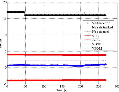
FUNCTION __________________________________________________________________________ 96 FIGURE 24:HORIZONTAL PROFILE OF SIMULATED APPROACH ______________________________________ 115 FIGURE 25:VERTICAL PROFILE OF SIMULATED APPROACH ________________________________________ 115 FIGURE 26:SET 1- IMPACT OF CONSTELLATION CHANGES ON VERTICAL POSITION ERROR (VPE) IN METERS,VPL,
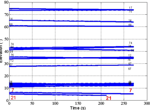
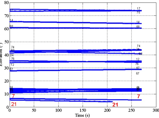
VDOP AND VFOM FOR NOMINAL CONFIGURATION _________________________________________ 118 FIGURE 27:SET 1-IDS OF THE TRACKED GPS AND GALILEO SATELLITES AS A FUNCTION OF TIME ________ 119 FIGURE 28:SET 1-ELEVATION ANGLE OF GPS AND GALILEO SATELLITES AS A FUNCTION OF TIME _______ 119 FIGURE 29:SET 1- IMPACT OF CONSTELLATION CHANGE ON HORIZONTAL POSITION ERROR (HPE) IN METERS,
HPL,HDOP AND HFOM FOR NOMINAL CONFIGURATION ____________________________________ 120 FIGURE 30:SET 2- IMPACT OF CONSTELLATION CHANGES ON VERTICAL POSITION ERROR (VPE) IN METERS,VPL,
VDOP AND VFOM FOR NOMINAL CONFIGURATION _________________________________________ 121 FIGURE 31:SET 2-IDS OF THE TRACKED GPS AND GALILEO SATELLITES AS A FUNCTION OF TIME ________ 121 FIGURE 32:SET 2-ELEVATION ANGLE OF GPS AND GALILEO SATELLITES AS A FUNCTION OF TIME _______ 122 FIGURE 33:SET 2- IMPACT OF CONSTELLATION CHANGE ON HORIZONTAL POSITION ERROR (HPE) IN METERS,
HPL,HDOP AND HFOM FOR NOMINAL CONFIGURATION ____________________________________ 122 FIGURE 34:HISTOGRAM OF THE ESTIMATED MEAN OF VPE OVER ALL SIMULATION RUNS FOR THE COMPLETE
APPROACHES IN NOMINAL CONFIGURATION _______________________________________________ 123 FIGURE 35:HISTOGRAM OF ESTIMATED STANDARD DEVIATION OF VPE OVER ALL SIMULATION RUNS FOR THE
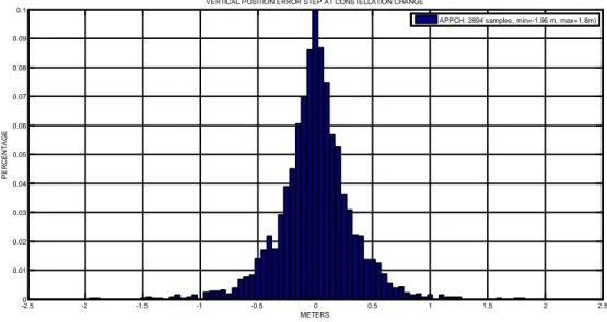
COMPLETE APPROACHES IN NOMINAL CONFIGURATION _______________________________________ 123 FIGURE 36:HISTOGRAM OF VPE STEPS AT CONSTELLATION CHANGE OVER ALL SIMULATION RUNS FOR THE
COMPLETE APPROACHES IN NOMINAL CONFIGURATION _______________________________________ 124 FIGURE 37:HISTOGRAM OF VPL STEPS AT CONSTELLATION CHANGE OVER ALL SIMULATION RUNS FOR THE
COMPLETE APPROACHES IN NOMINAL CONFIGURATION _______________________________________ 124 FIGURE 38:COMPARISON OF THE HISTOGRAMS OF THE ESTIMATED MEAN OF VPE OVER ALL SIMULATION RUNS
BEFORE AND AFTER THE FAF IN NOMINAL CONFIGURATION ___________________________________ 125 FIGURE 39:COMPARISON OF THE HISTOGRAMS OF ESTIMATED STANDARD DEVIATION OF VPE OVER ALL
FIGURE 41:HISTOGRAM OF VPL STEPS AT CONSTELLATION CHANGE OVER ALL SIMULATION RUNS BEFORE AND AFTER THE FAF IN NOMINAL CONFIGURATION _____________________________________________ 128 FIGURE 42:SET 1– IMPACT OF CONSTELLATION CHANGES ON VERTICAL POSITION ERROR (VPE) IN METERS,VPL,
VDOP AND VFOM WITH CONSTELLATION FREEZING ALGORITHM ______________________________ 129 FIGURE 43:SET 1-IDS OF TRACKED GPS AND GALILEO SATELLITES AS A FUNCTION OF TIME ____________ 129 FIGURE 44:SET 1-ELEVATION ANGLE OF GPS AND GALILEO SATELLITES AS A FUNCTION OF TIME _______ 130 FIGURE 45:SET 1– IMPACT OF CONSTELLATION CHANGES ON HORIZONTAL POSITION ERROR (HPE) IN METERS,
HPL,HDOP AND HFOM WITH CONSTELLATION FREEZING ALGORITHM _________________________ 131 FIGURE 46:SET 2– IMPACT OF CONSTELLATION CHANGES ON VERTICAL POSITION ERROR (VPE) IN METERS,VPL,
VDOP,VFOM WITH CONSTELLATION FREEZING ALGORITHM _________________________________ 132
FIGURE 47:IDS OF TRACKED GPS AND GALILEO SATELLITES AS A FUNCTION OF TIME __________________ 132 FIGURE 48:ELEVATION ANGLE OF GPS AND GALILEO SATELLITES AS A FUNCTION OF TIME _____________ 133 FIGURE 49:SET 2– IMPACT OF CONSTELLATION CHANGES ON HORIZONTAL POSITION ERROR (HPE) IN METERS,
HPL,HDOP AND HFOM WITH CONSTELLATION FREEZING ALGORITHM _________________________ 133 FIGURE 50:HISTOGRAM OF ESTIMATED MEAN OF VPE OVER ALL SIMULATION RUNS FOR THE COMPLETE
APPROACHES _______________________________________________________________________ 134 FIGURE 51:HISTOGRAM OF ESTIMATED STD OF VPE OVER ALL SIMULATION RUNS FOR THE COMPLETE
APPROACHES _______________________________________________________________________ 135 FIGURE 52:HISTOGRAM OF VPE STEPS AT CONSTELLATION CHANGE OVER ALL SIMULATION RUNS FOR THE
COMPLETE APPROACHES ______________________________________________________________ 135 FIGURE 53:HISTOGRAM OF VPL STEPS AT CONSTELLATION CHANGE OVER ALL SIMULATION RUNS FOR THE
COMPLETE APPROACHES ______________________________________________________________ 136 FIGURE 54:COMPARISON OF THE HISTOGRAMS OF ESTIMATED MEAN OF VPE OVER ALL SIMULATION RUNS BEFORE AND AFTER THE FAF WITH CONSTELLATION FREEZING ALGORITHM _____________________________ 137 FIGURE 55:COMPARISON OF HISTOGRAMS OF ESTIMATED STD OF VPE OVER ALL SIMULATION RUNS BEFORE AND
AFTER THE FAF WITH CONSTELLATION FREEZING ALGORITHM _________________________________ 138 FIGURE 56:GBAS CERTIFICATION MODEL [MURPHY,2005] _____________________________________ 144 FIGURE 57:GBASNSE GENERATOR [MURPHY,2005] __________________________________________ 144 FIGURE 58:CURVE FIT TO 𝝈𝒙𝒕𝒑𝒌𝝈𝒗𝒑𝒑𝒕 VS 𝝈𝒗𝒑𝒑𝒕DISTRIBUTION [MURPHY,2009] ___________________ 148 FIGURE 59:STUDY OF THE IMPACT OF THE CORRELATION ALGORITHM [MURPHY,2009] ________________ 149 FIGURE 60:CORRELATION COEFFICIENT DISTRIBUTION COMPARISON [MURPHY,2009] _________________ 150 FIGURE 61:GBASNSE STEP GENERATOR [MURPHY,2009] ______________________________________ 150 FIGURE 62: OBSERVED 𝝈𝒗𝒑𝒑𝒕 HISTOGRAM SUPERIMPOSED FOR ALL AIRPORTS FOR GAST-C AND GADB3 USING
SAME PROBABILITIES AS IN [MURPHY,2009] _____________________________________________ 168 FIGURE 63:COMPARISON BETWEEN OBSERVED 𝝈𝒗𝒑𝒑𝒕CDF FOR ALL SIMULATED AIRPORTS FOR GAST-C AND
GADB3 AND KVERT GENERATION FUNCTION FROM [MURPHY,2005] _________________________ 168 FIGURE 64:KVERT GENERATION FUNCTION FROM [MURPHY,2005] _______________________________ 168 FIGURE 65: OBSERVED 𝝈𝒗𝒑𝒑𝒕 HISTOGRAMS SUPERIMPOSED FOR ALL AIRPORTS FOR GAST-C AND GADB3 USING
DO-245A PROBABILITIES _____________________________________________________________ 169
FIGURE 66: OBSERVED 𝝈𝒗𝒑𝒑𝒕CDF FOR ALL AIRPORTS FOR GAST-C AND GADB3 USING DO-245A
PROBABILITIES _____________________________________________________________________ 169 FIGURE 67: OBSERVED 𝝈𝒗𝒑𝒑𝒕 HISTOGRAMS SUPERIMPOSED FOR HIGH LATITUDES AIRPORTS FOR GAST-C AND
GADB3 __________________________________________________________________________ 169
FIGURE 68: OBSERVED 𝝈𝒗𝒑𝒑𝒕CDF SUPERIMPOSED FOR HIGH LATITUDES AIRPORTS FOR GAST-C AND GADB3 _________________________________________________________________________________ 169 FIGURE 69: OBSERVED 𝝈𝒗𝒑𝒑𝒕 HISTOGRAM S FOR GAST-C AND GADB3 _____________________________ 170 FIGURE 70:COMPARISON BETWEEN OBSERVED 𝝈𝒗𝒑𝒑𝒕CDF FOR GAST-C AND GADB3 AND KVERT GENERATION FUNCTION FROM [MURPHY,2005] _____________________________________________________ 170 FIGURE 71:𝝈𝒘𝒉𝒑𝒑CDF SUPERIMPOSED FOR ALL AIRPORTS FOR GAST-C AND GADB3 ________________ 172 FIGURE 72:𝝈𝒎𝒊𝒏CDF SUPERIMPOSED FOR ALL AIRPORTS FOR GAST-C AND GAD B3 _________________ 172
FIGURE 74: HISTOGRAM OF𝜶 = 𝝈𝒘𝒉𝒑𝒑/𝝈𝒗𝒑𝒑𝒕 SUPERIMPOSED FOR ALL AIRPORTS ____________________ 172 FIGURE 75:CORRELATION COEFFICIENT BETWEEN VERTICAL AND WORST HORIZONTAL ERRORS ___________ 173 FIGURE 76 AND 77:COMPARISON OF THE CORRELATION COEFFICIENT OF TWO SEQUENCES BEFORE AND AFTER
GEOMETRICAL CORRELATION __________________________________________________________ 174 FIGURE 78:𝝈𝒘𝒉𝒑𝒑 HISTOGRAM FOR HIGH LATITUDES SUPERIMPOSED FOR GAST-C AND GASB3 _________ 174 FIGURE 79:𝝈𝒘𝒉𝒑𝒑CDF FOR HIGH LATITUDES SUPERIMPOSED FOR GAST-C AND GASB3 ______________ 174 FIGURE 80:OBSERVED 𝝈𝒘𝒉𝒑𝒑 HISTOGRAM FOR GAST-C AND GAD-B3 ____________________________ 175 FIGURE 81:COMPARISON BETWEEN OBSERVED 𝝈𝒘𝒉𝒑𝒑CDF FOR GAST-C AND GADB3 AND
𝑲𝒙𝒕𝒑𝒌 GENERATION FUNCTION FROM [MURPHY,2005] ____________________________________ 175
FIGURE 82:OBSERVED NOMINAL 𝝈𝒗𝒑𝒑𝒕𝒔𝒕𝒑𝒑 DISTRIBUTION FOR GAST-C AND GADB3 USING ENAC MEAN PROBABILITIES _____________________________________________________________________ 178 FIGURE 83:COMPARISON BETWEEN OBSERVED NOMINAL 𝝈𝒗𝒑𝒑𝒕𝒔𝒕𝒑𝒑CDF FOR GAST-C AND GADB3 AND
𝑲𝒗𝒑𝒑𝒕𝒔𝒕𝒑𝒑 GENERATION FUNCTION FROM [MURPHY,2009] ________________________________ 178
FIGURE 84: NOMINAL 𝝈𝒘𝒉𝒑𝒑𝒔𝒕𝒑𝒑 HISTOGRAM FOR ALL AIRPORTS FOR GAST-C AND GAD-B3 USING ENAC
MEAN PROBABILITIES ________________________________________________________________ 179 FIGURE 85:COMPARISON BETWEEN OBSERVED NOMINAL 𝝈𝒘𝒉𝒑𝒑𝒔𝒕𝒑𝒑CDF FOR GAST-C USING ENAC MEAN
PROBABILITIES AND GADB3 AND 𝑲𝒙𝒕𝒑𝒌𝒔𝒕𝒑𝒑 GENERATION FUNCTION FROM [MURPHY,2009] _____ 179 FIGURE 86:OBSERVED FAULTED 𝝈𝒗𝒑𝒑𝒕𝒔𝒕𝒑𝒑 DISTRIBUTION FOR GAST-C AND GADB3 USING ENAC MEAN
PROBABILITIES _____________________________________________________________________ 180 FIGURE 87:COMPARISON BETWEEN OBSERVED FAULTED 𝝈𝒗𝒑𝒑𝒕𝒔𝒕𝒑𝒑CDF FOR GAST-C AND GADB3 AND
𝑲𝒗𝒑𝒑𝒕𝒔𝒕𝒑𝒑 GENERATION FUNCTION FROM [MURPHY,2009] ________________________________ 180
FIGURE 88:OBSERVED FAULTED 𝝈𝒘𝒉𝒑𝒑𝒔𝒕𝒑𝒑 DISTRIBUTION FOR GAST-C AND GADB3 _______________ 180 FIGURE 89:COMPARISON BETWEEN OBSERVED FAULTED 𝝈𝒘𝒉𝒑𝒑𝒔𝒕𝒑𝒑CDF FOR GAST-C AND GADB3 USING
ENAC MEAN PROBABILITIES AND 𝑲𝒙𝒕𝒑𝒌𝒔𝒕𝒑𝒑 GENERATION FUNCTION FROM [MURPHY,2009] _____ 180 FIGURE 90:OBSERVED 𝝈𝒗𝒑𝒑𝒕 HISTOGRAM FOR GAST-D AND GADB3 USING ENAC MEAN PROBABILITIES _ 182 FIGURE 91:COMPARISON BETWEEN OBSERVED 𝝈𝒗𝒑𝒑𝒕CDF FOR GAST-D/GADB3 USING ENAC MEAN
PROBABILITIES AND 𝑲𝒗𝒑𝒑𝒕 GENERATION FUNCTION FROM [MURPHY ET AL.,2009] FOR GAST-D _____ 182 FIGURE 92:OBSERVED 𝝈𝒘𝒉𝒑𝒑 HISTOGRAM FOR GAST-D AND GADB3 USING ENAC MEAN PROBABILITIES 182 FIGURE 93:COMPARISON BETWEEN OBSERVED 𝝈𝒘𝒉𝒑𝒑CDF FOR GAST-D/GADB3 USING ENAC MEAN
PROBABILITIES AND 𝑲𝒙𝒕𝒑𝒌 GENERATION FUNCTION FROM [MURPHY ET AL.,2009] ________________ 182 FIGURE 94:OBSERVED NOMINAL 𝝈𝒔𝒕𝒑𝒑_𝒗𝒑𝒑𝒕 DISTRIBUTION FOR GAST-D AND GADB3 USING ENAC MEAN
PROBABILITIES _____________________________________________________________________ 183 FIGURE 95:COMPARISON BETWEEN OBSERVED NOMINAL 𝝈𝒗𝒑𝒑𝒕𝒔𝒕𝒑𝒑CDF FOR GAST-D AND GADB3 AND
𝑲𝒗𝒑𝒑𝒕𝒔𝒕𝒑𝒑 GENERATION FUNCTION FROM [MURPHY ET AL.,2009] FOR GAST-D __________________ 183
FIGURE 96:OBSERVED NOMINAL 𝝈𝒘𝒉𝒑𝒑𝒔𝒕𝒑𝒑 DISTRIBUTION FOR GAST-D AND GADB3 USING ENAC MEAN PROBABILITIES _____________________________________________________________________ 183 FIGURE 97:COMPARISON BETWEEN OBSERVED NOMINAL 𝝈𝒘𝒉𝒑𝒑𝒔𝒕𝒑𝒑CDF FOR GAST-D AND GADB3 USING
ENAC MEAN PROBABILITIES AND 𝑲𝒙𝒕𝒑𝒌𝒔𝒕𝒑𝒑 GENERATION FUNCTION FROM [MURPHY ET AL.,2009] FOR
GAST-D __________________________________________________________________________ 183 FIGURE 98:OBSERVED FAULTED 𝝈𝒗𝒑𝒑𝒕𝒔𝒕𝒑𝒑 DISTRIBUTION FOR GAST-D AND GADB3 USING ENAC MEAN
PROBABILITIES _____________________________________________________________________ 184 FIGURE 99:COMPARISON BETWEEN OBSERVED FAULTED 𝝈𝒗𝒑𝒑𝒕𝒔𝒕𝒑𝒑CDF FOR GAST-D AND GADB3 AND
𝑲𝒗𝒑𝒑𝒕𝒔𝒕𝒑𝒑 GENERATION FUNCTION FROM [MURPHY ET AL.,2009] FOR GAST-D __________________ 184
FIGURE 100:OBSERVED FAULTED 𝝈𝒘𝒉𝒑𝒑𝒔𝒕𝒑𝒑 DISTRIBUTION FOR GAST-D AND GADB3 USING ENAC MEAN PROBABILITIES _____________________________________________________________________ 184 FIGURE 101:COMPARISON BETWEEN OBSERVED FAULTED 𝝈𝒘𝒉𝒑𝒑𝒔𝒕𝒑𝒑CDF FOR GAST-D AND GADB3 USING
ENAC MEAN PROBABILITIES AND 𝑲𝒙𝒕𝒑𝒌𝒔𝒕𝒑𝒑 GENERATION FUNCTION FROM [MURPHY ET AL.,2009] FOR
GAST-D __________________________________________________________________________ 184 FIGURE 102:CLASSICAL RECEIVER ARCHITECTURE ______________________________________________ 223
TABLE 1:DECISION HEIGHTS AND VISUAL REQUIREMENTS [ICAO,2001] _____________________________ 27 TABLE 2:SIS PERFORMANCE REQUIREMENTS [ICAO,2006] ________________________________________ 31 TABLE 3:ALERT LIMITS ASSOCIATED TO TYPICAL OPERATIONS [ICAO,2006] __________________________ 32 TABLE 4:GNSS SIGNALS FOR CIVIL AVIATION __________________________________________________ 39 TABLE 5:KLOBUCHAR ALGORITHM [ARINC,2004] ______________________________________________ 62 TABLE 6:AVERAGE METEOROLOGICAL PARAMETERS FOR TROPOSPHERIC DELAY [RTCA,2006] ___________ 63 TABLE 7:SEASONAL VARIATION OF METEOROLOGICAL PARAMETERS FOR TROPOSPHERIC DELAY [RTCA,2006] 64 TABLE 8:PARAMETERS FOR THE ALLAN VARIANCE OF SEVERAL OSCILLATORS [WINKEL,2000] ___________ 66 TABLE 9:PARAMETERS FOR DLL TRACKING ERROR VARIANCE COMPUTATION _________________________ 75 TABLE 10:NON-AIRCRAFT ELEMENTS ACCURACY REQUIREMENT [RTCA,2004] _______________________ 81 TABLE 11:AIRBORNE ACCURACY DESIGNATOR [RTCA,2004] _____________________________________ 81 TABLE 12:AIRFRAME MULTIPATH DESIGNATOR [RTCA,2004] _____________________________________ 82 TABLE 13:RESIDUAL IONOSPHERIC UNCERTAINTY PARAMETERS ASSUMPTIONS [RTCA,2004] ____________ 83 TABLE 14:YUMA ALMANACS PARAMETERS____________________________________________________ 91 TABLE 15:EPHEMERIS EQUATIONS [ARINC,2004] ______________________________________________ 92 TABLE 16:EPHEMERIS VELOCITY EQUATIONS __________________________________________________ 93 TABLE 17:AIRPORT LOCATION FOR GPS-GALILEO AND RAIM SIMULATIONS ________________________ 116 TABLE 18:MINIMUM AND MAXIMUM ESTIMATED MEAN VPE OBSERVED IN NOMINAL CONFIGURATION ______ 125 TABLE 19:MINIMUM AND MAXIMUM ESTIMATED VPE STANDARD DEVIATION OBSERVED IN NOMINAL
CONFIGURATION ____________________________________________________________________ 126 TABLE 20:MINIMUM AND MAXIMUM ESTIMATED VPE STEPS OBSERVED IN NOMINAL CONFIGURATION ______ 127 TABLE 21:MINIMUM AND MAXIMUM ESTIMATED VPL STEPS OBSERVED IN NOMINAL CONFIGURATION ______ 128 TABLE 22:MINIMUM AND MAXIMUM ESTIMATED MEAN VPE OBSERVED WITH CONSTELLATION FREEZING
ALGORITHM ________________________________________________________________________ 137 TABLE 23:MINIMUM AND MAXIMUM ESTIMATED MEAN VPE OBSERVED WITH CONSTELLATION FREEZING
ALGORITHM ________________________________________________________________________ 138 TABLE 24:𝑲𝒙𝒕𝒑𝒌 CANDIDATES_____________________________________________________________ 148 TABLE 25:PROBABILITY OF STEP EVENTS DURING EXPOSURE INTERVALS [MURPHY,2009] ______________ 152 TABLE 26:CONSTELLATION STATE PROBABILITIES ______________________________________________ 163 TABLE 27:AIRPORT LOCATIONS ____________________________________________________________ 167 TABLE 28: RISE/SET PROBABILITIES __________________________________________________________ 178 TABLE 29:BPSK SIMULATION PLAN _________________________________________________________ 236 TABLE 30:BPSK SIMULATION PLAN _________________________________________________________ 236 TABLE 31:BPSK SIMULATION PLAN _________________________________________________________ 236 TABLE 32:BPSK VALIDATION RESULTS (𝑩 = 𝟒𝑴𝑯𝒛,𝑻𝑫𝑳𝑳 = 𝟎. 𝟎𝟎𝟏𝒔,𝑻𝑷𝑳𝑳 = 𝟎. 𝟎𝟎𝟏𝒔) _____________ 237 TABLE 33:BPSK VALIDATION RESULTS (𝑩 = 𝟒𝑴𝑯𝒛,𝑻𝑫𝑳𝑳 = 𝟎. 𝟎𝟐𝟎𝒔,𝑻𝑷𝑳𝑳 = 𝟎. 𝟎𝟐𝟎𝒔) _____________ 238 TABLE 34:BPSK VALIDATION RESULTS (𝑩 = 𝟒𝑴𝑯𝒛,𝑻𝑫𝑳𝑳 = 𝟎. 𝟎𝟎𝟏𝒔,𝑻𝑷𝑳𝑳 = 𝟎. 𝟎𝟎𝟏𝒔) _____________ 239 TABLE 35:BOC(1,1) VALIDATION RESULTS (𝑩 = 𝟒𝑴𝑯𝒛,𝑻𝑫𝑳𝑳 = 𝟎. 𝟎𝟎𝟏𝒔,𝑻𝑷𝑳𝑳 = 𝟎. 𝟎𝟎𝟏𝒔) __________ 240 TABLE 36:BOC(1,1) VALIDATION RESULTS (𝑩 = 𝟒𝑴𝑯𝒛,𝑻𝑫𝑳𝑳 = 𝟎. 𝟏𝟎𝟎𝒔,𝑻𝑷𝑳𝑳 = 𝟎. 𝟎𝟐𝟎𝒔) __________ 241 TABLE 37:BOC(1,1) VALIDATION RESULTS (𝑩 = 𝟏𝟎𝑴𝑯𝒛,𝑻𝑫𝑳𝑳 = 𝟎. 𝟏𝟎𝟎𝒔,𝑻𝑷𝑳𝑳 = 𝟎. 𝟎𝟐𝟎𝒔) ________ 242 TABLE 38:CBOC VALIDATION RESULTS (𝑪𝑺 = 𝟏𝟏𝟐𝒄𝒉𝒊𝒑,𝑻𝑫𝑳𝑳 = 𝟎. 𝟏𝟎𝟎𝒔,𝑻𝑷𝑳𝑳 = 𝟎. 𝟎𝟐𝟎𝒔) _________ 243 TABLE 39:CBOC VALIDATION RESULTS (𝑪𝑺 = 𝟏𝟏𝟐𝒄𝒉𝒊𝒑,𝑻𝑫𝑳𝑳 = 𝟎. 𝟎𝟎𝟏𝒔,𝑻𝑷𝑳𝑳 = 𝟎. 𝟎𝟎𝟏𝒔) _________ 244
1.
Chapter 1: Introduction
1.1 Motivation
Since many years, civil aviation has identified GNSS as an attractive mean to provide navigation services. In fact, in recent years, GNSS slowly became one of the reference mean of navigation for civil aviation users due to its wide coverage area. Since a majority of commercial aircraft is now equipped with GNSS receivers, aeronautical rules have evolved so as to switch from classical radionavigation to RNAV or Area Navigation in order to be less dependent from ground facilities.
This evolution was possible using the US Global Positioning System which currently broadcasts in particular the GPS L1 C/A signal. This signal is of particular interest for civil aviation since it is emitted in an Aeronautical Radio Navigation Services (ARNS) band which is reserved for aeronautical applications and protected from interferences.
However, since civil aviation requirements can be very stringent in terms of accuracy, integrity, availability and continuity, GPS standalone receivers cannot be used as a sole mean of navigation. This fact has led the ICAO to define and develop standard augmentation systems to correct the GPS L1 C/A and to monitor the quality of the received Signal-In-Space (SIS). Different solutions exist depending on where and how the augmentation is implemented. We can distinguish SBAS (Satellite Based Augmentation Systems), GBAS (Ground Based Augmentation Systems), ABAS (Aircraft Based Augmentation Systems). Each system can allow fulfilling applicable SIS requirements up to a certain level. Two types of ABAS systems can be distinguished: Receiver Autonomous Integrity Monitoring (RAIM) when only GNSS information is used, Aircraft Autonomous Integrity Monitoring (AAIM) when information from other on-board sensors is also used. It is important to notice that GBAS and SBAS provide the possibility to correct GPS L1 C/A signal pseudorange measurements by transmitting adequate corrections to the receivers as well as monitoring the integrity of the signal. On the other hand, ABAS mainly permits to monitor the integrity of GPS L1 C/A. In addition, improvements of the accuracy, availability and continuity of the position can be obtained in the case of AAIM thanks to the integration in the position solution of external sensors measurements.
In fact, the most demanding phases of flight in terms of SIS performance are the approaches which have been categorized by the ICAO as following:
• Non precision approaches (NPA)
• Approaches with vertical guidance (APV)
• Precision approaches (CAT I, CAT II, CAT III a/b/c)
Current GNSS standards published by ICAO cover every phase of flight from Oceanic down to CAT I precision approaches thanks to GBAS. The aim of this study is to investigate and characterize the behaviour of the position error of promising positioning solutions for civil aviation users in the context of the on-going development of new GNSS constellations as well as new GNSS signals. In fact, during approaches and in particular precision approaches, the behaviour of the GNSS NSE (Navigation Sensor Error) has to be precisely known so that autoland guidance laws can be adapted to anticipate and cancel the impact of undesired or spurious position errors.
Airbus as an aircraft manufacturer is particularly interested in increasing its knowledge of the impact of the different errors affecting pseudorange measurements on the NSE and in evaluating the benefits
brought by future evolutions of the GNSS systems which is why a partnership was created between Airbus and ENAC to investigate these subjects and which resulted in the co-funding of this PhD.
In this context, we decided to focus our attention on two promising position solutions which are GPS L1 C/A and GBAS as well as GPS/GALILEO and RAIM.
It was felt that no software models were already available for GPS L1 C/A and GBAS and GPS/GALILEO and RAIM and suited to the needs of Airbus and in particular the needs for evolution of the models, and the need to increase the knowledge through participation to the development.
GBAS is composed of two main elements:
• The ground station which includes an active VDB (VHF Broadcast) transmitter and several reference receivers which location is precisely known. This station is able to compute differential pseudorange corrections and to monitor the quality of the GPS SIS.
• The airborne receiver which includes the capability to receive and process the GBAS SIS in addition to GPS SIS. Using the data sent by the ground station, the user receiver is able to correct its own measurements but also to exclude some of them and to compute protection levels which are an evaluation of the confidence that the user can have in the final position solution.
GBAS is currently foreseen as an important source of innovation for civil aviation since it has already been certified for CAT-I precision approaches and may allow reaching ICAO requirements down to CAT-II/III minima, then providing an alternative to classical landing system ILS. This possibility is actively investigated and ICAO and Industry standardization bodies are currently deriving requirements for GBAS CAT II-III.
However, mandatory regulations for the certification of CAT II/III Autoland capability of a navigation mean require numerous simulations to assess statistically the aircraft capability to autoland. Therefore, it is necessary to identify the GBAS GLS (GPS Landing System) behaviour with sufficient fidelity, taking into account errors affecting the SIS performance. The outcomes of these simulations are intended to feed an autoland simulator dedicated to airworthiness assessment of aircraft guidance laws.
A model has previously been proposed in the past for CAT I GBAS autoland simulations but the evolution of CAT II/III requirements and the lack of information on the validation process used made it necessary to analyze and improve if necessary the existing model. The aim of the study on GBAS is then to derive the rationale for the architecture of the state of the art model, to propose possible improvements and to develop necessary evolutions to extend the use of this model to CAT II/III autoland simulations. The expected outcome is then to obtain a simulation tool to be used in the frame of certification of GBAS CAT II/III.
RAIM and GPS/GALILEO is the other position solution which is studied. Today RAIM and/or AAIM are commonly used to provide integrity monitoring for phases of flight down to Non Precision Approaches using GPS L1 C/A measurements and the associated redundancy. However, current performance associated to GPS L1 C/A and GPS constellation is not sufficient to meet civil aviation requirements for more stringent phases of flight and in particular, the vertical requirements associated to APV and CAT-I.
The introduction of new signals and constellations - such as GPS L5 and GALILEO for example – will significantly increase the number of available signals and satellites, the quality of the
measurements as well as the quality of constellation geometries. Thus, RAIM may provide a simple mean to monitor the quality of the SIS and to reach more stringent phases of flights such as APV or CAT-I operations.
This possibility has been investigated by civil aviation community during recent years as in [MARTINEAU, 2008], [LEE, 2007] and [WALTER, 2008]. RAIM is now foreseen as an interesting candidate to provide integrity monitoring for CAT-I. Different algorithms have been studied and their performance in terms of availability has been published. It results that RAIM alone does not seem to provide sufficient protection for CAT-I approaches. New possibilities to extend RAIM to APV and CAT-I are under study and it can be reasonably assumed that RAIM using GPS and GALILEO constellations could be used in the near future (Advanced RAIM) [GEAS, 2010].
Therefore, it appears necessary to address the specific phenomena that will result from the combination of two different constellations in one positioning solution. The interest of this study was thus to provide a microscopic analysis of the temporal behaviour of GPS and GALILEO NSE and RAIM, for CAT-I type of operations. Indeed, the use of different types of satellites, the constellation changes, potential loss of frequencies may imply unexpected behaviour of NSE. The impact of the introduction of this new positioning solution has to be investigated so as to limit unwanted effects for aircraft flight control systems which use the GNSS computed position. A particular attention has been paid to constellation changes. So as to make this study possible, a GPS/GALILEO and RAIM receiver model has been developed.
1.2 Original Contribution
This section gives a brief insight in the original contributions obtained thanks to this study. Each point is extensively described all along this document:
• Development of a GNSS receiver simulator including multi-constellation and multi-frequency position solution.
• Study of the temporal behaviour of GPS/GALILEO and LSR RAIM NSE and assessment of the impact of constellation changes.
• Design of an algorithm to prevent the impact of constellation changes on GPS/GALILEO and LSR RAIM position solution during final approaches.
• Analysis of a state of the art GBAS GAST-C NSE model for GBAS CAT-I autoland simulations
• Proposal of an alternate model for GBAS CAT-I autoland simulations
• Proposal of a GBAS GAST-D NSE model for GBAS CAT-II/III based on the previous so as to reflect evolution of civil aviation requirements concerning GBAS GAST-D service.
1.3 Dissertation organization
The following report is organized as follows.
First, Chapter 2 gives an overview of requirements applicable to GNSS use for navigation of civil aviation aircraft. It describes the different categories of phases of flight with an emphasis on approaches. The concept of Performance Based Navigation (PBN) is then introduced. The operational criteria of ICAO for GNSS based navigation are defined and the associated Signal In Space requirements are reminded for each phase of flight. Finally, a review of the different categories of GNSS receivers classified by RTCA and agreed by EUROCAE is presented which is followed by the presentation of initial studies led by EUROCAE on possible multi-constellation multi-signals GNSS receivers.
The state of the art of GNSS signals structure and the associated signal processing is presented in Chapter 3. Thus, the different GNSS signals currently available for civil aviation or which will be operational with the introduction of new GPS signals as well as the GALILEO constellation are described. Classical architectures of the signal receiver for processing these signals are then given.
The purpose of Chapter 4 is to highlight the different pseudorange measurement models considered in this study as well as the receiver simulator developed and used to derive the results obtained in the course of this work. First, models used to represent the errors affecting the pseudorange measurements are developed. Then, the pseudorange measurement error models applicable to civil aviation GNSS receivers for position computation are reminded in the case of RAIM and GPS/GALILEO and GBAS GAST-C and GAST-D with GPS L1 C/A. The next sections present the architecture and the implementation of the multi-constellation and multi-signal GNSS receiver simulator which includes in particular the receiver signal processing, the position computation as well as the integrity monitoring.
Chapter 5 gathers the results obtained during simulation concerning the RAIM and GPS/GALILEO combination model and more precisely the behaviour of the NSE as well as the impact of constellation changes on this NSE.
Chapter 6 presents the outcomes of our study on a GBAS GAST-D NSE model for CAT II/III autoland simulations. This chapter thus addresses a review and a mathematical analysis of an existing GBAS GAST-C NSE model for CAT-I autoland simulations. It then presents our proposal of an equivalent GBAS GAST-C NSE model for CAT-I autoland simulations which takes into account the conclusions derived from the simulation run in the frame of this study. The proposed model is moreover enhanced so as to provide a solution for simulating GBAS GAST-D NSE for CAT II/III autoland simulations by taking into account recent evolutions of GBAS CAT II/III standards.
2.
Chapter 2: Civil Aviation Requirements
2.1 CIVIL AVIATION AUTHORITIES ... 23
2.1.1 International Civil Aviation Organization (OACI) ... 23 2.1.2 RTCA, Inc. ... 23 2.1.3 EUROCAE... 24 2.1.4 FAA and EASA ... 24
2.2 PHASES OF FLIGHT ... 24
2.2.1 Categories of flight phases ... 24 2.2.2 Approaches ... 25
2.3 PERFORMANCE BASED NAVIGATION ... 27 2.4 OPERATIONAL CRITERIA FOR NAVIGATION PERFORMANCE ... 28
2.4.1 Accuracy ... 28 2.4.2 Availability ... 29 2.4.3 Continuity ... 29 2.4.4 Integrity ... 29
2.5 ANNEX 10SIGNAL IN SPACE PERFORMANCE REQUIREMENTS ... 30 2.6 EQUIPMENT CLASSES ... 33
2.6.1 Operational Classes ... 33 2.6.2 Functional Classes ... 33
2.7 COMBINED RECEIVERS ... 34 2.8 SYNTHESIS ... 35
2.1 Civil Aviation Authorities
So as to be authorized for use aboard aircraft, navigation equipments have to fulfil a number of requirements so as to ensure their capability to perform their function. The aim of this section is to briefly present and describe the main organisations which issue these requirements.
2.1.1 International Civil Aviation Organization (ICAO)
The International Civil Aviation Organization (ICAO) is the agency of the United Nations, which codifies the principles and techniques of international air navigation and fosters the planning and development of international air transport to ensure safe and orderly growth. The ICAO Council adopts standards and recommended practices (SARPs) concerning air navigation, prevention of unlawful interference, and facilitation of border-crossing procedures for international civil aviation. In addition, the ICAO defines the protocols for air accident investigation followed by transport safety authorities in countries signatory to the Convention on International Civil Aviation, commonly known as the Chicago Convention [ICAO, 2008].
In particular, The International Civil Aviation Organization (ICAO) is responsible for establishing the standards for radio navigation aids, including the ones concerning GNSS. They are mainly defined in the Annex 10 to the Convention on International Civil Aviation.
2.1.2 RTCA, Inc.
RTCA, Inc. is a private, not-for-profit Corporation that develops consensus-based recommendations regarding communications, navigation, surveillance, and air traffic management (CNS/ATM) system issues. RTCA functions as a Federal Advisory Committee. Its recommendations are used by the Federal Aviation Administration (FAA) as the basis for policy, program, and regulatory decisions and by the private sector as the basis for development, investment and other business decisions [RTCA, 2010].
In particular, the working group SC-159 of RTCA focuses on GNSS systems. His task is to develop minimum standards that form the basis for FAA approval of equipment using GPS as primary means of civil aircraft navigation.
According to [RTCA, 2006], RTCA’s objectives include but are not limited to:
• coalescing aviation system user and provider technical requirements in a manner that helps government and industry meet their mutual objectives and responsibilities;
• analysing and recommending solutions to the system technical issues that aviation faces as it continues to pursue increased safety, system capacity and efficiency;
• developing consensus on the application of pertinent technology to fulfill user and provider requirements, including development of minimum operational performance standards for electronic systems and equipment that support aviation; and
• assisting in developing the appropriate technical material upon which positions for the International Civil Aviation Organization and the International Telecommunication Union and other appropriate international organizations can be based.
Different RTCA publications have been used during this PhD the main one being:
• DO-229D – Minimum Operational Performance Standards for Global Positioning
System/Wide Area Augmentation System Airborne Equipment.
• DO-245A – Minimum Aviation System Performance Standards for Local Area Augmentation
• DO-253C – Minimum Operational Performance Standards for GPS Local Area Augmentation
System Airborne Equipment
2.1.3 EUROCAE
The European Organization for Civil Aviation Equipment (EUROCAE) is a non-profit making organization which was formed to provide a European forum for resolving technical problems with electronic equipment for air transport. EUROCAE deals exclusively with aviation standardization (Airborne and Ground Systems and Equipments) and related documents as required for use in the regulation of aviation equipment and systems [EUROCAE, 2010]. Its work programme is principally directed to the preparation of performance specifications and guidance documents for civil aviation equipment, for adoption and use at European and world-wide levels.
EUROCAE is composed of manufacturers, service providers, national and international aviation authorities as well as users (airlines, airports). EUROCAE can be considered as the equivalent of RTCA for Europe.
To develop EUROCAE documents, EUROCAE organizes Working Groups (WG). In particular, the WG-62 is responsible for the preparation of aviation use of GALILEO and the development of initial Minimum Operation Performance Specifications (MOPS) for the first generation of GALILEO airborne receivers.
The use of dual constellation receivers (GPS+GALILEO) should be standardized jointly by EUROCAE and RTCA in a future MOPS.
Now that the different organisations involved in the elaboration of the standards related to the use of GNSS systems for civil aviation have been presented, we will present the standardized phases of flight for civil aircraft flights.
2.1.4 FAA and EASA
The official authorities which publish mandatory requirements to be respected by aircraft manufacturers and airliners to fly an aircraft are the FAA and EASA. The FAA is an agency of the United States Department of Transportation. The EASA can be considered as the equivalent structure for the European Commission. Their main goal is to ensure the safety of the civil aviation air traffic.
Many of their publications are based on or refer to the standardization publications emitted by the previous organisations.
We can mention here publications which are directly related to this study and which are the airworthiness criteria for landing operations. These can be found in FAA Advisory Circular AC 120-28D [FAA, 1999] and EASA CS AWO [EASA, 2003].
2.2 Phases of Flight
2.2.1 Categories of flight phases
The flight of an aircraft consists of six major phases [CICTT, 2006]:
• Take-Off: From the application of takeoff power, through rotation and to an altitude of 35 feet above runway elevation or until gear-up selection, whichever comes first.
• Departure: From the end of the Takeoff sub-phase to the first prescribed power reduction, or until reaching 1000 feet above runway elevation or the VFR pattern (Visual Flight Rules), whichever comes first.
• Cruise: Any level flight segment after arrival at initial cruise altitude until the start of descent to the destination.
• Descent:
o Instrument Flight Rules (IFR): Descent from cruise to either Initial Approach Fix (IAF) or VFR pattern entry.
o Visual Flight Rules (VFR): Descent from cruise to the VFR pattern entry or 1000 feet above the runway elevation, whichever comes first.
• Final Approach: From the FAF (Final Approach Fix) to the beginning of the landing flare. • Landing: Transition from nose-low to nose-up attitude just before landing until touchdown. As we are particularly interested in Approaches operations we will give a more detailed description in the following section.
2.2.2 Approaches
Categories of aircraft approaches are defined according to the level of confidence that can be placed by the pilot into the system he is using to help him land the plane safely. Approaches are divided in two main segments: the aircraft first follows the indication provided by the landing system, and then the pilot takes over in the final part and controls the aircraft using visual outside information. As the reliability of the aircraft, the crew and the landing system increases, the height of the aircraft over the ground at the end of the interval of use of the information provided by the system can be decreased [MACABIAU, 1997].
Three classes of approaches and landing operation have been defined by the ICAO in the Annex 6 [ICAO, 2001] and are classified as follows:
• Non Precision Approaches and landing operations (NPA): an instrument approach and landing which utilizes lateral guidance but does not utilize vertical guidance.
• Approaches and landing operations with vertical guidance (APV): an instrument approach and landing which utilizes lateral and vertical but does not meet the requirements established for precision approach and landing operation.
• Precision approaches and landing operation: an instrument approach and landing using precision lateral and vertical guidance with minima as determined by the category of operation.
The figure below presents the different phases of flight - and in particular the different type of approaches - along with the type of GNSS augmentations which allow conducting navigation operations for civil aviation during the corresponding phase of flight.
Figure 1: Phases of flight and GNSS augmentations [MONTLOIN, 2011]
The approaches can be defined using three different operational parameters which are the Decision Height (DH), the Distance of Visibility and the Runway Visual Range (RVR). These parameters are defined as follows [CABLER, 2002]:
Decision Height (DH) is the minimal height above the runway threshold at which as missed approach procedure must be executed if the minimal visual reference required in order continuing the approach has not been established.
Distance of Visibility is the greatest distance, determined by atmospheric conditions and expressed in units of length, at which it is possible with unaided eye to see and identify, in daylight a prominent dark object, and at night a remarkable light source.
Runway Visual Range (RVR) is the maximum distance in the landing direction at which the pilot on the centre line can see the runway surface markings, runway lights, as measured at different points along the runway and in particular in the touchdown area.
Category Minimum Descent Altitude (MDA)
Minimum Descent Height (MDH) Decision Altitude (DA)
Decision Height (DH)
Visual requirements
NPA MDA ≥ 350 ft
Depending on the airport equipment APV DA ≥ 250 ft LPV 200 DH ≥ 60 m (200ft) Precision Approaches CAT – I DH ≥ 60 m (200ft) Visibility ≥ 800 m Or RVR ≥ 550 m CAT – II 30 m (100ft) ≤ DH ≤ 60 m (200ft) RVR ≥ 300 m CAT – III A 0 m ≤ DH ≤ 30 m (100ft) RVR ≥ 175m B 0 m ≤ DH ≤ 15 m (50ft) 50 m ≤ RVR ≤ 175 m C DH = 0 m RVR = 0 m
ABAS ABAS (not standardized)
SBAS
GBAS developmentUnder
En route
oceanic domesticEn route
NPA Terminal PA APV CAT I APV1 APV2 APV baro VNAV
CAT II CAT III
Surface Departure Missed approach ABAS (missed approach)
Table 1: Decision heights and Visual requirements [ICAO, 2001]
2.3 Performance Based Navigation
The Performance Based Navigation (PBN) concept specifies that aircraft RNAV system performance requirements be defined in terms of the accuracy, integrity, availability, continuity and functionality, which are needed for the proposed operations in the context of a particular airspace concept. The PBN concept represents a shift from sensor-based to performance-based navigation. Performance requirements are identified in navigation specifications, which also identify the choice of navigation sensors that may be used to meet the performance requirements. These navigation specifications are defined at a sufficient level of detail to facilitate global harmonization by providing specific implementation guidance for States and operators [ICAO, 2008].
PBN offers a number of advantages over the sensor-specific method of developing airspace and obstacle clearance criteria:
• Reduces the need to maintain sensor-specific routes and procedures, and their associated costs • Avoids the need for developing sensor-specific operations with each new evolution of
navigation systems, which would be cost-prohibitive
• Allows for more efficient use of airspace (route placement, fuel efficiency and noise abatement)
• Clarifies how RNAV systems are used
• Facilitates the operational approval process for operators by providing a limited set of navigation specifications intended for global use.
The concept of PBN relies on RNAV systems and Required Navigation Performance (RNP) procedures. Here are reminded the definitions of these key terms [ICAO, 2008]:
Area Navigation (RNAV): A method of navigation which permits aircraft operation on any desired flight path within the coverage of station-referenced navigation aids or with the limits of the capability of self-contained aids, or a combination of these.
Area Navigation Equipment: Any combination of equipment used to provide RNAV guidance. Required Navigation Performance (RNP) Systems: An area navigation system which supports on-board performance monitoring and alerting.
Required Navigation Performance (RNP): A statement of the navigation performance necessary for operation within a defined airspace.
According to [ICAO, 2008] the required navigation performance can be defined by the Total System Error (TSE) which is illustrated in Figure 2: