Compliance error compensation in robotic-based milling

HAL Id: hal-01066945

https://hal.archives-ouvertes.fr/hal-01066945

Submitted on 22 Sep 2014

HAL is a multi-disciplinary open access

archive for the deposit and dissemination of

sci-entific research documents, whether they are

pub-lished or not. The documents may come from

teaching and research institutions in France or

abroad, or from public or private research centers.

L’archive ouverte pluridisciplinaire HAL, est

destinée au dépôt et à la diffusion de documents

scientifiques de niveau recherche, publiés ou non,

émanant des établissements d’enseignement et de

recherche français ou étrangers, des laboratoires

publics ou privés.

Compliance error compensation in robotic-based milling

Alexandr Klimchik, Dmitry Bondarenko, Anatol Pashkevich, Sébastien Briot,

Benoît Furet

To cite this version:

Alexandr Klimchik, Dmitry Bondarenko, Anatol Pashkevich, Sébastien Briot, Benoît Furet.

Compli-ance error compensation in robotic-based milling. L. Ferrier, A. Bernard, O. Gusikhin, K. Madani.

Informatics in Control, Automation and Robotics, Springer, pp.197-216, 2014. �hal-01066945�

Compliance error compensation in robotic-based milling

Alexandr Klimchik1,2, Dmitry Bondarenko1,2, Anatol Pashkevich1,2, Sébastien Briot2, Benoît Furet2,3

1

Ecole des Mines de Nantes, 4 rue Alfred-Kastler, 44307 Nantes, France 2_{Institut de Recherches en Communications et Cybernétique de Nantes, France}

3

Université de Nantes, quai de Tourville, 44035 Nantes, France {alexandr.klimchik, anatol.pashkevich}@mines-nantes.fr, {dmitry.bondarenko, sebastien.briot,

benoit.furet}@irccyn.ec-nantes.fr

Abstract. The paper deals with the problem of compliance errors compensation

in robotic-based milling. Contrary to previous works that assume that the forces/torques generated by the manufacturing process are constant, the interac-tion between the milling tool and the workpiece is modeled in details. It takes into account the tool geometry, the number of teeth, the feed rate, the spindle rotation speed and the properties of the material to be processed. Due to high level of the disturbing forces/torques, the developed compensation technique is based on the non-linear stiffness model that allows us to modify the target tra-jectory taking into account nonlinearities and to avoid the chattering effect. Illu-strative example is presented that deals with robotic-based milling of aluminum alloy.

Keywords. Industrial robot, milling, compliance error compensation, dynamic

machining force model, non-linear stiffness model.

1

Introduction

Currently, robots become more and more popular for a variety of technological processes, including high-speed precision machining. For this process, external load-ing caused by the machinload-ing force is applied on the robot tool. This force is generated by the interaction between the tool mounted on the robot end-effector and the work-piece during the material removal [1]. It is a contact force and it is distributed along the affected area of the tool cutting part. To evaluate the influence and to analyze the robot behavior while machining, the cutting force should be defined either experimen-tally or using accurate mathematical model.

To evaluate the force caused by interaction between the tool and the workpiece, two approaches can be used. The static approach allows computing the average cut-ting force without any consideration of dynamic aspect in machining system. This force serves as an external loading of the robot. This approach is widely used in anal-ysis of conventional machining processes using CNC machines [2], where the stiff-ness is high. In contrast, robots have relatively low structural stiffstiff-ness. For this

rea-son, in the case of robotic-based machining, an additional source of dynamic dis-placements of the end-effector with respect to the desired trajectory induced by robot compliance may arise. Such behavior leads to the variable contact between the ma-chining tool and the workpiece. Thus, the generated contact force depends on the current position of the robot end-effector on the trajectory. Consequently, the cutting force cannot be evaluated correctly using the static approach. In this case, the dynam-ic approach, whdynam-ich will be used in the paper, is required. It is based on computing of the force at each instant of machining process that defines loading of the robot for the next instant of processing. As a result, the dynamic aspect of robot motion under such variable cutting force can be examined for whole process.

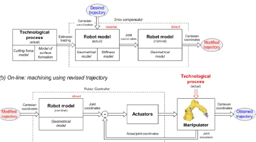
Usually, in the robot-based machining this force causes essential deflections that decrease the quality of the final product. The problem of the robot error compensation can be solved in two ways that differ in degree of modification of the robot control software:

(a) by modification of the manipulator model, which better suits to the real ma-nipulator and is used by the robot controller (in simple case, it can be limited by tun-ing of the nominal manipulator model, but may also involve essential model en-hancement by introducing additional parameters, if it is allowed by a robot manufac-turer);

(b) by modification of the robot control program that defines the prescribed tra-jectory in Cartesian space (here, using relevant error model, the input tratra-jectory is generated in such way that under the loading the output trajectory coincides with the desired one, while input trajectory differs from the target one).

Moreover, with regard to the robot-based machining, there is a solution that does not require force/torque measurements or computations [1], where the target trajecto-ry for the robot controller is modified by applying the "mirror" technique. An evident advantage of this technique is its applicability to the compensation of all types of the robot errors, including geometrical and compliance ones. However, this approach requires carrying out additional preliminary experiments which are quite expensive. So, it is suitable for the large-scale production only. Another compensation methodol-ogy has been proposed by Eastwood and Webb [3] that was used for gravitational deflection compensation for hybrid parallel kinematic machines.

This paper focuses on the modification of control program that is considered to be more realistic in practice. This approach requires also accurate stiffness model of the manipulator. From point of view of stiffness analysis, the external and forces directly influence on the manipulator equilibrium configuration and, accordingly, may modify the stiffness properties. So, they must be undoubtedly taken into account while devel-oping the stiffness model. However, in most of the related works the Cartesian stiff-ness matrix has been computed for the nominal configuration [4-5]. Such approach is suitable for the case of small deflections only. For the opposite case, the most impor-tant results have been obtained in [6-8], which deal with the stiffness analysis of ma-nipulators under the end-point loading.

Thus, to compensate errors caused by the machining process, it is required to have an accurate stiffness model and precise cutting force model. In contrast to the pre-vious works, the compliance error compensation technique presented in this work is

based on the non-linear stiffness model of the manipulator [7] and dynamic model of technological process that generates the cutting force.

2

Problem statement

For the compliance errors, the compensation technique must rely on two compo-nents. The first of them describes distribution of the stiffness properties throughout the workspace and is defined by the stiffness matrix as a function of the joint coordi-nates. The second component describes the forces/torques acting on the end-effector while the manipulator is performing its machining task (manipulator loading).

The stiffness matrix required for the compliance errors compensation highly de-pends on the robot configuration and essentially varies throughout the workspace. From general point of view, full-scale compensation of the compliance errors requires essential revision of the manipulator model embedded in the robot controller. In fact, instead of conventional geometrical model that provides inverse/direct coordinate transformations from the joint to Cartesian spaces and vice versa, here it is necessary to employ the so-called kinetostatic model [9]. It is essentially more complicated than the geometrical model and requires rather intensive computations that are presented in Section 3.

The dynamic behavior of the robot under the loading F caused by technological process can be described as

C  C  C 

M δ t C δt K δt F ₍₁₎

where MC is 66 mass matrix that represents the global behavior of the robot in

terms of natural frequencies, CC is 66 damping matrix, KC is 66 Cartesian

stiffness matrix of the robot under the external loading F, δt δt, and δt are dynamic displacement, velocity and acceleration of the tool end-point in a current moment respectively [10].

In general, the cutting force Fc has a nonlinear nature and depends on many factors such as cutting conditions, properties of workpiece material and tool cutting part, etc [11]. But, for given tool/workpiece combination, the force Fc could be approximated as a function of an uncut chip thickness h, which represents the desired thickness to cut at each instant of machining.

Hence, to reduce the errors caused by the cutting forces in the robotic-based ma-chining it is required to obtain an accurate elastostatic model of the robot and elasto-dynamic model of the machining process. These problems are addressed in the fol-lowing sections taking into account some particularities of the considered application (robotic-based milling).

3

Manipulator model

3.1 Elastostatic model

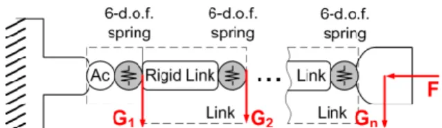
Elastostatic model of a serial robot is usually defined by its Cartesian stiffness ma-trix, which should be computed in the neighborhood of loaded configuration. Let us propose numerical technique for computing static equilibrium configuration for a general type of serial manipulator. Such manipulator may be approximated as a set of rigid links and virtual joints, which take into account elastostatic properties (Fig. 1). Since the link weight of serial robots is not negligible, it is reasonable to decompose it into two parts (based on the link mass centre) and apply them to the both ends of the link. All this loadings will be aggregated in a vector G 





loading applied to the i-th node-point. Besides, it is assumed that the external loading

F (caused by the interaction of the tool and the workpiece) is applied to the robot end-effector.

Following the principle of virtual work, the work of external forces G F, is equal to the work of internal forces τ caused by displacement of the virtual springs δθ







where the virtual displacements δtj can be computed from the linearized geometrical

model derived from ( ) θ

δ jδ , 1..

j  j n

t J θ , which includes the Jacobian matrices





J g q θ θ with respect to the virtual joint coordinates. So, expression (2) can be rewritten as



 





which has to be satisfied for any variation of δθ. It means that the terms regrouping the variables δθ have the coefficients equal to zero. Hence the force balance equa-tions can be written as

( ) T ( ) T θ θ θ 1 n j n j j 



These equations can be re-written in block-matrix form as

(G ) T (F ) T θ  θ   θ  τ J G J F (5) where (F ) ( ) θ θ n  J J , (G ) (1) ( ) θ θ θ T T T ... n      J J J , T T T 1 ... n     

G G G . Finally, taking into ac-count the virtual spring reaction τ_θ K_θθ, where





1 n

θ diag θ, ..., θ

K K K , the

desired static equilibrium equations can be presented as

(G ) T (F) T

θ   θ   θ

J G J F K θ (6)

To obtain a relation between the external loading F and internal coordinates of the kinematic chain θ corresponding to the static equilibrium, equations (6) should be solved either for different given values of F or for different given values of t. Let us solve the static equilibrium equations with respect to the manipulator configuration θ

and the external loading F for given end-effector position tg θ

 

 

 

 

(G ) T (F) T

θ  θ  θ ;  ; 

K θ J G J F t g θ G G θ (7) where the unknown variables are





Since usually this system has no analytical solution, iterative numerical technique can be applied. So, the kinematic equations may be linearized in the neighborhood of the current configuration θi

 

  



θ

1 1 ;

i  i  i  i  i

t g θ J θ θ θ (8)

where the subscript 'i' indicates the iteration number and the changes in Jacobians

(G ) (F )

θ , θ

J J and the auxiliary loadings G are assumed to be negligible from iteration to iteration. Correspondingly, the static equilibrium equations in the neighborhood of θi

may be rewritten as

(G ) T (F) T

θ   θ  i1 θ i1

J G J F K θ (9)

Thus, combining (8), (9) and expression for 1 (G ) T (F) T

θ ( θ θ )



   

θ K J G J F , the un-known variables F and θ can be computed using following iterative scheme







 







The proposed algorithm allows us to compute the static equilibrium configuration for the serial robot under external loadings applied to any point of the manipulator and the loading from the technological process.

3.2 Stiffness matrix

In order to obtain the Cartesian stiffness matrix, let us linearize the force-deflection relation in the neighborhood of the equilibrium. Following this approach, two

equili-briums that correspond to the manipulator state variables ( ,F θ t, ) and (Fδ ,F θδ ,θ tδ )t should be considered simultaneously. Here, notations δF, δt define small increments of the external loading and relevant displacement of the end-point. Finally, the static equilibrium equations may be written as

 

























where t, F G K, , _θ,θ are assumed to be known.

After linearization of the function g θ( ) in the neighborhood of the loaded equili-brium, the system (11), (12) is reduced to equations

(F ) θ (G ) (G ) (F ) (F ) θ θ θ θ θ δ δ δ δ δ δ δ       t J θ K θ J G J G J F J F (13)

which defines the desired linear relations between δt and δF. In this system, small variations of Jacobians may be expressed via the second order derivatives

(F) (F) θ θθ δJ H δθ, (G ) (G ) θ θθ δJ H δθ, where (G ) 2 (F) 2 θθ ₁ θθ 2 2 ; T T j n j j 

_

Also, the auxiliary loading G may be computed via the first order derivatives as δG  G  θ δθ

Further, let us introduce additional notation

(F ) (G ) (G ) T

θθ  θθ  θθ  θ   

H H H J G θ (15)

which allows us to present system (13) in the form

(F) θ (F) T θ θ θθ δ δ δ    _{ }      _{ }     _{ }   0 J t F 0 J K H θ (16)

So, the desired Cartesian stiffness matrices KC can be computed as





Below, this expression will be used for computing of the elastostatic deflections of the robotic manipulator.

3.3 Reduced mass matrix

To evaluate the dynamic behavior of the robot under the loading, in addition to the Cartesian stiffness matrix KC it is required to define the Cartesian mass matrix MC.

This mass matrix has the same dimension as KC and can be obtained using some

model reduction techniques. Comprehensive analysis and definition of this matrix have been proposed in [10]. Here, let us summarize the main results that will be used further.

To reduce the mass matrix dimension, model reduction techniques are applied for decreasing the size of the link mass matrices and also for the robot total mass matrix. Two main ways can be followed to reduce the size of the link mass matrices. The first one consists in discretizing the beam j into pj rigid links and springs and to express their displacements as a function of the beam extremity displacements. However, such numerical method must be repeated for each link and, thus, increases the size of the algorithm and decreases its efficiency. As a result, it is preferred to use the following procedure which allows analytical expressions to be obtained for the reduced link mass matrices.

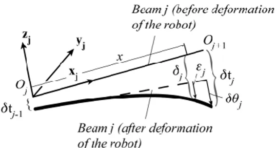
Let us consider the link j, modeled as a beam (Fig. 2). At this beam is attached a local frame represented by the vectors xj, yj and zj. Before any deformation of the

system, the beam j is linked to beams (j–1) and (j+1) at points Oj and Oj+1, respective-ly (Fig. 2). After deformation of the robot, the beam extremity located at Oj is

dis-placed from 1 2 6

1  1, 1, , 1

       

T j tj tj tj

δt and the one located at Oj+1 is displaced

from 1 2 6 , , ,          T j tj tj tj

δt , where the three first components of each vector cor-respond to the translational displacements along local xj, yj and zj axes, respectively,

and the three last components to the rotational displacements along the same axes. The general formula for the kinetic energy of an elastic Bernoulli beam is equal to:





_

In this expression, δ_j represents the velocity of the beam cross-section located at position x from the local reference frame (Fig. 2), Lj is the length of the beam j, j the mass density at cross-section x, Aj its area,

p j

I its torsional constant and y j

I , z j

I , the quadratic momentums along yj and zj, respectively.

For the l-th natural mode _l , the kinetic energy can be rewritten as:





_

j being the amplitude of the displacement of the beam cross-section located at posi-tion x from the local reference frame (Fig. 2).

In the Rayleigh-Ritz approximation, considering that the deformations due to the natural vibrations are similar to those obtained when an external load is applied at the robot end-effector only, each link of the structure will deform due to the stresses transmitted through the robot joints at points Oj. As a result, the deformations j of the beam cross-section can be approximated by the deformations of a tip-loaded beam





diag , , , , , 

j fj gj gj fj hj hj j

ε δθ (20)

where δθ_j ε_j





 

 





 





, 0.5 3 , 2 0.5

    

j j j j j j j j

f x x L g x x L x L h x x L x L (21)

As a result, the global displacement j of the beam cross-section at x can be ex-pressed as a sum of two terms:

  3 1 3 3             j j j I D δ δt ε 0 I , with _{ } 0 0 0 0 0 0 0 D x x      _  _     (22)

In this sum, the left terms corresponds to the displacement of the undeformed beam due to the displacement of the node located at Oj.

Introducing (20) to (22) into (9) leads to the following equation:





where the expressions of each components of matrix red j

M are given in [10]. Using these results, the total kinetic energy of the system for the l-th node is:







with diag





tot n

M M M and   ₀, ₁,, ₁, 

T T T T T n n

δt δt δt δt δt

Then, assuming that the first natural modes of vibrations, i.e. the modes that have the most energy, lead to deformations that are close to the static deformations of the robot under a load applied on the end-effector, the mass matrix can be recomputed into the Cartesian coordinates associated with the tool end-point using the Jacobian

matrix J_θ defined at expression (3) (which depend on the robot configuration q and computed with respect to virtual joint coordinates θ ) using following expression

θ

C θ θ

T



M J M J (25)

Thus, using expressions (25), it is possible to compute the reduced mass matrix

C

M for a given robot configuration q. The performances of this model reduction are shown in [10].

4

Machining process

Let us obtain the model of the cutting force which depends on the relative position of the tool with respect to the workpiece at each instant of machining. As follows from previous works [12], for the known chip thickness h, the cutting force Fc can be expresses as

 





where ap is a depth of cut, rk k0 1 depends on the parameters k∞, k0 that define the so called stiffness of the cutting process for large and small chip thickness h re-spectively (Fig. 3) and hs is a specific chip thickness, which depends on the current state of the tool cutting edge. The parameters k0, hs, r are evaluated experimentally for a given combination of tool/working material. To take into account the possible loss of contact between the tool and the workpiece, the above expression should be sup-plement by the case of h0 as

 

c

F h  h (27)

For the multi-edge tool the machining surface is formed by means of several edges simultaneously. The number of working edges varies during machining and depends on the width of cut. For this reason, the total force Fc of such interaction is a superpo-sition of forces Fc,i generated by each tool edge i, which are currently in the contact with the workpiece. Besides, the contact force Fc,i can be decomposed by its radial Fr,i and tangential Ft,i components (Fig. 4). In accordance with Merchant’s model [13], the t-component of cutting force Ft,i can be computed with the equation (26). The r-component Fr,i is related with Ft,i by following expression [14]

, ,

r i r t i

F k F (28)

where the ratio factor kr depends on the given tool/workpiece characteristics.

It should be mentioned that in robotic machining it is more suitable to operate with forces expressed in the robot tool frame {x,y,z}. Then, the corresponding components Fx, Fy (Fig. 4) of the cutting force Fc can be expressed as follows

Fig. 3. Fractional cutting force model Fc(h) Fig. 4. Forces of tool/workpiece interaction

Fig. 5. Meshing of the workpiece area

Fig. 6. Evaluating the tool/workpiece

inter-section Ai and computing the corresponding chip thickness hi , , 1 1 , , 1 1 co s sin sin co s z z z z n n x r i i t i i i i n n y r i i t i i i i F F F F F F             









where nz is the number of currently working cutting edges, φi is the angular position of the i-th cutting edge (the cutting force in z direction Fz is negligible here). So, the vector of external loading of the robot due to the machining process can be composed in the frame {x,y,z} using the defined components Fx, Fy as F=[Fx,Fy,0,0,0,0]T.

It should be stressed that the cutting force components Fr,i, Ft,i mentioned in equa-tion (26), (28) are computed for the given chip thickness hi, which should be also

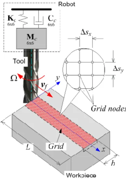
evaluated. Let us define model for hi using mechanical approach. Then the chip thick-ness hi removed by i-th tooth depends on the angular position φi of this tooth and it can be evaluated using to the geometrical distance between the position of the given tooth i and the current machining profile (Fig. 4). It should be mentioned, that the main issue here is to follow the current relative position between the i-th tooth and the working material or to define whether the i-th tooth is involved in cutting for given instant of process. Because of the robot dynamic behavior and the regenerative me-chanism of surface formation [15] this problem cannot be solved directly using kine-matic relations. In this case it is reasonable to introduce a special rectangular grid, which decomposes the workpiece area into segments and allows tracking the tool/workpiece interaction and the formation of the machining profile (Fig. 5).

Here, Steps Δsx, Δsy between grid nodes are constant and depend on the tool geo-metry, cutting condition and time discretization Δτ. Each node j ( j1,N_w , Nw is the number of nodes) of the grid can be marked as “1” or “0”: “1” corresponds to nodes situated in the workpiece area with material (rose nodes in Fig. 6), “0” corresponds to nodes situated in workpiece area that was cut away (white nodes in Fig. 6).

In order to define the number of currently cut nodes by the i-th tooth, the previous instant of machining process should be considered. Let us define Ai as an amount of working material that is currently cut away by the i-th tooth (Fig. 6). So, if node j marked as “1” is located inside the marked sector (green nodes in Fig. 6), it changes to “0” and Ai is increasing by  sx sy. Analyzing all potential nodes and computing

Ai, the chip thickness hi, removed at given instant of the process by the i-th tooth, can be estimated by hi  Ai Ri, i1,Nz. The angle Δφi determines the current

angu-lar position of the i-th tooth regarding to its position at the instant τ-Δτ and referred to the position of TCP at τ-Δτ.

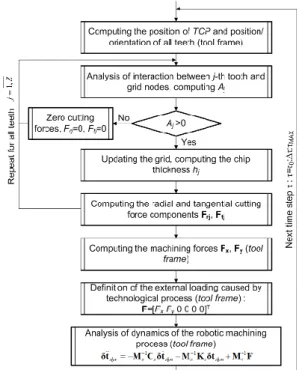
Described mechanism of chip formation and the machining force model (26) allow computing the dynamic behavior of the robotic machining process where models of robot inertia and stiffness are discussed in the section 3 of the paper. The detailed algorithm that is used in numerical analysis is presented in Fig. 7, where the analysis of the robot dynamics is performed in the tool frame with respect to the dynamic dis-placement of the tool δtdyn fixed on the robot end-effector around its position on the trajectory.

5

Compliance error compensation technique

In industrial robotic controllers, the manipulator motions are usually generated us-ing the inverse kinematic model that allows us to compute the input signals for actua-tors ρ0 corresponding to the desired end-effector location t0, which is assigned

as-suming that the compliance errors are negligible. However, if the external loading F

is essential, the kinematic control becomes non-applicable because of changes in the end-effector location. It can be computed from the non-linear compliance model as





where the subscripts 'F' and '0' refer to the loaded and unloaded modes respectively, and '|' separates arguments and parameters of the function f

 

To compensate this undeterred end-effector displacement from t0 to tF, the target

point should be modified in such a way that, under the loading F , the end-platform is located in the desired point t0. This requirement can be expressed using the stiffness

model in the following way





t denotes the modified target location. Hence, the problem is reduced to the solution of the nonlinear equation (31) for (F )

0

t , while F and t0 are assumed to be

given. It is worth mentioning that this equation completely differs from the equation

0

( | )

f



F t t , where the unknown variable is t. It means that here the compliance model does not allow us to compute the modified target point (F )

0

t straightforwardly, while the linear compensation technique directly operates with Cartesian compliance matrix [16].

To solve equation (31) for (F ) 0

t , similar numerical technique can be applied. It yields the following iterative scheme





Fig. 8. Procedure for compensation of compliance errors

Fig. 9. Implementation of compliance error compensation technique

where the prime corresponds to the next iteration, (0,1) is the scalar parameter ensuring the convergence. More detailed presentation of the developed iterative rou-tines is given in Fig. 8.

Hence, using the proposed computational techniques, it is possible to compensate a main part compliance errors by proper adjusting the reference trajectory that is used as an input for robotic controller. In this case, the control is based on the inverse kine-tostatic model (instead of kinematic one) that takes into account both the manipulator

geometry and elastic properties of its links and joints. Implementation of developed compliance error compensation technique presented in Fig. 9.

6

Experimental verification

The developed compliance error compensation technique has been verified expe-rimentally for robotic milling with the KUKA KR270 robot along a simple trajectory in aluminum workpiece. It is assumed that at the beginning of the technological process the robot is in the configuration q (see Table 1, Fig. 10). The parameters of the stiffness model for the considered robot have been identified in [17] and are pre-sented in Table 1. Link masses required for the mass matrix of the robot are prepre-sented also in Table 1.

For the milling, the cutter with the external diameter D=20 mm and four teeth (Nz=4) distributed uniformly over the tool is used. For the given combination of the tool and the workpiece material the following parameters correspond to the cutting force model defined in (26): k0=5106 N/m, hs=1.8 105



 _{m, r=0.1, k}r=0.3.

Fig. 10. Starting pose of the KUKA KR270

robot to perform the operation of milling

Fig. 11. Starting relative position of the tool

with respect to the workpiece

Table 1. Initial data for robotic-based milling

Joint coordinates, [deg]

q1 q2 q3 q4 q5 q6

90 -50 120 180 25 180

Joint compliances, [rad/N m]*10-6

k1 k2 k3 k4 k5 k6

0.26 0.15 0.26 1.79 1.52 2.13

Link masses, [kg]

m1 m2 m3 m4 m5 m6

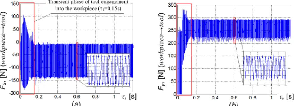
Fig. 12. Variation of machining force components Fx (a) and Fy (b) for whole milling process

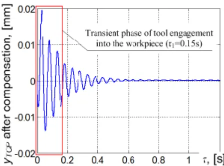
Fig. 13. Evolution of the tool dynamic

dis-placement δtdyn that is composed from xTCP and yTCP components

Fig. 14. Modified trajectory fy and correspond-ing feed rate vfy in y-direction, computed based

on the original dynamic displacement of the tool δtdyn

Taking into account that the workpiece has a straight borders let us assume that at the instant t=0 one of the teeth of the tool is in contact with the workpiece material as it is shown in the Fig. 11. It is also assumed that the machining process is performing with the constant feed rate vf=4 m/min (applied in x-direction of the robot tool frame) and the constant spindle rotation Ω=8000 rpm along the straight line of 80 mm. Expe-rimental verification and numerical simulation of the described case of the milling process with KUKA KR-270 robot using the algorithm shown in Fig. 7 allows us to trace the evolution of machining force x,y-components for the whole process (Fig. 12). The corresponding dynamic displacement of the tool around its current position on the trajectory is shown in Fig. 13.

In accordance with the obtained results the system robot/machining process realize complex vibratory motion. The high frequency component of this motion (about 700 Hz, Fig. 12) is related to the spindle rotation and the number of tool teeth Nz. In

cer-tain cases such behavior can excites the dynamics of the robot (natural modes) but this study remains out the frame of the presented paper. On the contrary, the low fre-quency component of robot/tool motion (about 7 Hz, Fig. 13), especially in the y-direction (that is perpendicular to the applied feed) influences directly the quality of final product. Such motion is related to the robot compliance and it can be compen-sated using the error compensation technique described in the paper. Hence, let us form the modified trajectory based on the dynamic displacement of the robot end-effector in the y-direction (Fig. 14).

It should be stressed that the time step between referenced points of this modified trajectory is limited with the characteristics of the controller used in the robot (in the presented case this step is chosen 0.05 sec). The corresponding feed rate vfy for the modified trajectory has been computed. So, this new data (feed fy and feed rate vfy) with the data defined in the beginning of this section allow us to compensate the tra-jectory error during machining caused by the robot compliance. The resulted compen-sated trajectory in the y-direction (in time domain) is presented in Fig. 15.

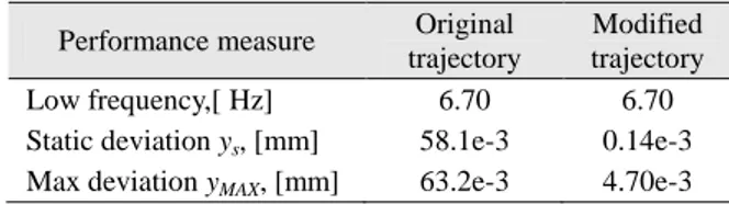
It should be noted that the part of the trajectory while machining tool is engaging into the workpiece does not have effect on the quality of final product (surface). Dur-ing this stage the contact area between the tool and the workpiece is increasDur-ing gressively. Hence, at each instant of processing the cutter corrects the machining pro-file and eliminates trajectory errors produced during all previous instants. On the con-trary, during the stage of machining with the fully engaged tool the trajectory in x,y-directions define directly the final machining profile and this part of trajectory is ana-lyzed here (Fig. 15). Comparison results presented in Fig. 13 and Fig. 15 are summa-rized in Table 2. So after applying error compensation technique the static deviation in y direction has been reduced from 0.058 mm to 0.00014 mm (99.8%). Maximum defilation in the machining profile has been reduced from 0.063 mm to 0.0047 mm (92.6%). Low frequency remained the same for both cases.

Hence, obtained results show that the developed compliance error compensation allows us significantly increase the accuracy of the robotic-based machining.

Fig. 15. Evolution of the dynamic displacement obtained after involving the error

Table 2. Milling trajectory accuracy before and after compliance error compensation

Performance measure Original trajectory

Modified trajectory

Low frequency,[ Hz] 6.70 6.70

Static deviation ys, [mm] 58.1e-3 0.14e-3 Max deviation yMAX, [mm] 63.2e-3 4.70e-3

7

Conclusion

In robotic-based machining, an interaction between the workpiece and technologi-cal tool causes essential deflections that significantly decrease the manufacturing accuracy. Relevant compliance errors highly depend on the manipulator configuration and essentially differ throughout the workspace. Their influence is especially impor-tant for heavy serial robots. To overcome this difficulty this paper presents a new technique for compensation of the compliance errors caused by technological process. In contrast to previous works, this technique is based on the non-linear stiffness mod-el and the reduced mod-elasto-dynamic modmod-el of the robotic based milling process.

The advantages and practical significance of the proposed approach are illustrated by milling with of KUKA KR270. It is shown that after error compensation technique significantly increase the accuracy of milling. In future the proposed technique will be integrated in a software toolbox.

8

Acknowledgements

The authors would like to acknowledge the financial support of the ANR, France (Project ANR-2010-SEGI-003-02-COROUSSO) and the Region “Pays de la Loire”, France.

9

References

1. Dépincé P., Hascoët J-Y., 2006. Active integration of tool deflection effects in end milling. Part 2. Compensation of tool deflection, International Journal of Machine Tools and

Man-ufacture, vol. 46, pp. 945-956

2. Altintas Y., 2000. Manufacturing automation, metal cutting mechanics, machine tool vi-brations and CNC design. Cambridge University Press, New York.

3. Eastwood S.J., Webb P., 2010. A gravitational deflection compensation strategy for HPKMs, Robotics and Computer-Integrated Manufacturing, vol. 26 pp. 694–702

4. Alici G., Shirinzadeh B., 2005. Enhanced stiffness modeling, identification and characteri-zation for robot manipulators. Proceedings of IEEE Transactions on Robotics, vol. 21, pp. 554–564.

5. Chen S., Kao I., 2000. Conservative Congruence Transformation for Joint and Cartesian Stiffness Matrices of Robotic Hands and Fingers. The International Journal of Robotics

6. Kövecses J., AngelesJ., 2007. The stiffness matrix in elastically articulated rigid-body sys-tems. Multibody System Dynamics. vol. 18(2), pp. 169–184.

7. Pashkevich A., Klimchik A., Chablat D., 2011. Enhanced stiffness modeling of manipula-tors with passive joints. Mech. and Machine Theory, vol. 46(5), pp. 662-679.

8. Tyapin I., Hovland G., 2009. Kinematic and elastostatic design optimization of the 3-DOF Gantry-Tau parallel kinamatic manipulator. Modelling, Identification and Control, vol. 30(2), pp. 39-56

9. Su H.-J., McCarthy J.M., 2006. A Polynomial Homotopy Formulation of the Inverse Static Analyses of Planar Compliant Mechanisms. Journal of Mechanical Design, vol. 128(4), pp. 776-786.

10. Briot S., Pashkevich A., Chablat D. Reduced elastodynamic modelling of parallel robots for the computation of their natural frequencies. 13th World Congress in Mechanism and Machine Science, 19 - 25 Juin, 2011, Guanajuato, Mexico.

11. Ritou M., Garnier S., Furet B., Hascoet J.Y., 2006. A new versatile in-process monitoring system for milling, Int. J. of Machine Tools & Manufacture, 46/15:2026-2035.

12. Brissaud D., Gouskov A., Paris H., Tichkiewitch S., 2008. The Fractional Model for the Determination of the Cutting Forces. Asian Int. J. of Science and Technology - Production

and Manufacturing, vol. 1, pp.17-25.

13. Merchant M.E., 1945. Mechanics of metal cutting process. I-Orthogonal cutting and type 2 chip. Journal of Applied Physics, vol.16(5), pp.267–275.

14. Laporte S., Knevez J.-Y., Cahuc O., Darnis P., 2009. Phenomenological model for drilling operation. Int. J. of Advanced Manufacturing Technology, vol.40, pp.1-11.

15. Tlusty J., Ismail F., 1981, Basic non-linearity in machining chatter. Annals of CIRP, Vol.30/1, pp.299-304.

16. Gong, C., Yuan J., Ni, J., 2000. Nongeometric error identification and compensation for robotic system by inverse calibration. International Journal of Machine Tools &

Manufac-ture, vol. 40(14) pp. 2119–2137.

17. Dumas C., Caro S., Garnier S., Furet B., 2011. Joint stiffness identification of six-revolute industrial serial robots, Robotics and Computer-Integrated Manufacturing, vol. 27(4), pp. 881-888.