UMR LEDa
Place du Maréchal de Lattre de Tassigny 75775 • Paris •Tél. (33) 01 44 05 45 42 • Fax (33) 01 44 05 45 45
D
OCUMENT DE
T
RAVAIL
DT/2019-01
DT/2016/11
Mothers and Fathers : Education,
Co-residence and Child Health
Loss: the Household Business Channel
Health Shocks and Permanent Income
Elodie DJEMAI
Yohan RENARD
Anne-Laure SAMSON
Mothers and Fathers : Education, Co-residence and Child Health
∗Elodie DJEMAI†, Yohan RENARD‡, and Anne-Laure SAMSON§
This version : January 15, 2019
R´esum´e
We use four waves of Demographic and Health Surveys from Zimbabwe to evaluate the effect of mother’s and father’s education on child health outcomes. We identify causal effects using the 1980 education reform. A simultaneous-equation model is estimated to take into account possible selection and endogeneity biases. Our results suggest some specialization within parents, as mothers and fathers do not affect the same health outcomes of their under-5 children. Fathers matter more than mothers, and mother’s education improves health only when she is matched to a low-educated man. There is selection in our sample, as is usual. The inverse Mills ratio capturing the likelihood of living with one’s father or mother significantly affects child health. Last, parental educational sorting is shown to be important, so that estimation that does not take both mother’s and father’s education into account will produce biased results.
JEL Codes : I10, I26, O12, J12, C36, C34
Keywords : Couples, Child’s Health, Education, Reform, Sub-Saharan Africa. R´esum´e
A partir de quatre vagues des Enquˆetes D´emographiques et de Sant´e conduites au Zimbabwe et de la r´eforme de l’´education men´ee en 1980, nous nous int´eressons `a l’effet causal respectif de l’´education de la m`ere et de l’´education du p`ere sur la sant´e des enfants de moins de 5 ans. Un mod`ele d’´equations simultan´ees est estim´e pour tenir compte d’´eventuels biais de s´election et d’endog´en´eit´e. Nos r´esultats sugg`erent une certaine sp´ecialisation au sein du couple parental puisque les m`eres et les p`eres n’influencent pas les mˆemes variables de sant´e de leurs enfants. Les p`eres semblent jouer un rˆole plus important que les m`eres, et l’´education des m`eres n’a d’effet sur la sant´e de leurs enfants que lorsque le niveau d’´education du p`ere est faible. Par ailleurs, nous mettons en ´evidence un ph´enom`ene de s´election dans notre ´echantillon. Les inverses des ratios de Mills, capturant la probabilit´e pour un enfant de vivre avec son p`ere ou avec sa m`ere, ont
∗Previous versions circulated under the title ”The impact of mother’s and father’s education on child’s health : Evidence from a quasi-experiment in Zimbabwe”. This project has benefited from the financial support of Health Chair - a joint initiative by PSL, Universit´e Paris-Dauphine, ENSAE, MGEN and ISTYA under the aegis of the Fondation du Risque (FDR). We would like to thank Eric Bonsang, Andrew Clark, Brigitte Dormont, Martin Karlsson, Carole Treibich, Jean-Noel Senne and participants at the LEGOS seminar (Paris, November 2017), the ”Journ´ees des Economistes de la Sant´e Francais” (Marseille, December 2017), the DIAL-Gretha Workshop (Paris, June 2018) and the 4th IRDES Workshop on applied health economics and policy evaluation (Paris, June 2018) who provided insightful comments. The usual disclaimer applies.
†Universit´e Paris-Dauphine, Universit´e PSL, IRD, LEDa, DIAL, 75016 Paris, France (corresponding author : elodie.djemai@dauphine.psl.eu. Universit´e Paris-Dauphine, Place du Marechal de Lattre de Tassigny, 75016 Paris (France)).
‡Universit´e Paris-Dauphine, Universit´e PSL, IRD, LEDa, DIAL, 75016 Paris, France. §LEM, Universit´e de Lille.
un effet significatif sur la sant´e des enfants. Enfin, nous montrons qu’´etant donn´e l’importance de l’homogamie d’´education, ne pas tenir compte simultan´ement de l’´education du p`ere et de la m`ere dans l’estimation conduit `a des r´esultats biais´es.
JEL Codes : I10, I26, O12, J12, C36, C34
Keywords : Couples, Sant´e des enfants, Education, R´eformes, Afrique Subsaharienne.
1
Introduction
The factors leading to better health are as important to economists as to other researchers in social sciences and policy-makers. Out of the eight Millennium Development Goals, three concern health and access to health care in developing countries. The lack of resources at both the govern-mental and individual levels has long been highlighted as the main barrier to improving health in developing countries. Poor people in low-income countries face a variety of health-related risks, with young children paying most of the global disease burden.
Of the 56.8 million deaths in 2016, 9.9% were of children under the age of five. In Africa this figure reached 31%.1
Over half of all deaths in low-income countries in 2016 were caused by so-called ”Group I” conditions, which include communicable diseases, maternal causes, conditions arising during pregnancy and childbirth, and nutritional deficiencies. By way of contrast, only 6.7% of deaths in high-income countries were due to these causes2
(World Health Organization 2018). These conditions caused 56% of all deaths in the WHO African Region in 2016. As such, most deaths could be avoided by adopting preventive actions (Banerjee and Duflo 2011) such as vaccination, water filtering, breastfeeding and the use of bed-nets. Education plays a key role here via its induced demand for prevention.
Since the model of health demand in Grossman (1972), the education-health relationship has appeared in a wide body of theoretical and empirical research. On average, the more-educated have better health and live longer than the less-educated (e.g. Lleras-Muney 2005). This is explained by lifestyles, working conditions and wages. Education not only affects the individual’s own health, but parental education also impacts the health of their children.
There are many channels through which education might affect health. The first is wealth. The 1. Authors’ calculations from World Health Organization (2018).
educated are likely to have better labor opportunities and higher wages, so that they can more likely afford the cost of prevention, treatment and private health-insurance, and have better access to health care and health centers. Second, the educated are more likely to understand the prevention messages they receive than their less-educated counterparts. Third, they have greater incentives to invest in preventive behaviors as, given the wage differential, the gap in terms of the future loss from illness is higher for the educated than for the less-educated. Last, education teaches discipline, compliance with rules and exams, exertion of effort and accepting constraints, as noted in Basu (2002). As such, it might help educated people to adopt costly preventive behaviors. Most of these mechanisms also apply when explaining why parental education might help improve child health.
Using the four waves of the Demographic and Health Surveys in Zimbabwe3
from 1999 to 2015, we examine the health outcomes of 21,976 children aged 0-4 born between 1994 and 2015. We compare the outcomes of children with educated mothers and fathers to those whose parents are less-educated.
The major problem in this comparison is the endogeneity of education, from the correlation between the unobservable characteristics leading to education and those leading to health invest-ments. Two examples of these unobserved characteristics are ability and time preference. Education and health are two indicators of human capital. As such, investing in education and investing in health both imply costly investment today for a future uncertain benefit. In addition, if educated parents are in better health than are less-educated parents, this affects the child’s health via the intergenerational transmission of health (Bhalotra and Rawlings 2011). We here exploit the exoge-nous increase in education produced by the 1980 reform to estimate the causal effect of mother’s and father’s education on child health.
A number of contributions have exploited exogenous variation in education to identify the causal relationship between education and outcomes such as employment, fertility and health. Recent articles have explored the relationship between education and health in developing countries, as 3. Zimbabwe is a low-income country of 16 million inhabitants (with GDP per capita of 2,085.7 current inter-national $ in PPP in 2017 (World Bank, World Development Indicators) located in Southern Africa. The under-5 mortality rate was 70.7 in 2015 (World Health Organization 2017). Life expectancy at birth was 61 in 1985, 44 in 2002 and 60.3 in 2015 (World Bank, World Development Indicators). The large fall at the end of the 1990s reflects high HIV prevalence. The HIV prevalence rate in the Demographic and Health Surveys was 21% for women aged 15-49 and 15.5% for men in 2005 (vs. 16.7 and 10.5 respectively in 2015).
major reforms to the latter’s school systems took place between 1970 and 2000. Using information on reforms allows us to estimate the causal effect of education on health outcomes in a quasi-experimental setting, as it provides exogenous variation in enrolment in Primary or Secondary school, the number of years of school or the likelihood of dropping out of school in instrumental-variable or regression-discontinuity approaches. Examples of these reforms are compulsory enrollment (Aguero and Bharadwaj 2014 ; Bharadwaj and Grepin 2015), the rise of the school-leaving age (Albouy and Lequien 2009 ; Kemptner et al. 2011), the supply of schools (Breierova and Duflo 2004 ; Silles 2009 ; Bhalotra and Clarke 2014), the implementation of Universal Primary Education policies (Behrman 2015 ; Osili and Long 2008) and changes in school fees (Silles 2009 ; Oyelere 2010). For instance, Grepin and Bharadwaj (2015) use the removal of Primary school fees and the building of Secondary schools in Zimbabwe to estimate the causal impact of mother’s secondary education on child mortality, as well as mothers’ age at marriage, age at first sex, age at first birth and ideal number of children.
Our work here also takes into account the marital education sorting of parents as an additional source of bias in the estimates, with the size of the bias being a priori even larger in articles that examine the effect of each parent’s education in separate models. If the correlation between education levels is high, the estimate of the effect of mother’s education on child’s health without controlling for father’s education may instead pick up the effect of father’s education. The bias may also come from unobservable characteristics (such as ability and time preference) that drive (un)educated people to match together. Marital sorting has been documented in developed and developing countries (eg. Azam and Djemai 2019 ; Chiappori et al. 2009 ; Van Bavel and Klesment 2017).
Last, co-residence between parents and children might also bias the estimates, as it might not be random in the population and covers a non negligible share of children : only 52% of our survey children aged 0-4 live with both parents. It is well-established in the literature that children growing up in single-parent households acquire less human capital, whether the parents divorced or one died (see Fitzsimons and Mesnard 2013 ; Adda et al. 2011). Living with both parents, compared to living with only one or neither, is not random and affects child health. We treat this as a selection issue,
as the education of the parent is not observed if he or she does not live in the same household as the observed child. The selection equations, one for each parent, are identified using exogenous variations in community practices (e.g. the % of mothers who give birth before being married). Our analysis of selection into co-residence provides new insights into the current literature on the education-health relationship that has to date neglected this dimension. Emran et al. (2018) documents this source of bias, calling it a truncation bias due to co-residency in the estimations of intergenerational mobility.
We also contribute to the literature on the respective role of mothers and fathers on child outcomes. The role of father’s education has been overlooked in the current literature, with only relatively few contributions (Case and Paxson 2001, Breierova and Duflo 2004, Apouey and Geoffard 2016, Chou et al. 2010, De Neve and Subramanian 2017, Lindeboom et al. 2009, Alderman and Headey 2017). This could reflect the common wisdom that mothers matter more than fathers in raising children. Another purely-empirical reason is that mothers are more likely than fathers to live with their children in many countries, leading to empirical challenges when trying to evaluate the role of fathers. Case and Paxson (2001) study the role of father’s and mother’s education and co-residence in child health in the US, but without modeling selection into co-residence or marital sorting.
The father’s contribution is modeled in three ways in recent work. First, the effect of the average mother’s and father’s education is estimated in Breierova and Duflo (2004). However, this does not allow us to consider differences between parents nor to use exposure to the reform as an instrumental variable, as men are usually older than their spouses. Second, two separate models are estimated, one controlling for mother’s education and the other for father’s education, as in Apouey and Geoffard (2016), Chou et al. (2010), De Neve and Subramanian (2017). From our viewpoint, this is debatable for two reasons : in the case of educational marital sorting, part of the effect of mother’s education may reflect that of the father’s, and there is no discussion about co-residence, even though the sample sizes vary from one estimation to the other. If one parent is absent because of divorce or death, the parent who is living with the child might compensate for the absence, and all the more so when (s)he is more educated and as such, has more room to
adjust. Some papers have explored the role of the absence of one parent on the formation of human capital and suggest that human capital is greatly affected. One example is Adda et al. (2011), who evaluate the long-term consequences of parental death and find that mothers and fathers have differential effects on child cognitive and non-cognitive skills. The third approach is to estimate the effect of both mother’s and father’s education in the same equation, as in Lindeboom et al. (2009) and Alderman and Headey (2017). In the latter, maternal and paternal education are referred to even for non-biological parents, whereas the effect might be different, given work on child fostering and step-mothers (e.g. Case and Paxson 2001). In this paper, we focus on the role of biological mothers and fathers, and estimate their respective effects along with the complementarities via an interaction between the two education levels in a single equation.
Grepin and Bharadwaj (2015) and De Neve and Subramanian (2017) are closest to our analysis, as they consider the 1980 education reform in Zimbabwe to estimate the causal effect of parental education on child health. Grepin and Bharadwaj (2015) focus on the effect of maternal education on child mortality, while we here estimate the effect of father’s and mother’s education on child’s current health and the conditions surrounding pregnancy and child birth. De Neve and Subramanian (2017) estimate the effect of both father’s and mother’s education on child malnutrition, as we do, but their estimation strategy differs from ours in several respects. First, they estimate the respective effects in separate regressions. Second, the outcomes are different. Third, they do not take marital sorting into account. Last, they do not model selection into co-residence.
The remainder of our paper is organized as follows. Section 2 describes the reform and its impact on parents’ education. Section 3 then presents the data and Section 4 the estimation strategy. The empirical results are described in Section 5, and the robustness checks and extensions appear in Section 6. Last, Section 7 concludes.
2
The policy intervention
Zimbabwe officially gained independence from the United Kingdom in 1980. Before indepen-dence, there were enormous inequalities in education between Whites and Blacks. For Whites, who represented only 3.5% of the population, education was free and compulsory until the age of 15
and admission to Secondary school was automatic after the pupils passed their Primary school final exam (Dorsey 1989). However, education was neither free nor compulsory for Blacks, who faced considerable selection at each grade. As a result, in the 1970s, only 4% of Black pupils were in Secondary school : the analogous figure was 43% for White pupils (Dorsey 1989). There was also inequality between boys and girls. In 1975, the girl/boy ratio was 85% in Primary education and 71% in Secondary education (see Table 1).
The first Black majority government - led by the Zimbabwe African National Union (ZANU) party - came to power with independence in 1980. Education was one of its top priorities for two reasons : (1) to satisfy the electorate, who considered education as the principal route to salaried employment and the modern way of life ; and (2) as it considered this to be the main instrument to expand and modernize the country (Dorsey 1989). The new Constitution therefore declared education as a fundamental human right (Education Act 2004). From 1980 on, the Government launched a vast intervention campaign to raise school attendance and the education of every child (Colclough et al. 1990 ; Aguero and Bharadwaj 2014 ; Grepin and Bharadwaj 2015). This expansion concerned both girls and boys and covered the whole country.
The main policy changes took place in 1980 and can be summarized as follows :
1. Primary education became free and compulsory for all pupils. Given the official duration of Primary education, all children would leave school with at least 7 years of education. 2. Admission to Secondary school became automatic for all pupils, whatever their performance
in the Primary-school final exam. Secondary education remained paying. 3. The removal of age-restrictions to allow older children to enter school.
4. The government changed the school zoning system that gave Whites access to the best schools ; it also introduced double-session schooling in almost all urban schools and some rural ones.
These reforms had a huge affect on child education, as shown in Figure 1, which comes from household-level data in the 1999, 2005, 2010 and 2015 Demographic and Health Surveys. Note that Primary education lasts 7 years and Secondary education 6 years,4
so pupils completing both 4. Lower Secondary education lasts 2 years while upper Secondary education lasts 4 years (WDI).
cycles have 13 years of education. The reform aimed to increase access to Secondary schools and so affected children at the end of Primary school, theoretically at age 14.5
We can thus define as being exposed to the Education reform all children who were 14 or younger in 1980, in other words children born after 1966. The vertical line in Figure 1 corresponds to the 1966 cohort : individuals born after 1966 are treated by the 1980 reform.
We have three potential measures of education in the DHS to evaluate the causal impact of edu-cation on health : years of eduedu-cation, attendance at Secondary school and Primary-school comple-tion. Grepin and Bharadwaj (2015) use Secondary-school attendance as their educational outcome. However, we do not believe that this is a valid variable. If treatment is defined by Secondary-school attendance, some ”untreated” individuals may have completed Primary school, whereas they would not have done so prior to the reform. They are therefore wrongly considered as untreated : the re-form did indeed increase their education. As a consequence, only Primary-school completion and years of education can be used as valid educational outcomes in this case. We prefer years of education, as this combines Primary-school completion and Secondary-school attendance.
Figure 1 depicts the proportion of mothers and fathers in each birth cohort who attended Secondary school for at least one year, who completed Primary school and their years of education. There are three main features. First, school attainment started to rise even among those not directly affected by the reform, in the sense that schooling was not compulsory for cohorts born before 1966. These cohorts were affected via easier school access after 1980. For example, women (men) born in 1950 had on average two (six) years of education, while the analogous figure for those born in 1960 was four (eight). Figures 1a and 1b show that this increase reflected both Primary- and Secondary-school attendance : the latter rose from effectively 0% (20%) for women (men) born in 1950 to 15% (40%) for those born in 1960. For the same two cohorts, Primary-school completion rose from 20% to 30% for women, and from 40% to 60% for men. The increase in education thus applied to both sexes.
Second, as shown in Figures 1a and 1b, the reform resulted in an expansion of pupils completing Primary school, but the largest change was found in Secondary education. It was this latter variable
that was used in Aguero and Bharadwaj (2014) and Grepin and Bharadwaj (2015) to estimate the causal effect of Secondary education. However, as noted above, we do not think that Secondary-school attendance is the best education-outcome variable to use for the instrumental estimation of the effect of education, as many of those who did not attend Secondary school were still affected by the education reform via the increase in Primary-school enrollment.
Last, even though the reform took place in 1980, the rise in school attendance was not immediate, taking four to five years as it took some time to train and recruit additional teachers and build new schools. The Government reconstructed all schools that had been destroyed during the war and built new Primary and Secondary schools, in particular in marginalized areas and disadvantaged urban centers (Kanyongo 2005). New teachers were also needed, and some of these were recruited from Secondary-school pupils. The World Development Indicators (World Bank) statistics in Table 1 show a huge jump in the number of Primary-school teachers between 1980 and 1985 and an even larger jump in Secondary-school teachers. As the number of enrolled pupils also rose, we can measure the potential quality of education by the number of pupils per teacher : this fell in Primary schools but rose in Secondary schools to reach a figure of 27 in 1990. Government expenditure on education rose sharply around the time of the reform, from 2.5% of GDP in 1980 to 12.5% in 1990.
Table 1 – Education indicators in Zimbabwe over the 1975-2000 period
1975 1980 1985 1990 1995 2000
Number of teachers - Primary 21,202 28,118 56,067 59,154 63,475 66,440 Number of teachers - Secondary 3,383 3,782 19,507 24,547 27,458 34,163 Teachers /1000 inhab. - Primary 3.44 3.86 6.33 5.65 5.45 5.31 Teachers /1000 inhab. - Secondary 0.55 0.53 2.25 2.41 2.42 2.79 Pupil/teacher ratio - Primary 40.69 43.92 39.50 35.78 39.11 37.03 Pupil/teacher ratio - Secondary 19.38 19.76 27.81 26.93 25.90 24.71
Girl/boy ratio - Primary 85.22 - 94.62 99.12 97.37 97
Girl/boy ratio - Secondary 71.26 - 68.46 88.00 83.66 88.00
Government funding (% of GDP) - 2.5 7.4 12.5 -
-Official entrance age - Primary 7 7 7 6 6 6
Official entrance age - Secondary 14 14 14 13 13 13
Figure1 – Mother’s and Father’s education by birth year 1966 0 .2 .4 .6 .8 Proport ions 1940 1960 1980 2000 Birth year Mothers Fathers
Attended secondary school
(a) Attended Secondary school
1966 0 .2 .4 .6 .8 1 Proport ions 1940 1960 1980 2000 Birth year Mothers Fathers
Completed primary school
(b) Completed Primary school
1966 0 2 4 6 8 10 Means 1940 1960 1980 2000 Birth year Mothers Fathers Years of education (c) Years of education
3
Data description
We use household-level data collected by the Demographic and Health Surveys in Zimbabwe. This survey is nationally representative of households and was collected in 1999, 2005, 2010 and 2015.6
The sampling is in two stages in each survey round. First, enumeration areas are selected based on the most recent available census. Second, a complete listing of the households living in the 6. We cannot use the earlier surveys as the 1994 survey does not allow us to link the household children to their fathers, and many of the child-health outcomes that we use in the analysis are not included.
selected enumeration areas (or communities) is established in order to randomly select the sampled households, and in the latter every women aged 15-49, whether permanent residents or visitors (who slept in the household the night before the survey) are eligible for interview. We here use the data files from the household roster and the female questionnaire. The male questionnaire is used to construct measures to predict the child’s probability of living with their father.
The household roster includes the complete list of household members and, for each member, age and the highest level of education. For children, the ID codes of the mother and father are listed if they live in the same household. As such, we have different types of households and family composition. We observe children who are not living with their parents (e.g. children fostered in another household) and children living with either one or both parents. By construction, if a sampled mother is not living with one of her children, this child is not a household member and is not present for the collection of anthropometric measures.
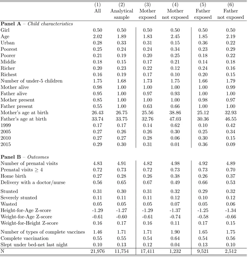
The analysis focuses on children aged between 0 and 59 months old, as mothers are asked specific questions about children in this age range as part of the female questionnaire. These questions cover delivery conditions, breastfeeding practices and vaccination. We also have anthropometric measures for children in this age group. The four rounds of survey data cover 21,976 children aged 0-4, of whom about half, 11,754, currently live with both parents and constitute our analytical sample.
The summary statistics for the entire sample and the analytical sample appear in Columns 1 and 2 of Table 2. A full description of the variables is provided in Appendix A. Over the entire sample, 50% of the children are girls, the average age is 2 and 28% live in urban areas. For 98% of the aged 0-4 children in sample households the mother is still alive, and for 95% the father is alive. Co-residence with the mother is 30 percentage points more likely than co-residence with the father : 85% of children live in the same household as their mother, and 55% in the same household as their father. The average age of mother at child birth is 26.4, and when the fathers are present their observed average age at birth is 33.7. This age difference corresponds to the usual age-difference figure found in existing work (e.g. d’Albis et al. 2012).
Table 2 – Descriptive statistics - Child characteristics and health outcomes
(1) (2) (3) (4) (5) (6)
All Analytical Mother Mother Father Father sample exposed not exposed exposed not exposed Panel A – Child characteristics
Girl 0.50 0.50 0.50 0.50 0.50 0.50 Age 2.02 1.89 1.83 2.45 1.85 2.19 Urban 0.28 0.33 0.31 0.15 0.36 0.22 Poorest 0.25 0.24 0.24 0.34 0.23 0.29 Poorer 0.21 0.19 0.20 0.25 0.18 0.22 Middle 0.18 0.15 0.17 0.21 0.14 0.18 Richer 0.20 0.23 0.22 0.12 0.24 0.16 Richest 0.16 0.19 0.17 0.10 0.20 0.15
Number of under-5 children 1.75 1.68 1.73 1.75 1.66 1.79
Mother alive 0.98 1.00 1.00 1.00 1.00 0.99
Father alive 0.95 1.00 0.97 0.93 1.00 1.00
Mother present 0.85 1.00 1.00 1.00 0.98 0.97
Father present 0.55 1.00 0.63 0.66 1.00 1.00
Mother’s age at birth 26.43 26.75 25.56 38.86 25.12 32.93
Father’s age at birth 33.74 33.75 32.76 47.03 30.36 46.55
1999 0.17 0.17 0.14 0.62 0.10 0.42
2005 0.27 0.26 0.26 0.30 0.25 0.34
2010 0.27 0.27 0.28 0.06 0.30 0.15
2015 0.29 0.30 0.31 0.01 0.36 0.09
Panel B – Outcomes
Number of prenatal visits 4.83 4.91 4.82 4.98 4.92 4.89
Prenatal visits ≥ 4 0.72 0.73 0.72 0.73 0.73 0.70
Home birth 0.27 0.28 0.26 0.38 0.26 0.37
Delivery with a doctor/nurse 0.56 0.65 0.67 0.49 0.66 0.53
Stunted 0.31 0.30 0.31 0.32 0.29 0.32 Severely stunted 0.11 0.11 0.11 0.12 0.10 0.12 Wasted 0.05 0.05 0.05 0.07 0.05 0.06 Height-for-Age Z-score -1.29 -1.27 -1.29 -1.37 -1.25 -1.34 Weight-for-Age Z-score -0.61 -0.60 -0.61 -0.74 -0.58 -0.66 Weight-for-Height Z-score 0.16 0.17 0.16 0.11 0.17 0.15
Number of types of complete vaccines 1.46 1.71 1.71 1.90 1.65 1.75
Complete vaccination 0.55 0.55 0.54 0.64 0.54 0.56
Slept under bed-net last night 0.10 0.13 0.12 0.04 0.13 0.10
N 21,976 11,754 17,411 1,232 9,521 2,512
Source :Authors’ calculations from the Demographic and Health Surveys (surveys 1999, 2005, 2010 and 2015).
Notes : Unweighted statistics. The analytical sample covers 0-4 children who currently live with both parents. Exposed mothers or fathers are those born in or after 1966.
The summary statistics for the outcome variables appear in Panel B. These can be grouped into three categories : (1) outcomes related to prenatal care and birth, namely the number of antenatal visits, having had at least four prenatal visits, having been born at home and having been assisted by medical staff at birth ; (2) malnutrition (nutrition Z-scores and malnutrition status) ; and (3) prevention (vaccination and sleeping under a mosquito bed-net).7
27% of sample children were born at home, and 56% of births were assisted by medical staff. The average number of antenatal visits is quite high, 4.8, compared to the recommendations of the WHO, and 72% of children had at least four antenatal visits. We use the anthropometric measures in the survey to construct common malnutrition indicators : 31% of young children are stunted, 11% severely stunted8
and 5% are wasted.9
The average number of types of complete vaccines is 1.46 and 55% of children received the complete recommended immunization package (BCG, Diphteria-Pertussis-Tetanus, measles) while 11% slept under a bed-net the night before the survey. Comparing the characteristics of sample children born to exposed mothers to those born to non-exposed mothers (columns 3 and 4, respectively), there is very little difference in some variables (child sex, for instance), while for others the observed differences reflect that, by definition, non-exposed mothers are older than non-exposed mothers and are more likely to come from the 1999 survey wave. Any differences thus contain both age and period effects. The observed children who are 0-59 months old at the time of the survey are more likely to be the first-borns of exposed mothers but not of non-exposed mothers, which is why age at birth is much higher in col. 4 than col. 3. Urban residence is much higher in the exposed sample than in the non-exposed sample, also due to large changes over time. Similar patterns are observed comparing children born to exposed (col. 5) and non-exposed (col. 6) fathers. Estimating a model with age and period effects is thus crucial to purge these observed differences between the treated and control groups.
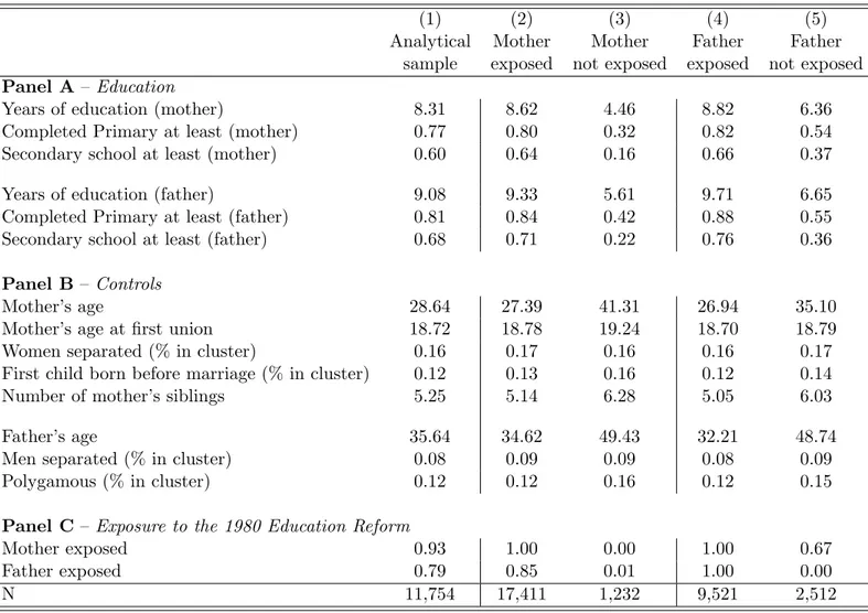
Mother and father education appear in Panel A of Table 3, and the full definition of the variables 7. The use of bed-nets is not asked in the 1999 survey wave. We do not analyze breastfeeding as 98% of children were breastfed.
8. Stunted children are too small for their age, that is their height-for-age Z-score is over two standard deviations below the reference value. Severely-stunted children have a HAZ score over three standard deviations below the reference value.
9. Wasted children are too thin for their height, that is their weight-for-height Z-score is over two standard deviations below the reference value.
is set out in Appendix Table A2. In the analytical sample in col. 1, the average number of years of schooling is 8.3 for mothers and 9.1 for fathers. 77% (81%) of mothers (fathers) completed Primary school, and 60% (68%) attended at least one year of Secondary school. Mothers’ average age is 28.6 and that for fathers 35.6. Mothers have, on average, five siblings. In our sample, 93% of the mothers were exposed to the reform, as were 79% of fathers (see Table 3, panel C). Mothers exposed to the reform have an average of 8.6 years of education, versus 4.5 years for those not exposed. 80% of the exposed mothers (32% of non-exposed mothers) completed Primary school, and 64% attended Secondary school (16% of the non exposed). On average, fathers exposed to the reform had 9.7 years of education versus 6.7 years for those not exposed. The impact of the reform is then about three to four additional years of education for both men and women. Men had much more education than women before the reform, and this gender difference remains after the reform. 88% of the fathers exposed to the reform completed Primary school versus 55% of those not exposed, and 76% attended Secondary school versus 36% of the non-exposed. Women have the same level of education as men for those born after the mid-1990s.
For the control variables defined at the enumeration-area level, the average proportion of women (men) who are separated, divorced or widowed in the community is 16% (8%), the proportion with first child born before marriage is 12%, and the average proportion of polygamous households is 12%.
4
Econometric specification
We estimate the joint impact of father’s and mother’s education on a number of child-health outcomes. Given the way in which Demographic and Health Surveys are collected (as described below), this is only possible when the child lives with both parents. Our econometric strategy therefore tackles three econometric issues : i) the endogeneity of father’s and mother’s education ; ii) marital education sorting (i.e. homogamy) ; and iii) selection into co-residence, as the sample of children who live with both parents is not random.
Table 3 – Descriptive statistics - Parents’ characteristics
(1) (2) (3) (4) (5)
Analytical Mother Mother Father Father sample exposed not exposed exposed not exposed Panel A– Education
Years of education (mother) 8.31 8.62 4.46 8.82 6.36
Completed Primary at least (mother) 0.77 0.80 0.32 0.82 0.54
Secondary school at least (mother) 0.60 0.64 0.16 0.66 0.37
Years of education (father) 9.08 9.33 5.61 9.71 6.65
Completed Primary at least (father) 0.81 0.84 0.42 0.88 0.55
Secondary school at least (father) 0.68 0.71 0.22 0.76 0.36
Panel B– Controls
Mother’s age 28.64 27.39 41.31 26.94 35.10
Mother’s age at first union 18.72 18.78 19.24 18.70 18.79
Women separated (% in cluster) 0.16 0.17 0.16 0.16 0.17
First child born before marriage (% in cluster) 0.12 0.13 0.16 0.12 0.14
Number of mother’s siblings 5.25 5.14 6.28 5.05 6.03
Father’s age 35.64 34.62 49.43 32.21 48.74
Men separated (% in cluster) 0.08 0.09 0.09 0.08 0.09
Polygamous (% in cluster) 0.12 0.12 0.16 0.12 0.15
Panel C– Exposure to the 1980 Education Reform
Mother exposed 0.93 1.00 0.00 1.00 0.67
Father exposed 0.79 0.85 0.01 1.00 0.00
N 11,754 17,411 1,232 9,521 2,512
Source :Authors’ calculations from the Demographic and Health Surveys (1999, 2005, 2010 and 2015 waves).
Notes :Unweighted statistics. The analytical sample refers to the sample of 0-4 children who are currently living with both parents. Exposed mothers (resp. fathers) are mothers (resp. fathers) who were born in or after 1966.
4.1 The endogeneity of education
In the child’s outcome equation, father’s and mother’s education are likely endogenous, leading to inconsistent estimates of the impact of education on health outcomes. Unobservable parental characteristics (such as time preference, ability and intrinsic motivation) make them more likely to invest both in their human capital (education) and the health of their children. In addition, education is correlated with parental health status, and healthy parents are more likely to have healthy children. Not controlling for parent’s own health status can then lead to a second source of endogeneity bias.
We address this endogeneity issue using instrumental variables, where the instrument is exposure to the reform : fathers and mothers born in or after 1966 (i.e. who were 14 or younger in 1980, or were not yet born) were exposed to the 1980 education reform.10
As shown in Figure 1, free and compulsory Primary education and easier access to Secondary education brought about an exogenous rise in years of education.
We estimate a 2SLS model with two first-stage regressions : one each for mother’s and father’s education. Those two-stage equations are defined as follows :
EducMiht= b M 0 + b M 1 T M + bM2 (B M −1966)1BM<1966+ b M 3 (B M −1966)2 1BM<1966+ bM4 (B M −1966)1BM≥1966+ bM5 (B M −1966)2 1BM≥1966+ Xiht′ b M 6 + Xht′ b M 7 + ǫ M iht (1) EducFiht= b F 0 + b F 1T F + bF2(B F −1966)1BF<1966+ b F 3(B F −1966)2 1BF<1966+ bF4(B F −1966)1BF≥1966+ bF5(B F −1966)21BF≥1966+ Xiht′ b F 6 + Xht′ b F 7 + ǫ F iht (2)
where i refers to the child (i = 1, ..., N ; N denotes the size of the analysis sample),11
h the 10. As a robustness check, we will remove from the analysis sample (i) children with at least one parent born between 1966 and 1970, as they may have benefited from higher school enrollment but of poor quality, and (ii) children who have at least one parent born between 1961 and 1965, as these parents are partially treated in that they were allowed to catch up.
11. We find the same results if we estimate these equations on the initial sample, i.e. the sample not restricted to having both mothers and fathers currently living with the observed child. These results are available upon request.
household and t the survey year. M denotes child i’s mother and F the father. The dependent variables (EducM
and EducF
) are the years of education reported by child i’s mother and father respectively. This measure of education is used in our baseline model ; Primary-school completion will appear an alternative in a sensitivity analysis. Note that our education variable is strictly positive for almost all parents in the sample : only 3% of fathers and 5% of mothers have no education. This small share of zero values justifies our use of OLS regressions in the first stage.
TM and TF are dummy variables for the post-reform period : TM (TF) is one if the mother
(father) was born in or after 1966, i.e. was 14 or younger in 1980, and zero otherwise. The direct impacts of the policy reform on education are given by bM
1 for the mother and b F
1 for the father. To
reflect the different trends in education before and after the reform, as in Figure 1, we include pre-and post-reform quadratic trends, denoted respectively by (B−1966)1B<1966and (B−1966)
2
1B<1966
pre-reform and (B − 1966)1B≥1966 and (B − 1966)21B≥1966 post-reform, where B is the parent’s
birth year. The number of siblings is added to the list of instruments for the mother, but is not available for fathers. Xiht and and Xht are sets of exogenous child and household variables that
are also included in the outcome equation. Given our econometric strategy, other variables need to be included in these first-stage regressions : these will be described in Section 4.4, where the final model is set out.
Table 4 – The First-Stage estimates for mothers and fathers (1) (2) (3) (4) EducationM EducationF EducationM EducationF Exposed 1.244∗∗∗ 0.460∗∗ 3.101∗∗∗ 2.292∗∗∗ (0.445) (0.207) (0.167) (0.103) Pre-reform trend 0.329∗∗ 0.243∗∗∗ (0.159) (0.026) Pre-reform trend2 0.014 0.003∗∗∗ (0.011) (0.001) Post-reform trend 0.121∗∗∗ 0.021 (0.019) (0.017) Post-reform trend2 -0.003∗∗∗ -0.002∗∗∗ (0.001) (0.001)
Number of mother’s siblings -0.004 -0.008
(0.011) (0.011) Constant 8.223∗∗∗ 12.139∗∗∗ 7.450∗∗∗ 10.715∗∗∗ (0.664) (0.833) (0.542) (0.837) N 10,851 11,653 10,851 11,653 Adjusted R2 0.39 0.41 0.38 0.38 F 59.17 73.56 62.67 70.29 p-value (F) 0.000 0.000 0.000 0.000 F (excluded instruments) 76.10 173.91 173.67 497.42
pvalue (excluded instruments) 0.000 0.000 0.000 0.000
Control variables X YES YES YES YES
Region FE YES YES YES YES
Year FE YES YES YES YES
Region × Year FE YES YES YES YES
Source :Authors’ calculations from the Demographic and Health Surveys.
Notes : ∗p <0.10, ∗∗ p <0.05, ∗∗∗ p <0.01. Robust standard errors clustered at the enumeration area level are in parentheses. Education is years of education. The control variables X are child sex and age, urban residence and household-wealth quintiles. The F-statistic of excluded instruments is obtained from the estimation of equations (1) and (2). There is no correction for selection into co-residence.
The estimation results from the first-stage equations (1) and (2) are presented in columns 1 and 2 of Table 4, respectively. Note that, for identification purpose, those equations also control for all the exogenous variables in the outcome equation.12
The average number of school years is 1.2 years 12. In practice, as the first-stage and outcome equations are estimated simultaneously, we have as many first-stage
higher for mothers exposed to the reform compared to the non-exposed, with a corresponding figure of 0.46 years for fathers. The reform therefore had a much greater effect on mothers than fathers (and significantly so at the 1% level).13
Our first-stage regressions are convincing ; the F-statistics on excluded instruments (exposure to the reform and its trends, along with the number of siblings for the mothers only) indicate that our instruments are not weak (F=121.7 for mothers ; F=141.6 for fathers).
Columns 3 and 4 relax the assumption of pre- and post-reform trends in access to education, and estimate years of education using only the binary treatment variable, as well as the number of siblings in the mothers’ equation. The coefficient on reform exposure is much larger here in col. 3 (col 4) than in col. 1 (col. 2), with a very large estimated reform effect of 3.1 more education years for mothers and 2.3 more years for fathers, with again the difference between the two point estimates being significant at the 1% level.
4.2 Selection into marriage
Marital educational sorting may be an issue in our model. In the analysis sample, 89% of mothers who completed Primary school married men who also completed Primary school, and 85% of mothers who attended Secondary school married men who also attended Secondary school. There is consequently substantial correlation between mother’s and father’s years of education : 0.63. Women and men with similar education tend to live with or marry each other. As a result, the unobservable characteristics that explain mothers’ education (such as intrinsic motivation) may well be correlated with unobservables that explain fathers’ education.
In our final model, mother’s and father’s education are therefore estimated simultaneously, taking into account the correlation between the residuals of both equations (ǫM
iht and ǫ F
iht). We find
a positive and very-significant correlation (0.415) between these residuals (see Appendix Tables regressions as outcomes. Given that the sample size varies slightly between outcomes, depending on the number of missing values, the results from the first-stage estimations may also vary. However, this turns out not to be the case : the results are very similar across outcomes and sample sizes. In this Section, and in the paper in general, we only report and comment on the first-stage regressions for the entire analytical sample. In the final specification, described in Section 4.4, the Inverse Mills ratio is included as a right-hand side variable to correct for possible selection bias.
13. The pre-reform level of education differs between mothers and fathers : see the descriptive statistics in Table 3 and Figure 1.
B2-B4) : men and women with similar intrinsic incentives or aspirations towards human-capital investment tend to live and have children with each other.
4.3 Selection into co-residence
Our ability to observe the dependent and independent variables of interest depends on the five types of setting in the data, as summarized in Table 5.
Table 5 – Selection issues
Presence in the sampled household Education Type of health data Child Mother Father Mother’s Father’s current Birth N in the hh in the hh in the hh education education status info
(1) (2) (3) (4) (5) (6) (7) (8)
Type 1 2,863 No Yes Yes 8.35 NA No Yes
Type 2 11,773 Yes Yes Yes 8.30 9.08 Yes Yes
Type 3 3,217 Yes No No NA NA Yes No
Type 4 286 Yes No Yes NA 9.17 Yes No
Type 5 7,249 Yes Yes No 8.4 NA Yes Yes
The analytical sample used to estimate the effect of mother’s and father’s education on child-health outcomes is restricted to sampled children who live with both parents (household composition of Type 2). If the three are listed as household members, we can match the children to their parents using their IDs, and the educational attainment of each parent is observed. In order to observe current health outcomes, we need either the mother to live in the household (as the birth history is asked of each mother) or the child to live in the household (and thus be present when the anthropometric measures are taken). Both types of outcomes are observed when the child and mother live in the same household.
In the four other cases, we do not have all of the necessary information (child-health outcomes and father’s and mother’s education). The different cases are summarized in Table 5. In Type 1 the child is not a household member, while the mother is (and maybe the father too). The mother declares the child in the birth history, but the child does not appear in the survey either because he/she is dead or is fostered in another household. As these children are not listed in the household roster, we cannot match them to their fathers, so that father’s education is unobserved. There are
2,863 children of this type who will not appear in our analysis, including in the selection equation. Children of Types 3, 4 and 5 currently live in the sampled households but are left out of the analysis sample as they do not live with both parents. Type-3 children live with neither parent, Type-4 children with their father but not their mother, and Type-5 children with their mother only. We have missing data on the birth-outcome variables for Types 3 and 4 children as the mother is not in the sampled household and so does not reply to the questionnaire recording that information. Current child weight and height is observed when the child is present in the household, that is for children of Types 2 to 5.
Of the 22,525 sampled children aged 0-4, 52.3% live with both parents (Type 2), 14.3% with neither (Type 3), 1.3% with their father only (Type 4) and 32.2% with their mother only (Type 5). The Type-2 percentage is fairly stable over time : 52% in 1999, 53% in 2005, 53% in 2010 and 55% in 2015. This low percentage of children living with both parents is not particular to Zimbabwe, although it does have one of the lowest percentages among African countries (according to Pilon and Vigniki (2006), who refer more broadly to children aged below 15).14
There are no great differences in school attainment across types. When mother’s education is observed, this varies from 8.3 to 8.4 years (see col. 5 of Table 5), and for fathers from 9.08 to 9.17 (col. 6). However, Table 2 shows that our analytical sample differs somewhat from the whole sample : households in the analytical sample are richer, and are more likely to live in urban areas and have younger children. From Panel B, we see that their children also have better health outcomes, although these gaps are not large. Except for having been born with the help of medical staff and the number of vaccines, the statistics in columns 1 and 2 are quite similar.
Our estimations may suffer from selection bias due to the coresidence restriction, for which we need to correct. The unit of analysis here is all children 0-4 living in sampled households (i.e. children of Types 2-5), and selection bias is addressed via Heckman’s two-step procedure.15
We 14. In Namibia, only 26% of children below the age of 15 live with both parents, with an analogous figure of 33% in South Africa. This percentage rises to about 50% in Zimbabwe and Rwanda. But most countries have higher figures, such as Benin (65%), Ethiopia (71%) and Burkina Faso (78%) (Pilon and Vigniki 2006).
15. We estimate a selection equation to explain why parents may not live with their children. Only 2% of mothers and 5% of fathers of sample children are dead. Fathers/mothers who do not live with their child are therefore mainly parents who have decided not to live together : divorcees, temporary migrants who quit the household and those who have entrusted their child to somebody else’s care. We hypothesise that all of these potential (unobserved) reasons can be summarized by one single selection equation, a hypothesis that is of course debatable.
estimate two probit selection equations, one each for the mother and father. Let CoresidenceM iht
(CoresidenceF
iht) be a dummy for child i living with her mother M (father F ) in survey t, and zero
otherwise. We have :
CoresidenceMiht = 1 if Coresidence∗Miht >0, 0 otherwise
CoresidenceFiht = 1 if Coresidence∗Fiht>0, 0 otherwise
where Coresidence∗M
iht and Coresidence∗Fiht are latent variables defined as follows :
Coresidence∗Miht = a M 0 + Ziht′Ma M 1 + Xiht′ a M 2 + Xht′ a M 3 + µ M iht (3) Coresidence∗Fiht = a F 0 + Ziht′Fa F 1 + Xiht′ a F 2 + Xht′ a F 3 + µ F iht (4)
As before, i indexes the child (i = 1, ..., NT, where NT denotes the size of the initial sample), h
the household and t the year of the survey.
The estimation of these selection equations requires exclusion restrictions, i.e. variables that influence co-residence but have no direct effect on the outcome. We use community-level variables. For the mother, we use two variables (ZM
iht) : the proportion of sampled women who gave birth to
their first child before getting married in each community, and the proportion of sampled women who are currently divorced, separated or widowed in each community. For fathers, the excluded variables ZF
iht are the proportion of sampled men currently divorced, separated or widowed in
each community and the percentage of sampled men living in a polygamous household in each community. There are 1,418 different communities in our analytical sample, each of which is large enough to be distinct from the individual considered (comprising, on average, 11 households and 65 individuals). The models also inlcude child (X′
iht) and household (Xht′ ) characteristics in the
Table 6 – Selection equations for mothers and fathers (Equations (3) and (4))
(1) (2)
Mother present Father present
Separated (% in cluster) -0.657∗∗∗ -0.741∗∗∗
(0.126) (0.116) First child born before marriage (% in cluster) -0.682∗∗∗
(0.145) Polygamous (% in cluster) 0.436∗∗∗ (0.116) Age -0.301∗∗∗ -0.069∗∗∗ (0.007) (0.006) Girl 0.003 -0.000 (0.021) (0.018) Urban 0.298∗∗∗ 0.209∗∗∗ (0.056) (0.053) Poorest 0.120∗ -0.108∗ (0.062) (0.058) Poorer -0.049 -0.241∗∗∗ (0.061) (0.057) Middle -0.107∗ -0.367∗∗∗ (0.059) (0.056) Richer 0.121∗∗∗ -0.057 (0.046) (0.039) Constant 2.263∗∗∗ 1.093∗∗∗ (0.167) (0.138) N 21,975 21,924 Pseudo R2 0.11 0.06 Correctly specified 63.78 62.02
Region FE YES YES
Year FE YES YES
Region × Year FE YES YES
Source :Authors’ calculations from the Demographic and Health Surveys.
Notes :∗ p <0.10,∗∗ p <0.05,∗∗∗p <0.01. Robust standard errors clustered at the enumeration area level are in parentheses.
The selection-equation estimation results (3) and (4) appear in Table 6, cols. 1 and 2 respectively. All of the instruments are significantly related to the probability of co-residence at the 1% level, and are of the expected sign. We find that the greater the proportion of sampled women who gave birth to their first child before getting married in each community and the higher the proportion of sampled women who are currently divorced, separated or widowed in each community, the lower the probability that the child live with their mother. Equally, the higher the proportion of men who are currently divorced, separated or widowed in the community, the lower is the probability that the child live with their father, and the higher the proportion of men living in polygamous households, the higher the probability that the child live with their father.16
4.4 Final specification
Our final specification aims to identify the effect of parental education on a number of child-health outcomes. We address education endogeneity via the policy reform that allowed some pa-rents to enroll in school and stay longer in school. We do so via 2SLS estimation. Selection into co-residence is taken into account using a two-step Heckman selection model, and marital homo-gamy using correlated error terms between fathers’ and mothers’ education. We use the procedure described in Wooldridge (2002, Chapter 17) to estimate a full model that takes all these issues into account in the five-equation model described below.
16. We may have expected this correlation to be of the opposite sign. However, polygamous fathers in Zimbabwe usually live in the same house with their different wives, especially in rural areas (OECD 2010).
Coresidence∗Miht = a M 0 + Ziht′Ma M 1 + Xiht′ a M 2 + Xht′ a M 3 + µ M iht; i = 1, ..., NT (5) Coresidence∗Fiht= a F 0 + Ziht′Fa F 1 + Xiht′ a F 2 + Xht′ a F 3 + µ F iht; i = 1, ..., NT (6) EducMiht= b M 0 + b M 1 T M + bM2 (B M −1966)1BM<1966+ b M 3 (B M −1966)21BM<1966 +bM4 (B M −1966)1BM≥1966+ b M 5 (B M −1966)21BM≥1966+ b M 6 λ M iht+ Ziht′Mb M 7 +bF 6λ F iht+ Ziht′Fb F 7 + Xiht′ b M 8 + Xht′ b M 9 + ǫ M iht; i = 1, ..., N (7) EducFiht= b F 0 + b F 1T F + bF2(B F −1966)1BF<1966+ b F 3(B F −1966)2 1BF<1966 +bF 4(B F −1966)1BF≥1966+ bF5(B F −1966)2 1BF≥1966+ bF6λ F iht+ Ziht′Fb F 7 +bM6 λ M iht+ Ziht′Mb M 7 + Xiht′ b F 8 + Xht′ b F 9 + ǫ F iht; i = 1, ..., N (8) Hiht = c0+ cM1 Educ M iht+ c F 1Educ F iht+ c F M 1 Educ F iht∗Educ M iht+ c M 2 λ M iht+ c F 2λ F iht +Ziht′Mc M 3 + Ziht′Fc F 3 + Xiht′ c4+ Xht′ c5+ νiht; i = 1, ..., N (9)
In equation (9), Hiht is child health, and EducMiht and Educ F
iht are continuous variables for
mo-ther’s and famo-ther’s years of education respectively. We also include an interaction between momo-ther’s and father’s education, EducF
iht∗Educ
M
iht, which allows us to test for complementarity between the
two.
N is the size of the analytical sample. The outcome equation includes a number of exogenous variables that also appear in the selection and first-stage equations : Xiht includes child
characte-ristics (age and sex) and Xht household characteristics (household wealth quintiles, urban location,
effects). We could not include religion or household ethnicity.17
The year dummies (1999, 2005, 2010 and 2015), region fixed-effects and their interactions are included in all equations.
As described in Wooldridge (2002), we correct for any selection bias by adding the Inverse Mills ratios from the probit estimation of equations (5) and (6) to both the first-stage ((7) and (8)) and outcome (9) equations. The two Inverse Mills ratios are λM
and λF
, and a test for selection bias is cM
2 = 0 and c F
2 = 0 in (9).
All exogenous variables should appear in the selection equation and be listed as instruments in the 2SLS procedure. However, in our case, some exogenous variables (such as the exposure to the reform variables) cannot be included in the selection equation as they are not observed for fathers and mothers who do not live with their child. Equations (5) and (6) are estimated separately via probits, and Equations (7) to (9) are estimated simultaneously using linear-probability models. This joint estimation allows us to take into account any correlation between the error terms : ǫM
iht and
ǫFiht may be correlated due to assortative matching ; ǫ M
iht and νiht as well as ǫ F
iht and νiht may also
be correlated if mothers (fathers) have intrinsic characteristics that influence both their choice of education and their ability to improve their child’s health. We later discuss the sign and significance of all these correlations. We do not consider any correlation between µM
iht and ǫ M iht, µ F iht and ǫ F iht or µMiht, µ F
iht and νiht, as these error terms refer to samples of different sizes. Last, note that standard
errors are clustered at the enumeration area level in all equations as proportions computed at the enumeration area level are included in the set of right-hand side variables.
5
Results
5.1 The impact of mother’s education only
We start our analysis by looking at the impact of mother’s education on child-health outcomes, as this has been the focus of the literature on parental education and child health. As such, the role of the father in terms of his living with his children and education is not taken into account.
17. There is insufficient variation in religion : depending on the survey waves, 90-95% of mothers are Christians and 5-10% Atheists, and 65-80% of fathers are Christians and 20-25% Atheists. Moreover, ethnicity is not available in our survey waves.
The most naive approach is to estimate the effect of mother’s education in the sample of children living with their mother, whatever the situation of the father : the child can either live with both parents or with the mother and not the father. We can argue that the estimated effect of mother’s education here is unreliable for a number of reasons. First, if the child lives with both parents, and the father and mother have similar education, not controlling for father’s education may overestimate the effect of mother’s education, as the latter captures part of that of the father. Second, if the father does not live with his child, the educated mother might compensate for the father’s absence so that the estimated effect might be larger than it would have been in the presence of the father.
We tackle these issues by estimating the effect of mother’s education in different samples : first the sample of children who live with their mother (with the father being present or not) ; second, the sample of children who live with their mother and not their father ; and third, the sample of children who live with both parents. We compare the results across the different samples using the 95-percent confidence intervals.
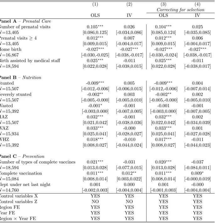
Table 7 shows the benchmark results for the sample of all mothers living with their child, whatever the situation of the father. We then estimate equations (5), (7) and (9) without including any information on the father. Four estimates are shown : the OLS estimate (column 1), the 2SLS estimate (column 2), the OLS estimate correcting for selection (column 3) and the 2SLS estimate correcting for selection (column 4). The results in column 4 come from our preferred specification that deals with all the estimation issues discussed above ; this corresponds to the estimation of equation (9). However, columns 1 to 3 help us to understand how our results change when correcting for the endogeneity of education and selection.
In the OLS specification in column 1, the education coefficient has the expected sign, as more education is associated with better health : in Panel A there are more prenatal visits, a greater probability of having attended at least four prenatal visits and the birth being assisted by a doctor or a nurse, and a lower probability of home birth. In Panel B, mother’s education is also associated with improved child nutrition, reducing the probability of child stunting, severe stunting and wasting, and increasing the three Z-scores (height-for-age, weight-for-age and weight-for-height). Last, the OLS
estimates in Panel C suggest that mother’s education increases vaccine use. All of the estimated coefficients are significant, except for that on bed-net use (although mother’s education may be associated with children living in lower-risk malaria environments). We here look at the use of bed-nets, rather than the fact of owning them, so that we estimate their effective coverage.
Column 2 reports the IV point estimates of mother’s education on the various outcomes. The IV estimates for many outcomes are of the same (positive) sign as the OLS estimates, but are not significant. The effect of mother’s education remains statistically significant on the probabilities of home birth and complete vaccination. The same results are found in column 4, taking into account selection into co-residency, except that there is a counterintuitive negative effect on the number of vaccines. More generally, the results suggest that selection into co-residency with the mother does not drive the previous results, as the findings are similar between cols. 1 and 3 for OLS, and between cols. 2 and 4 for IV.
The findings in cols. 1 and 2 of Table 7 can be compared to those in De Neve and Subdramanian (2017) for the probabilities of being stunted and wasted via OLS and IV. Our results are in line with theirs, as the OLS estimates of the effect of maternal schooling are negative and significant, while the IV estimates are insignificant.
We now restrict the sample to children who live with their mother and whose father is not present in the household (Table 8), reducing the sample from about 18,000 observations to about 7,000. In column 4 we find, as in Table 7, that children with more-educated mothers have a lower probability of being born at home. While mother’s education significantly influences the Z-scores and nutrition status in the OLS models (cols. 1 and 3), the IV coefficients are insignificant in cols. 2 and 4. The point estimates are however very similar to those in Table 7. On the contrary, the coefficients for the prevention variables are no longer significant in Table 8 (even though their values lie in the confidence intervals of those in Table 7). Prevention behaviors may then be more affected by fathers, so that the coefficients on these variables in Table 7 are not accurately estimated. The impact of mother’s education may partly capture that of father’s education (especially if they have similar education). This also means that when the father does not live with his children, the mother does not compensate for his absence by adopting preventive behaviors.
Table 7 – The impact of mother’s education only (whole sample)
(1) (2) (3) (4)
Correcting for selection
OLS IV OLS IV
Panel A– Prenatal Care
Number of prenatal visits 0.105∗∗∗ 0.026 0.104∗∗∗ 0.025
N=13,405 [0.086,0.125] [-0.034,0.086] [0.085,0.124] [-0.035,0.085]
Prenatal visits ≥ 4 0.012∗∗∗ 0.007 0.012∗∗∗ 0.006
N=13,405 [0.009,0.015] [-0.004,0.017] [0.009,0.015] [-0.004,0.017]
Home birth -0.027∗∗∗ -0.027∗∗∗ -0.027∗∗∗ -0.027∗∗∗
N=16,867 [-0.030,-0.025] [-0.038,-0.017] [-0.030,-0.024] [-0.038,-0.017]
Birth assisted by medical staff 0.025∗∗∗ -0.011 0.025∗∗∗ -0.011
N=18,594 [0.022,0.028] [-0.038,0.015] [0.022,0.028] [-0.038,0.017] Panel B– Nutrition Stunted -0.009∗∗∗ 0.005 -0.009∗∗∗ 0.004 N=15,507 [-0.012,-0.006] [-0.006,0.015] [-0.012,-0.006] [-0.007,0.014] Severely stunted -0.002∗∗ 0.003 -0.002∗∗ 0.002 N=15,507 [-0.005,-0.000] [-0.005,0.010] [-0.005,-0.000] [-0.005,0.010] Wasted -0.001∗ -0.001 -0.001 -0.001 N=15,392 [-0.003,0.000] [-0.007,0.005] [-0.003,0.000] [-0.007,0.005] HAZ 0.032∗∗∗ -0.001 0.032∗∗∗ 0.002 N=15,507 [0.021,0.042] [-0.038,0.036] [0.022,0.042] [-0.034,0.039] WAZ 0.033∗∗∗ -0.000 0.033∗∗∗ 0.001 N=15,934 [0.025,0.041] [-0.028,0.027] [0.025,0.041] [-0.027,0.028] WHZ 0.018∗∗∗ -0.010 0.017∗∗∗ -0.011 N=15,392 [0.008,0.027] [-0.044,0.024] [0.008,0.027] [-0.044,0.023] Panel C– Prevention
Number of types of complete vaccines 0.021∗∗∗ -0.031 0.020∗∗∗ -0.037
N=18,594 [0.013,0.028] [-0.077,0.015] [0.013,0.028] [-0.084,0.011]
Complete vaccination 0.011∗∗∗ 0.012∗∗ 0.011∗∗∗ 0.009∗
N=15,084 [0.008,0.014] [0.003,0.022] [0.008,0.014] [-0.000,0.019]
Slept under net last night 0.001 0.000 0.001 -0.000
N=14,760 [-0.002,0.003] [-0.004,0.004] [-0.001,0.003] [-0.004,0.004]
Control variables X YES YES YES YES
Control variables Z NO NO YES YES
Region FE YES YES YES YES
Year FE YES YES YES YES
Region × Year FE YES YES YES YES
Source :Authors’ calculations from the Demographic and Health Surveys. Notes :∗
p <0.10,∗∗
p <0.05,∗∗∗
p <0.01. 95% confidence intervals in brackets. Robust standard errors clustered at the enumeration area level. The control variables X are child sex and age, urban residence and household-wealth quintiles. Columns (3) and (4) also control for the Inverse Mills ratio obtained for mothers. The control variables Z are the proportions of sampled women who were previously married and who gave birth to their first child outside of marriage in the cluster.
Table 8 – The impact of mother’s education only (mothers who live without the father)
(1) (2) (3) (4)
Correcting for selection
OLS IV OLS IV
Panel A– Prenatal Care
Number of prenatal visits 0.081∗∗∗ 0.076 0.081∗∗∗ 0.077
N=5,093 [0.052,0.111] [-0.024,0.177] [0.051,0.111] [-0.023,0.176]
Prenatal visits ≥ 4 0.010∗∗∗ -0.003 0.010∗∗∗ -0.002
N=5,093 [0.005,0.015] [-0.021,0.016] [0.005,0.015] [-0.021,0.016]
Home birth -0.026∗∗∗ -0.025∗∗∗ -0.026∗∗∗ -0.025∗∗∗
N=6,226 [-0.031,-0.022] [-0.041,-0.008] [-0.031,-0.022] [-0.041,-0.009]
Birth assisted by medical staff 0.025∗∗∗ -0.009 0.024∗∗∗ -0.010
N=6,877 [0.020,0.029] [-0.051,0.033] [0.020,0.029] [-0.051,0.031] Panel B– Nutrition Stunted -0.012∗∗∗ -0.000 -0.012∗∗∗ -0.000 N=5,749 [-0.017,-0.007] [-0.018,0.017] [-0.017,-0.007] [-0.018,0.018] Severely stunted -0.006∗∗∗ -0.003 -0.006∗∗∗ -0.002 N=5,749 [-0.009,-0.002] [-0.015,0.010] [-0.009,-0.002] [-0.015,0.010] Wasted -0.003∗∗ -0.002 -0.003∗∗ -0.002 N=5,703 [-0.006,-0.001] [-0.012,0.008] [-0.006,-0.001] [-0.012,0.008] HAZ 0.043∗∗∗ 0.005 0.043∗∗∗ 0.004 N=5,749 [0.027,0.059] [-0.057,0.066] [0.027,0.059] [-0.057,0.064] WAZ 0.040∗∗∗ 0.004 0.041∗∗∗ 0.003 N=5,896 [0.027,0.053] [-0.043,0.051] [0.028,0.054] [-0.043,0.050] WHZ 0.019∗∗ -0.007 0.019∗∗ -0.008 N=5,703 [0.003,0.035] [-0.065,0.051] [0.004,0.035] [-0.066,0.050] Panel C– Prevention
Number of types of complete vaccines 0.027∗∗∗ -0.056 0.027∗∗∗ -0.061
N=6,877 [0.014,0.039] [-0.136,0.025] [0.015,0.039] [-0.143,0.022]
Complete vaccination 0.012∗∗∗ 0.011 0.012∗∗∗ 0.010
N=5,661 [0.007,0.017] [-0.006,0.027] [0.007,0.017] [-0.007,0.026]
Slept under net last night 0.004∗∗ 0.001 0.004∗∗ 0.000
N=5,406 [0.000,0.008] [-0.004,0.005] [0.001,0.008] [-0.004,0.005]
Control variables X YES YES YES YES
Control variables Z NO NO YES YES
Region FE YES YES YES YES
Year FE YES YES YES YES
Region × Year FE YES YES YES YES
Source :Authors’ calculations from the Demographic and Health Surveys. Notes :∗
p <0.10,∗∗
p <0.05,∗∗∗
p <0.01. 95% confidence intervals in brackets. Robust standard errors clustered at the enumeration area level. The control variables X are child sex and age, urban residence and household-wealth quintiles. Columns (3) and (4) also control for the Inverse Mills ratio obtained for mothers. The control variables Z are the proportions of sampled women who were previously married and who gave birth to their first child outside of marriage in the cluster.
Last, Table 9 shows the estimated effect of mother’s education in the analytical sample (children who live with both parents). Here the mother does not have to compensate for the absence of the father, as he is present. In the full specification (col. 4), the IV coefficients for all variables are now lower than those in Table 8. Mother’s education has a direct impact on the prenatal-care variables : education increases the probability of having at least four prenatal visits and reduces the probability of home birth. The nutrition coefficients lie in the confidence intervals of those reported in Table 8, but are not significant. Prevention behaviors remain insignificant, which could again indicate that prevention is only driven by fathers.
5.2 The impact of mother’s and father’s education
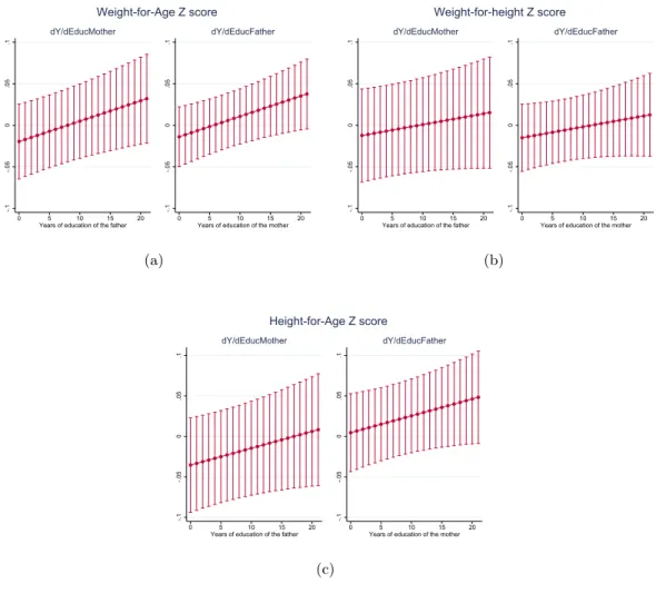
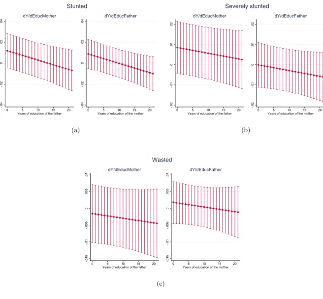
We here use the analytical sample to jointly estimate the effect of father’s and mother’s education and the interaction between them. The estimates from the four specifications are summarized in Tables 10-12. Given the interaction, the total effect of mother’s education on health depends on the father’s education when the interaction term is significantly different from zero ; the same holds for the total effect of father’s education. The total effect of mother’s and father’s education for any level of education of the other parent and the associated 95-percent confidence intervals are depicted in Figures 2-5 for the IV specification correcting for selection (column 4 of Tables 10-12). The estimated coefficients here can be compared to those in Table 9 from the same sample but without controlling for the presence of the father, in order to evaluate the bias in the previous estimates. The full results, showing the estimates on the control variables, the Inverse Mills ratios and the correlation between the unobservables are in Appendix Tables B2-B4.
The effects of education on prenatal care and birth outcomes : Overall, our findings on prenatal care and birth suggest that mother’s education has a mixed effect on the four outcomes, while father’s education consistently and significantly improves prenatal care and the presence of a skilled health assistant during birth (see Table 10 and Figure 2).
First, the number of prenatal visits significantly falls with mother’s education for low values of father’s education (when he has no education or only one year of schooling) and increases with mother’s education for high values of father’s education (17 years of schooling or more). However,