Serviceability and safety in the design of rigid inclusions and combined pile-raft foundations

(1)

HAL Id: tel-01259962

https://pastel.archives-ouvertes.fr/tel-01259962

Submitted on 21 Jan 2016

HAL is a multi-disciplinary open access

archive for the deposit and dissemination of sci-entific research documents, whether they are pub-lished or not. The documents may come from teaching and research institutions in France or

L’archive ouverte pluridisciplinaire HAL, est destinée au dépôt et à la diffusion de documents scientifiques de niveau recherche, publiés ou non, émanant des établissements d’enseignement et de recherche français ou étrangers, des laboratoires

and combined pile-raft foundations

Cecilia Bohn

To cite this version:

Cecilia Bohn. Serviceability and safety in the design of rigid inclusions and combined pile-raft founda-tions. Civil Engineering. Université Paris-Est, 2015. English. �NNT : 2015PESC1096�. �tel-01259962�

(2)

Serviceability and safety in the design of

rigid inclusions and combined pile-raft

foundations

Cécilia Bohn

PhD thesis in double degree programme, defended on the 30th September 2015 at the Technical University Darmstadt

Examination committee:

Prof. Matthias Becker (Technical University Darmstadt) President Prof. Eduardus Koenders (Technical University Darmstadt) Referee

Prof. Hussein Mroueh (Lille University) Referee

Prof. Norbert Vogt (Technical University Munich) Referee

Prof. Roger Frank (ENPC, University Paris-Est) PhD supervisor Prof. Rolf Katzenbach (Technical University Darmstadt) PhD co-supervisor Prof. Stefan Schäfer (Technical University Darmstadt) Additional examiner

(3)

First of all and above all, I would like to express my deepest gratitude to my PhD supervisor Prof. Roger Frank for giving the best supervision I could imagine for my thesis. It was an extraordinary combination of great scientific support, constant availability (despite ISSMGE presidency), and permanent confidence in me and in the directions I chose to give to my thesis. His warm understanding helped me a lot in the many difficult times I encountered organizing all double degree appointments. Roger, I will miss our discussion times in Paris! I would like to thank as well the members of the Navier-Geotechnics laboratory (Cermes) for immediately giving me the feeling that I am part of the team, even if I spent only few months there.

I wish to thank Prof. Rolf Katzenbach for accepting to co-supervise my thesis in this double degree programme. Thanks to the team of the Institute and Laboratory of Geotechnics of the Technical University Darmstadt for hosting me and for the experience I could gain in teaching activities there during the first year of my thesis.

I appreciated particularly the detailed reviewing of the referees, Prof. Eduardus Koenders, Prof. Hussein Mroueh and Prof. Norbert Vogt, who showed a great interest in my work. The very kind participation of Prof. Matthias Becker as president of the examination committee and of Prof. Stefan Schäfer completed perfectly the French-German examination committee. Special thanks go to Cécile Blanchemanche and Claudia Castrillon from both partner institutions for their efforts helping me organizing the double degree programme.

I would like to thank of course my supervisors of the company Keller Holding GmbH for developing this subject together with me and for supporting technically and financially this research from the beginning. I am very grateful to my colleagues of the EMEA Corporate Services team and of the Keller branch offices all over the world for the very motivating and pleasant work, helping me giving the right orientation of my research to make it as useful as possible for the engineering practice.

I would like to thank warmly Prof. Ulrich Trunk and Timo Ackermann for their particular dedication to our common work. Special thanks go to Alexandre Lopes dos Santos and Arefeh Rostami for their strong initiative carrying out useful analyses for my thesis during their internships within Keller. Many thanks go to Dorian Nogneng, Matthieu Appenzeller and Thomas Reichl as well for their valuable advice and support in programming. Thanks a lot to Sébastien Burlon, Sabrina Perlo, Michel Gambin and Olivier Combarieu for the pleasant exchanges and for the indispensable background they provided to me in foundation engineering and in the pressuremeter theory.

(4)

Contents

List of appendices IV

List of figures V

List of tables XVII

List of symbols and abbreviations XX

1 Introduction 1

2 State of the art and literature analysis 4

2.1 Design of shallow foundations according to Eurocode 7 4

2.1.1 Current practice in Germany 4

2.1.1.1 Bearing capacity 4

2.1.1.2 Settlement 6

2.1.2 Current practice in France 6

2.2 Design of pile foundations according to Eurocode 7 11

2.2.1 Current practice in Germany 11

2.2.2 Current practice in France 15

2.3 Pile groups 22

2.3.1 Principle and behaviour 22

2.3.2 Pile group system calculation 23

2.3.2.1 Empirical methods 23

2.3.2.2 Elastic continuum methods 24

2.3.2.3 Hybrid methods with load transfer curves 31

2.3.2.4 Continuum methods 33

2.4 Combined pile-raft foundations (CPRF) 34

2.4.2 CPRF system calculation 38

2.4.2.1 Elastic continuum methods 38

2.4.2.2 Analytical hybrid methods with load transfer curves 43

2.5 Rigid inclusions (RI) 49

2.5.2 RI system calculation 53

2.5.2.1 Simplified and equivalence methods 53

2.5.2.2 Load transfer method (LTM) with load transfer curves 55

2.6 Stone columns 62

(5)

2.6.2 Deformation parameters and settlement 64 2.7 Comparison of safety concepts for usual and combined foundation systems 67

2.7.1.1 Safety concept for RI after ASIRI (IREX 2012) 68

2.7.1.2 External bearing capacity (GEO) 70

2.7.1.3 Internal structural capacity (STR) 72

3 Investigation of the settlement of shallow foundations 74

3.1 Application of moduli correlations for linear elastic calculation 74

3.2 Single footing non-linear settlement behaviour 77

4 Investigation of the settlement of pile foundations 83

4.1 Pile load test database 83

4.2 Single pile axial behaviour with the FEM and moduli correlations 85 4.2.1 Need of relevant correlations for single pile loading 85 4.2.2 Example of moduli back-calculation for an instrumented single pile 88 4.3 Development of axial load transfer curves for LTM applications 97

4.3.1 Existing load transfer curves 97

4.3.2 Development of load transfer curves based on instrumented load tests 101

4.3.2.1 Analysis of existing curves 101

4.3.2.2 Proposal of new explicit curves 106

4.3.3 Validation based on non-instrumented load tests 111

5 Application of Load Transfer Method (LTM) to combined foundation systems 118 5.1 Load transfer method development for combined systems 118

5.1.1 General aspects 118

5.1.2 Large slabs or embankments: unit cell calculation 119

5.1.3 Single footings: oedometer and pressuremeter method 121 5.2 Comparison and transition between CPRF and RI systems based on reference

cases with measurements 124

5.2.1 Infinite grid system 124

5.2.1.1 Reference RI infinite grid case with measurements 124

5.2.1.2 Variation of load 129

5.2.1.3 Variation of LTP thickness 132

5.2.1.4 Comparison between rigid and flexible slab cases 134

5.2.2 Single footing system 137

5.2.2.1 Reference CPRF case with measurements 137

5.2.3 High-rise building example 144

5.2.3.1 Reference case with measurements 144

5.3 Comparison of LTM with FEM for theoretical single footing combined

(6)

5.3.1 General modelling aspects 156

5.3.2 Calibration on case without columns 162

5.3.3 Comparison in CPRF case 165

5.3.4 Comparison in RI case 171

6 Sensitivity investigation 182

6.1 Influence of column material in a unit cell system 182

6.1.2 Concrete column and stone column reference cases 185

6.1.3 Variation of column modulus and material type 188

6.2 Influence of geometrical imperfections on a single column 190

6.2.2 Diameter reduction over whole column length 194

6.2.3 Necking and bulging 197

6.2.4 Inclination 202

6.2.5 Curvature 208

6.2.6 Load eccentricity 214

6.3 Comparison and recommendations 217

6.3.1 Column material imperfections 217

6.3.2 Column geometrical imperfections 218

7 Summary and outlook 221

8 Zusammenfassung und Ausblick 226

9 Résumé et perspectives 231

(7)

List of appendices

Appendix A. Soil deformation parameters and settlement of usual foundations A.1 General aspects

A.2 Oedometer test A.3 Plate load test

A.4 Pressuremeter test (PMT)

Appendix B. Soil resistance parameters and bearing capacity of usual foundations B.1 Laboratory tests

B.2 Cone penetration test (CPT) B.3 Pressuremeter test (PMT)

Appendix C. Correlations between soil parameters C.1 CPT and PMT and other tests parameters C.2 CPT parameters and soil moduli

C.3 Different soil moduli

Appendix D. Main properties of pile load tests in database D.1 Instrumented non-displacement pile load tests

D.2 Instrumented displacement pile load tests

D.3 Non-instrumented non-displacement pile load tests (or considered as such) D.4 Non-instrumented displacement pile load tests (or considered as such)

(8)

List of figures

Fig. 1.1 Rigid inclusion (RI) system in comparison with usual foundation systems

from ASIRI (IREX 2012) 1

Fig. 2.1 Diagrams for factor kp for bearing capacity of shallow foundations after

NF P94-261 (2013) 9

Fig. 2.2 Load-settlement curve for bored piles after EA-Pfähle (DGGT 2012) 13 Fig. 2.3 Definition of fsol for ultimate skin friction translated from NF P94-262

(2012) 20

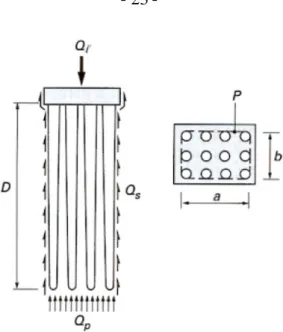
Fig. 2.4 Load transfer method for axially loaded piles 21

Fig. 2.5 Load transfer curves after Frank and Zhao (1982) for skin friction (left) and base resistance (right) after NF P94-262 (2012) 21 Fig. 2.6 Massive fictive pile for calculation of bearing capacity of pile groups

(Frank 1999) 23

Fig. 2.7 Pile group settlement for floating piles after Terzaghi method (Frank

1999) 24

Fig. 2.8 Shear stress distribution around the pile for single pile settlement after

Frank (1975) and Randolph (Mossallamy 1997) 25

Fig. 2.9 Superposition of settlement profiles for a pile group (Fleming et al. 2008) 26 Fig. 2.10 Linear elastic calculation for settlement of a single pile after Poulos

(1994), cited by Smoltczyk (2001): settlement factor Iρ vs. relative length

28 Fig. 2.11 Group interaction factors vs. relative spacing between two piles after

Poulos and Davis (1980), cited by Frank (1999) 29

Fig. 2.12 Group interaction factors between two piles (Viggiani et al. 2011) 30 Fig. 2.13 Charts for calculation of exponent e for pile group settlement (Fleming et

al. 1985) 31

Fig. 2.14 Skin friction displacement factor y for group effect with load transfer

curves 32

Fig. 2.15 Inclination reduction of skin friction load transfer curve for group effect

(Randolph 1994) 32

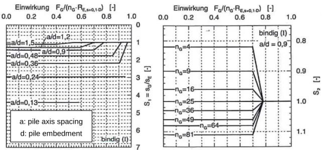
Fig. 2.16 Diagram for S1 and S2 vs. load level for cohesive soils (I) (EA-Pfähle,

DGGT 2012) 34

Fig. 2.17 Schematic design concept of shallow foundations (a), CPRFs (b) and deep

foundations (c) (Borel 2001) 35

Fig. 2.18 Interactions in CPRF system (Katzenbach and Choudhury 2013) 36 Fig. 2.19 Theoretically mobilised pile skin friction with and without loading of the

(9)

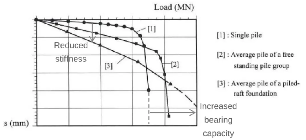
Fig. 2.20 Pile load-settlement behaviour: single pile, pile in a group, pile in a CPRF

adapted from El-Mossallamy (1997) 37

Fig. 2.21 Interaction between pile and raft foundation elements (Borel 2001) 39 Fig. 2.22 Settlement of pile-raft system vs. raft/pile diameter ratio compared to

single rigid pile in an elastic continuum after Poulos and Davis (1980),

cited by Borel (2001) 41

Fig. 2.23 Settlement of CPRF and pile group vs. relative pile spacing compared to single rigid pile in an elastic continuum from Butterfield and Banerjee

(1971), cited by Borel (2001) 42

Fig. 2.24 Combined boundary element and finite element method for CPRF

(El-Mossallamy 1996) 43

Fig. 2.25 Principle of a hybrid method for CPRF from Clancy and Randolph (1993),

cited by Borel (2001) 44

Fig. 2.26 Soil and pile settlement profiles with the LTM after Combarieu (1988a) 45 Fig. 2.27 3D-modelling of CPRF-subsystem using symmetrical properties (Hanisch

et al. 2002) 46

Fig. 2.28 Full 3D-modelling of CPRF-system (Skyper-Tower in Frankfurt am Main)

(Richter and Lutz 2010) 46

Fig. 2.29 Increasing modulus with depth for FEM-modelling (Richter and Lutz

2010) 47

Fig. 2.30 Predesign-diagrams for a CPRF in theoretically infinitely deep Frankfurt clay (Reul 2000): settlement vs. number of piles and pile length 48 Fig. 2.31 Predesign-diagram for a CPRF in the Frankfurt clay with finite depth

(Reul 2000): settlement relatively to the case with infinite clay depth vs.

relative clay depth 49

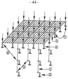
Fig. 2.32 Rigid inclusion (RI) application cases adapted from ASIRI (IREX 2012) 50 Fig. 2.33 Settlement, load-transfer behaviour and planes with equal settlements in

RI grid 51

Fig. 2.34 Influence of LTP thickness and slab rigidity on efficiency and settlement

behaviour adapted from (Höppner 2011) 52

Fig. 2.35 Equivalent raft settlement calculation for groups of rigid columns

(CSV-guideline, DGGT 2002) 54

Fig. 2.36 RI system as interpolation between unimproved footing and CPRF from

ASIRI (IREX 2012) 55

Fig. 2.37 Equivalent modulus Eoe for equivalent raft calculation (Combarieu 1990)

55 Fig. 2.38 Unit cell RI system for calculation with mobilisation functions adapted

from ASIRI (IREX 2012) 56

Fig. 2.39 Development of shear along the fictive columns to model the arching

(10)

Fig. 2.40 Load in the soil at the top of the columns after Combarieu from ASIRI

(IREX 2012) 58

Fig. 2.41 Prandtl’s failure mechanism for the compatibility check in the LTP after

ASIRI (IREX 2012) 59

Fig. 2.42 Diagram with domain of allowable stresses in LTP, adapted from ASIRI

(IREX 2012) 59

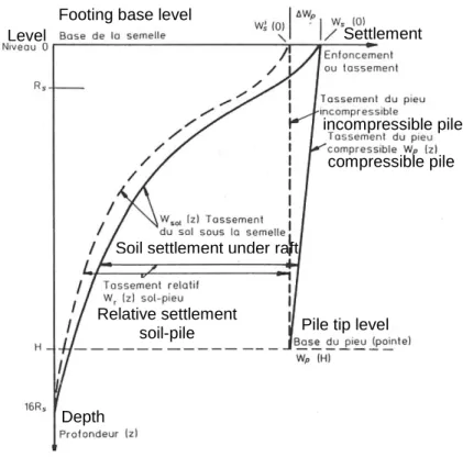
Fig. 2.43 Soil settlement profile under footing for calculation with load transfer

curves from ASIRI (IREX 2012) 60

Fig. 2.44 Steps for hybrid monolith method for RIs under footing (IREX 2012) 61 Fig. 2.45 Deformation of stone columns under service loads (Kirsch 2004) 63 Fig. 2.46 Failure mechanisms for stone columns from Datye (1982), cited by Soyez

(1985) 64

Fig. 2.47 Elastic calculation method for compressible piles from Mattes and Poulos (1969), cited by Soyez (1985): settlement factor Iρ vs. column/soil

stiffness ratio 65

Fig. 2.48 Settlement relatively to unimproved settlement vs. stone columns spacing

after Greenwood (1970) 65

Fig. 2.49 Comparison of settlement calculation methods for stone columns (Greenwood and Kirsch 1983): settlement reduction ratio vs. area ratio 67 Fig. 2.50 Check of geotechnical capacity of single columns in function of column

diameter according to standards and recommendations 71 Fig. 3.1 Example site with in situ soil tests for settlement calculation of shallow

foundations 74

Fig. 3.2 Example site: soil configuration and shallow foundation cases 75 Fig. 3.3 Proposal of Combarieu (1988a) for footing load-settlement curve

(spherical and deviatoric components) 78

Fig. 3.4 Proposal of Briaud (2007) for footing load-settlement curve 78 Fig. 3.5 Measured and modelled footing load-settlement curves 81 Fig. 3.6 Proposed hyperbolic mobilisation curve for single footing resistance 82 Fig. 4.1 Example of pile instrumentation with the “removable extensometer”

system 84

Fig. 4.2 Main results of an instrumented load test with “removable extensometer”. Left: load-settlement curve for head and tip; Middle: shaft load distribution between blockers and extrapolation for tip load; Right: skin

friction load transfer curve 84

Fig. 4.3 Stress path of soil around axially loaded single pile in comparison with

usual tests and shallow foundations 86

Fig. 4.4 Comparison of modulus ranges from usual correlations for different

foundation types for clay and sand 87

Fig. 4.5 Definition of E50 from deviatoric stress vs. axial strain diagram (Plaxis

(11)

Fig. 4.6 2D-FEM-model of single pile Ifsttar 35 B (layers with main parameters,

pile, interfaces and mesh) 91

Fig. 4.7 Comparison of measured mobilisation curve of skin friction in the third layer with the back-calculated FEM model and with the Frank and Zhao (1982) prediction (instrumented load test Ifsttar 35B) 92 Fig. 4.8 Measured and modelled load-settlement curve after back-calculation at

pile head and at pile tip (instrumented load test Ifsttar 35B) 93 Fig. 4.9 Measured and modelled load in pile with depth (instrumented load test

Ifsttar 35B) 94

Fig. 4.10 Comparison of back-calculated moduli in each layer of the FEM model with usual correlations (instrumented load test Ifsttar 35B) 95 Fig. 4.11 Stress paths of stress point at the interface half way down the second layer

and of stress point directly under the pile tip in the FEM model

(instrumented load test Ifsttar 35B) 96

Fig. 4.12 Example of level of agreement of predicted load transfer curves 102 Fig. 4.13 Percentage of measured skin friction curves with peaks for different soil

and pile types 103

Fig. 4.14 Variability in measured and modelled peak behaviours 103 Fig. 4.15 Level of agreement of the existing load transfer curves 104 Fig. 4.16 Level of agreement of the existing load transfer curves for the initial

stiffness 104

Fig. 4.17 Example of calibration of cubic root curves at shaft and at tip 106 Fig. 4.18 Cubic root curves  Calibration of limit settlements ss,lim and sb,lim 107

Fig. 4.19 Limit settlements ss,lim and sb,lim in function of CPT cone resistance for

cubic root curves (qc = 0 MPa means no CPT data) 107

Fig. 4.20 Example of calibration of hyperbolic curve at shaft and at tip 109 Fig. 4.21 Hyperbolic curves  Calibration of parameters Ms and Mb 110

Fig. 4.22 Shaft parameter Ms and tip parameter Mb in function of cone resistance for

hyperbolic curves (qc = 0 MPa means no CPT data) 110

Fig. 4.23 Level of agreement of the proposed load transfer curves compared with Frank and Zhao curves (global agreement and initial stiffness) 111 Fig. 4.24 LTM single column system with required input parameters 112 Fig. 4.25 Example of a single pile analysis with test Ifsttar 1-A1 under a given load

with the LTM: output under 1000 kN 113

Fig. 4.26 Example of a single pile analysis with test Ifsttar 1-A1 with the LTM: load-settlement curve and load distribution along the shaft for different

loads 114

Fig. 4.27 Examples of comparison between measured and predicted load-settlement

curves at pile head 115

Fig. 4.28 Ratio between predicted and measured settlement for both proposed load

(12)

Fig. 5.1 Unit cell for large slabs or embankments with required input parameters 119 Fig. 5.2 System for calculation of slab bending moments m after plate theory 121 Fig. 5.3 Soil settlement profile under a single footing according to the

pressuremeter theory (Combarieu 1988a) 123

Fig. 5.4 LTM Single footing with oedometer method or pressuremeter method

with required input parameters 123

Fig. 5.5 Cross section of monitored RI field test for ASIRI in Saint-Ouen-l’Aumône with main soil and foundation parameters (Briançon and Simon

2010) 125

Fig. 5.6 Results of LTM calculation of infinite grid system of the ASIRI field test with a rigid slab with Frank and Zhao load transfer curves 126 Fig. 5.7 Results of LTM calculation of infinite grid system of the ASIRI field test

with a rigid slab with proposed cubic root load transfer curves 127 Fig. 5.8 Results of LTM calculation of infinite grid system of the ASIRI field test

with a rigid slab with proposed hyperbolic load transfer curves 127 Fig. 5.9 Results of LTM calculation of infinite grid system of the ASIRI field test

with a flexible slab with Frank and Zhao load transfer curves 128 Fig. 5.10 Differential settlement measured in central unit cell of ASIRI field test

(Briançon and Simon 2010) 129

Fig. 5.11 Surface load-settlement based on ASIRI reference case with Frank and Zhao load transfer curves (infinite grid, rigid loading) 130 Fig. 5.12 Column load share vs. area load based on ASIRI reference case with

Frank and Zhao load transfer curves (infinite grid, rigid loading) 130 Fig. 5.13 Neutral plane variations vs. area load based on ASIRI reference case with

Frank and Zhao load transfer curves (infinite grid, rigid loading) 131 Fig. 5.14 Load-settlement behaviour based on ASIRI reference case with Frank and

Zhao load transfer curves (infinite grid, rigid loading) compared to single

column case 132

Fig. 5.15 Settlement at the top vs. LTP thickness based on ASIRI reference case with Frank and Zhao load transfer curves (infinite grid, rigid loading) 133 Fig. 5.16 Column load share vs. LTP thickness based on ASIRI reference case with

Frank and Zhao load transfer curves (infinite grid, rigid loading) 133 Fig. 5.17 Neutral plane variations vs. LTP thickness based on ASIRI reference case

with Frank and Zhao load transfer curves (infinite grid, rigid loading) 134 Fig. 5.18 Settlement at the top vs. LTP thickness based on ASIRI reference case

with Frank and Zhao load transfer curves (infinite grid, rigid and flexible

loading) 135

Fig. 5.19 Column load share vs. LTP thickness based on ASIRI reference case with Frank and Zhao load transfer curves (infinite grid, rigid and flexible

(13)

Fig. 5.20 Neutral plane variations vs. LTP thickness based on ASIRI reference case with Frank and Zhao load transfer curves (infinite grid, rigid and flexible

loading) 136

Fig. 5.21 Bending moment at the edge and at the centre of the unit cell based on ASIRI reference case with Frank and Zhao load transfer curves (infinite

grid, rigid loading) 137

Fig. 5.22 Test site picture and cross section of monitored CPRF field test in

Merville (Borel 2001) 138

Fig. 5.23 Settlement with load in CPRF field test from Borel (2001): measurements and predictions with FONMIX and with proposed LTM calculation 140 Fig. 5.24 Pile load share with load in CPRF field test from Borel (2001):

measurements and predictions with FONMIX and with proposed LTM

calculation 140

Fig. 5.25 Results of LTM calculation of CPRF with rigid footing field test from Borel (2001) with Frank and Zhao load transfer curves for intermediate

load level of 1091 kN 141

Fig. 5.26 Load-settlement behaviour based on Borel (2001) reference case: with Frank and Zhao load transfer curves compared to single column case 142 Fig. 5.27 Settlement at the top vs. LTP thickness based on Borel (2001) reference

case with Frank and Zhao load transfer curves (rigid footing) 143 Fig. 5.28 Column load share vs. LTP thickness based on Borel (2001) reference

case with Frank and Zhao load transfer curves (rigid footing) 143 Fig. 5.29 Neutral plane variations vs. LTP thickness based on Borel (2001)

reference case with Frank and Zhao load transfer curves (rigid footing) 143 Fig. 5.30 Distribution of the soil modulus of oedometer type of the Frankfurt clay

evaluated from pressuremeter tests along the depth z (Reul 2000) 145 Fig. 5.31 Simplified distribution of Young’s modulus compared to pressuremeter

reloading modulus (Reul 2000) 145

Fig. 5.32 Vertical cross section and plan view of monitored CPRF foundation of high-rise building Westend 1 in Frankfurt (Reul 2000) 146 Fig. 5.33 Pile load vs. settlement for different pile locations for CPRF Westend 1

(Reul 2000) 147

Fig. 5.34 Results of LTM calculation of CPRF Westend 1 as infinite grid system with a rigid slab with cubic root load transfer curves 149 Fig. 5.35 Results of LTM calculation of CPRF Westend 1 as infinite grid system

with a rigid slab with hyperbolic load transfer curves 149 Fig. 5.36 Results of LTM calculation of CPRF Westend 1 as infinite grid system

with a rigid slab with Frank and Zhao load transfer curves 150 Fig. 5.37 Measured settlement distribution along the depth of CPRF Westend 1

(14)

Fig. 5.38 Settlement at the top vs. load based on Westend 1 reference case with cubic root and hyperbolic load transfer curves (infinite grid, rigid loading)

152 Fig. 5.39 Settlement share below pile tip vs. load based on Westend 1 reference case

with cubic root and hyperbolic load transfer curves (infinite grid, rigid

loading) 152

Fig. 5.40 Pile load share vs. load based on Westend 1 reference case with cubic root and hyperbolic load transfer curves (infinite grid, rigid loading) 153 Fig. 5.41 Load-settlement behaviour based on Westend 1 reference case: with cubic

root load transfer curves (infinite grid, rigid loading) compared to single

column case 154

Fig. 5.42 Settlement at the top vs. LTP thickness based on Westend 1 reference case with cubic root and hyperbolic load transfer curves (rigid loading) 155 Fig. 5.43 Column load share vs. LTP thickness based on Westend 1 reference case

with cubic root and hyperbolic load transfer curves (rigid loading) 155 Fig. 5.44 Neutral plane variations vs. LTP thickness based on Westend 1 reference

case with cubic root and hyperbolic load transfer curves (rigid loading) 155 Fig. 5.45 Bending moment at the edge and at the centre of the unit cell based on

Westend 1 reference case with cubic root and hyperbolic load transfer

curves (rigid loading) 156

Fig. 5.46 Plan view of footing with columns and position of sections A-A and B-B 157 Fig. 5.47 Mohr-Coulomb failure criterion for modelled concrete 158

Fig. 5.48 3D FEM model of footing without columns 159

Fig. 5.49 3D FEM model of footing with columns without LTP 160

Fig. 5.50 3D FEM model of footing with columns with LTP 161

Fig. 5.51 Footing load-settlement curves with 3D FEM and LTM 162 Fig. 5.52 Vertical stresses over bottom surface of the footing with 3D FEM for case

without columns 163

Fig. 5.53 Profiles of vertical stress due to load with 3D FEM and LTM without

columns 164

Fig. 5.54 Settlement profiles with 3D FEM and LTM without columns 164 Fig. 5.55 Vertical stresses over bottom surface of the footing with 3D FEM for

CPRF case (right: only soil stresses; in Plaxis: compression negative) 165 Fig. 5.56 Vertical stresses in section A-A (see Fig. 5.46) with 3D FEM for CPRF

case (in Plaxis: compression negative) 166

Fig. 5.57 Vertical stresses in section B-B (see Fig. 5.46) with 3D FEM for CPRF case (left: only column stresses; right: only soil stresses; in Plaxis:

compression negative) 166

Fig. 5.58 Vertical displacement in section A-A (see Fig. 5.46) with 3D FEM for

(15)

Fig. 5.59 Vertical displacement in section B-B (see Fig. 5.46) with 3D FEM for

CPRF case 167

Fig. 5.60 Comparison of LTM and 3D FEM results for CPRF case: settlement and skin friction mobilisation (depth 0 m: column head position) 169 Fig. 5.61 Comparison of LTM and 3D FEM results for CPRF case: additional stress

in the column and in the soil due to the load applied (depth 0 m: column

head position) 170

Fig. 5.62 Footing load-settlement curve in CPRF with 3D FEM compared with

load-settlement curves without columns 171

Fig. 5.63 Failure points in LTP (RI case) with 3D FEM (left: in section A-A; right:

section B-B after Fig. 5.46) 172

Fig. 5.64 Vertical stresses over bottom surface of the footing with 3D FEM for RI

case (in Plaxis: compression negative) 173

Fig. 5.65 Vertical stresses in section A-A (see Fig. 5.46) with 3D FEM for RI case

(in Plaxis: compression negative) 173

Fig. 5.66 Vertical stresses in section B-B (see Fig. 5.46) with 3D FEM for RI case (left: only column stresses; right: only soil stresses; in Plaxis: compression

negative) 174

Fig. 5.67 Detail of vertical stresses in LTP in section B-B (see Fig. 5.46) with 3D FEM for RI case (in Plaxis: compression negative) 174 Fig. 5.68 Skin friction mobilisation with 3D FEM for RI case 175 Fig. 5.69 Vertical displacement over bottom surface of the footing with 3D FEM for

RI case 176

Fig. 5.70 Vertical displacement in section A-A (see Fig. 5.46) with 3D FEM for RI

case 176

Fig. 5.71 Vertical displacement in section B-B (see Fig. 5.46) with 3D FEM for RI

case 177

Fig. 5.72 Directions of principal stresses in section B-B (see Fig. 5.46) with 3D

FEM for RI case 177

Fig. 5.73 Comparison of LTM and 3D FEM results on RI case: settlement and skin friction mobilisation (depth 0 m: column head position) 179 Fig. 5.74 Comparison of LTM and 3D FEM results in RI case: additional stress in

the column and in the soil due to the load applied (depth 0 m: column head

position) 181

Fig. 6.1 Axisymmetric FEM-model for column material variation (layers with

main parameters and mesh) 183

Fig. 6.2 Young’s modulus vs. compressive strength for usual concrete and

lightweight concrete 184

Fig. 6.3 Comparison of vertical stresses between concrete column and stone column reference cases (in Plaxis: compression negative) 186

(16)

Fig. 6.4 Comparison of horizontal deformations between concrete column and

stone column reference cases 187

Fig. 6.5 Comparison of failure points between concrete column and stone column

reference cases 187

Fig. 6.6 Bending moments in the plate vs. distance to centre of the unit cell for the concrete column and for the stone column reference cases 188 Fig. 6.7 Settlement at the top vs. modulus ratio column to soil for bonded and

coarse-grained column (Eoed,soilref = 6.5 MPa) 189

Fig. 6.8 Settlement at the LTP base level vs. modulus ratio column to soil for bonded and coarse-grained column (Eoed,soilref = 6.5 MPa) 189

Fig. 6.9 Column load share at the column head vs. modulus ratio column to soil for bonded and coarse-grained column (Eoed,soilref = 6.5 MPa) 190

Fig. 6.10 Reference single column for analytical study 192

Fig. 6.11 Single column axisymmetric FEM reference model 193

Fig. 6.12 Diameter imperfection for analytical study 195

Fig. 6.13 Loss of resistance due to diameter variation over whole height from

analytical study 195

Fig. 6.14 Load-settlement curves for different diameters from axisymmetric FEM

analysis 196

Fig. 6.15 Loss of bearing capacity due to a diameter reduction of 10 cm from axisymmetric FEM analysis compared to analytical results 197 Fig. 6.16 Settlement increase under service load due to a diameter reduction of

10 cm from FEM analysis 197

Fig. 6.17 Necking and bulging imperfection for axisymmetric FEM analysis 198 Fig. 6.18 Vertical stress in necking zone from axisymmetric FEM analysis for

B = 30 cm 199

Fig. 6.19 Load-settlement curves with bulging and necking from axisymmetric FEM

analysis for B = 30 cm 200

Fig. 6.20 Directions of principal stresses in the soil with bulging and necking from

axisymmetric FEM analysis for B = 30 cm 201

Fig. 6.21 Increase of bearing capacity with bulging and necking from axisymmetric

FEM analysis 201

Fig. 6.22 Inclination imperfection with parameters for analytical study 202 Fig. 6.23 Load section vs. normalized lever arm from analytical study 204

Fig. 6.24 Inclination imperfection for 3D FEM analysis 204

Fig. 6.25 Load-settlement curves with column inclination from 3D FEM analysis

for B = 30 cm 205

Fig. 6.26 Normal stress in the interface around the inclined columns under the maximum applied load from 3D FEM analysis for B = 30 cm 206 Fig. 6.27 Skin friction in the interface around the inclined columns under the

(17)

Fig. 6.28 Vertical stress (in Plaxis: compression negative) and bending moment in the inclined column from 3D FEM analysis for B = 30 cm 207 Fig. 6.29 Curvature imperfection with parameters for analytical study 209 Fig. 6.30 Buckling load and geotechnical bearing capacity in function of curvature

imperfection for B = 30 cm 210

Fig. 6.31 Stresses in section in function of curvature imperfection for service load of

189 kN (half of bearing capacity) for B = 30 cm 211

Fig. 6.32 Curvature for 3D FEM analysis 211

Fig. 6.33 Load-settlement curves with column curvature from 3D FEM analysis for

B = 30 cm 212

Fig. 6.34 Vertical stress in the curved column from 3D FEM analysis for B = 30 cm

(in Plaxis: compression negative) 213

Fig. 6.35 Load eccentricity for analytical study 214

Fig. 6.36 Load eccentricity for 3D FEM analysis 215

Fig. 6.37 Load-settlement curves with load eccentricity from 3D FEM analysis for

B = 30 cm 216

Fig. 6.38 Vertical stress at the top of the eccentric-loaded column from 3D FEM analysis for B = 30 cm (in Plaxis: compression negative) 216 Fig. A.1 Compression uni-axial test on elastic material (Combarieu 2006) 262 Fig. A.2 Compression tri-axial test on elastic material and on soil (Briaud 2000) 263 Fig. A.3 Different slopes in stress-strain curve, adapted from (Briaud 2000) 264 Fig. A.4 Modulus vs. amplitude of deformations (Ménard 1961) 265 Fig. A.5 Different initial slopes for different confinement level in tri-axial tests

(Katzenbach, lecture notes 2015) 266

Fig. A.6 Shear modulus depending on shear strain and loading direction in

hypoplastic model (Kudella and Reul 2002) 267

Fig. A.7 Oedometer test (Katzenbach, lecture notes 2015) 267

Fig. A.8 Deformation of soil element under large and limited loading area

(Baguelin et al. 1978) 268

Fig. A.9 Stress-strain curve in oedometer test (non-linearity) 269 Fig. A.10 Influence of the nature of stress field on stress-strain relationship (Ménard

1961) 269

Fig. A.11 Void ratio vs. applied stress in logarithmic scale curve in oedometer test

(adapted from Combarieu 2006) 270

Fig. A.12 Load distribution and segmentation for oedometric settlement method under shallow foundations (Philipponnat and Hubert 2000) 271 Fig. A.13 Corrective factor μ to take into account the tridimensional effects after

Skempton and Bjerrum (1957), cited by Frank (1999) 272

Fig. A.14 Plate load test – Westergaard type (Cassan 1988) 274

(18)

Fig. A.16 Pressuremeter testing on test field of Navier-Géotechnique (Cermes) in

Lognes, France 276

Fig. A.17 Main components of a pressuremeter unit (Gambin 2005) 277

Fig. A.18 Shape of a pressuremeter curve (Cassan 1988) 277

Fig. A.19 Corrected pressuremeter curves with different phases (Ménard and

Rousseau 1962) 279

Fig. A.20 Ratio between oedometer modulus and dynamic modulus (Smoltczyk

2001) 279

Fig. A.21 Deformation of an initial square ring element for the cylindrical cavity

expansion (Baguelin et al. 1978) 280

Fig. A.22 Distortion in simple-shear test (Combarieu 2006) 280

Fig. A.23 Evolution of shear modulus with distortion (Combarieu 2006) 281 Fig. A.24 Circular foundation with zone of spherical and deviatoric stresses (Ménard

and Rousseau 1962) 286

Fig. A.25 Increase of the settlement in case of small embedment (Baguelin et al.

1978) 288

Fig. A.26 Subdivision in layers of thickness B/2 for equivalent modulus 289 Fig. A.27 Stress and strains along a vertical axis under a rigid circular foundation

(elastic) (Baguelin et al. 1978) 290

Fig. A.28 Original transfer functions by Frank and Zhao for skin friction (top) and tip resistance (bottom) for fine-grained soils (Frank and Zhao 1982) and

(Frank 1985) 291

Fig. B.1 Failure mechanism under a shallow foundation after Prandtl (Frank 1999) 293 Fig. B.2 Possible failure mechanism under a pile foundation for the methods based

on soil shear parameters (Frank 1999) 294

Fig. B.3 Example of a tip of a CPT testing probe after EN ISO 22476-1 (2012) 295 Fig. B.4 1) Pressuremeter curve, 2) Creep pressuremeter curve (Gambin 2005) 297 Fig. B.5 Example of creep pressuremeter curve (Baguelin et al. 1978) 297 Fig. B.6 Constitutive models for soils -1) real elastic-plastic response, 2) elastic

response without failure, 3) plastic rigid response, 4) simplified

elastic-plastic model (Gambin 1979) 299

Fig. B.7 Different mobilisation levels of soil strength around foundation base

(Ménard 1963a) 300

Fig. B.8 Distribution of stress isostatic lines around foundation base (Ménard 1963) 300 Fig. B.9 Bearing capacity versus depth of embedment (Ménard 1963a) 301 Fig. B.10 Plastic failure zones under shallow and deep foundation (Gambin 1979) 302 Fig. C.1 Measurements of EM, pl and qc for sand by Nazaret (Baguelin et al. 1978)

(19)

Fig. C.2 Ratio kq between qc and pLS for sands of different densities ID* (Cudmani

and Osinov 2001) 306

Fig. C.3 pLC (= pl) and pLS for different sands, different p0 and different ID

(Cudmani 2001) 307

Fig. C.4 Correlation between qc (CPT), pl (PMT) and N (SPT) (Bustamante and

Gianeselli 2006) 308

Fig. C.5 Roberston’s diagrams after NF P94-261 (2013) 312

Fig. C.6 Estimation of equivalent Young’s modulus for sand based on degree of

(20)

List of tables

Table 2.1 Indicative values for bearing capacity of shallow foundations in coarse-grained soils in Germany translated from DIN 1054 (2010) 5 Table 2.2 Indicative values for bearing capacity of shallow foundations in clay in

Germany translated from DIN 1054 (2010) 6

Table 2.3 Table for factor kp for bearing capacity of shallow foundations translated

from NF P94-261 (2013) 9

Table 2.4 Rheological factor α for different soil types and different ranges of EM/pl

translated from NF P94-261 (2013) 10

Table 2.5 Shape factors λc and λd for different soil types and different ranges of

EM/pl translated from NF P94-261 (2013) 11

Table 2.6 Tip resistance for bored piles in coarse-grained soils translated from

EA-Pfähle (DGGT 2012) 14

Table 2.7 Tip resistance for bored piles in fine-grained soils translated from

Table 2.8 Ultimate skin friction for bored piles in coarse-grained soils translated

from EA-Pfähle (DGGT 2012) 14

Table 2.9 Ultimate skin friction for bored piles in fine-grained soils translated from

Table 2.10 Ultimate skin friction for bored piles in rock translated from EA-Pfähle

(DGGT 2012) 15

Table 2.11 Definition of classes of piles translated from NF P94-262 (2012) 17 Table 2.12 Table for kpmax factor for pile base resistance translated from NF P94-262

(2012) 18

Table 2.13 Table of factor αpieu-sol for ultimate skin friction translated from NF

P94-262 (2012) 19

Table 2.14 Summary of prevalent settlement calculation methods for stone columns

(Kirsch 2004) 66

Table 2.15 Chart of safety checks after ASIRI (IREX 2012) 69

Table 2.16 Partial resistance safety factors – ASIRI ULS-GEO 70 Table 2.17 Partial resistance safety factors – Eurocode 7 ULS-GEO 70 Table 2.18 Partial resistance safety factors – CPRF and CSV-guidelines ULS-GEO 71 Table 2.19 Partial resistance safety factors – ASIRI SLS-GEO 72 Table 2.20 Partial resistance safety factors – Eurocode 7 SLS-GEO 72 Table 2.21 Partial resistance safety factors – CPRF and CSV-guidelines SLS-GEO 72 Table 3.1 Example site: comparison of settlement calculation methods for shallow

foundations and modulus calibration 76

(21)

Table 4.2 Pile load tests used for checking of developed load transfer curves (mainly

non-instrumented) 85

Table 4.3 Comparison of calculation methods and oedometer modulus ranges from usual correlations for different foundation types in clay and sand 87 Table 4.4 Results of PMT and of CPT near the Ifsttar 35 B test pile 94 Table 4.5 Definition of the main simple load transfer curves (1/2) 99 Table 4.6 Definition of the main simple load transfer curves (continued, 2/2) 100

Table 4.7 Proposed cubic root load transfer curves 106

Table 4.8 Proposed hyperbolic load transfer curves 109

Table 4.9 Example of a single pile analysis with test Ifsttar 1-A1 under a given load

with the LTM: input parameters 113

Table 5.1 LTM parameters for infinite grid system of the ASIRI field test 126 Table 5.2 Comparison of measurements with predictions for the ASIRI field test 129 Table 5.3 LTM parameters for CPRF with rigid footing field test in Merville after

FONMIX calculation by Borel (2001) 139

Table 5.4 LTM parameters for CPRF Westend 1 as infinite rigid slab 148 Table 5.5 Comparison of measurements with predictions for the CPRF Westend 1 151

Table 5.6 LTM parameters for CPRF case 168

Table 5.7 LTM parameters for RI case 178

Table 6.1 Stress level at the corner of the necking for different planned diameters and necking position from axisymmetric FEM analysis 199 Table 6.2 Stresses at the edge of the column section for different diameters,

settlement levels and inclination imperfections from 3D FEM analysis 208 Table 6.3 Stresses at the edge of the column section for different diameters,

settlement levels and curvatures from 3D FEM analysis 213 Table 6.4 Stresses at the edge of the column section for different diameters,

settlement levels and load eccentricities from 3D FEM analysis 217 Table 6.5 Influence of column material type and modulus according to the present

study and to the published results 218

Table 6.6 Existing tolerances and recommendations for geometrical imperfections 220 Table A.1 Usual values of EM for different types of soils (Techniques Louis Ménard

1975) 282

Table A.2 Rheological factor α for various soils (Baguelin et al. 1978) 284 Table B.1 Usual values of pl for different types of soils (Ménard 1975) 298

Table C.1 Ratio spans qc/pl for clay, silt and sand (Techniques Louis Ménard 1975)

304 Table C.2 Correlations between PMT and CPT parameters (Cassan 1988) 305 Table C.3 qc*/pl* for different soil types according to Baguelin et al. (1978) in

(22)

Table C.4 Correlations between PMT and CPT according to Briaud et al. (1985) in

(Hamidi et al. 2011) 308

Table C.5 Correlations between usual in situ parameters (internal document Keller

France) 309

Table C.6 Indicative ratio α to determine the oedometric modulus Eoed from the cone

resistance qc after EN 1997-2 (2007-2010) (based on Sanglerat 1972) 310

Table C.7 Indicative correlations values αfooting = E/EM for a single footing loading

case under serviceability loads from NF P94-261 (2013) 314 Table C.8 Comparison of moduli for equality of Ménard settlement method and

(23)

List of symbols and abbreviations

Abbreviations

CPRF combined pile-raft foundation

CPT cone penetration test

FEM finite element method

LTP load transfer platform

LTM load transfer method

PMT pressuremeter test

RI rigid inclusion system

SLS serviceability limite state in EN 1997-1 (2004-2009-2013) ULS ultimate limite state in EN 1997-1 (2004-2009-2013)

Symbols

Symbols defined differently or used only very locally (in particular from the literature) are defined in the text.

A foundation surface

Ab pile tip surface

B foundation width (for piles: pile diameter)

B0 reference foundation width in NF P94-261 (2013)

c soil cohesion

cu undrained shear strength

CC compression index in oedometer test

CS swelling index in oedometer test

D foundation embedment (for piles: pile length)

e eccentricity (alternatively: void ratio)

E Young’s modulus

E* calculation modulus after DIN 4019 (2015) (alternatively: equivalent oedometric modulus in ASIRI, IREX 2012)

Ec pressuremeter modulus of first layer under the foundation in

pressuremeter theory

Ed weighted pressuremeter modulus of layers under the foundation in

pressuremeter theory

Eoed constrained modulus (oedometer modulus)

EM pressuremeter modulus

(24)

EV plate load test modulus

E50 secant modulus in tri-axial test in Hardening Soil Model (Plaxis

2013, Plaxis 2014)

fc concrete compressive strength in EN 1992-1-1 (2004-2010)

Fc axial compression load on a pile in EN 1997-1 (2004-2009-2013)

G shear modulus

h or H layer thickness

kc cone penetration bearing factor in NF P94-261 (2013) and in

NF P94-262 (2012)

kp pressuremeter bearing factor in NF P94-261 (2013) and in

NF P94-262 (2012)

K0 earth pressure at rest

L foundation length

lm linear meter (or running meter)

m exponent for soil modulus definition in Hardening Soil Model (Plaxis 2013, Plaxis 2014)

Ms stiffness parameter of skin friction hyperbolic load transfer curve

Mb stiffness parameter of tip resistance hyperbolic load transfer curve

p’ mean effective stress

pl limit pressure in pressuremeter test

pref reference stress for soil modulus definition in Hardening Soil

Model (Plaxis 2013, Plaxis 2014)

q deviatoric stress

qb mobilised tip resistance (alternatively: ultimate tip resistance in

EN 1997-1 2004-2009-2013)

qc cone resistance from cone penetration test

qnet net bearing pressure resistance in NF P94-261 (2013)

qs mobilised skin friction (alternatively: ultimate skin friction in

EN 1997-1 2004-2009-2013)

qb,ult ultimate pile tip resistance

qs,ult ultimate pile skin friction

Q footing load

Qult footing ultimate load

R0 soil weight over the foundation area between the original ground

level and the foundation level in NF P94-261 (2013)

r radius

R bearing resistance in EN 1997-1 (2004-2009-2013)

Rc compressive ultimate pile resistance in EN 1997-1

(2004-2009-2013)

Rv net bearing resistance in NF P94-261 (2013)

(25)

sb pile tip settlement minus soil settlement in absence of the pile

sb,lim limit settlement for tip resistance cubic root curve

sc spherical component of the footing settlement in pressuremeter

theory

sd deviatoric component of the footing settlement in pressuremeter

theory

ss pile shaft settlement minus soil settlement in absence of the pile

ssg limit settlement in EA-Pfähle (DGGT 2012)

ssoil soil settlement

ss,lim limit settlement for skin friction cubic root curve

V vertical load on a foundation in EN 1997-1 (2004-2009-2013)

z depth

α structural or rheological factor in pressuremeter theory (alternatively: cone penetration test correlation factor in EN 1997-2 2007-2010)

αfooting correlation factor between pressuremeter modulus and Young’s

modulus for footing loading case

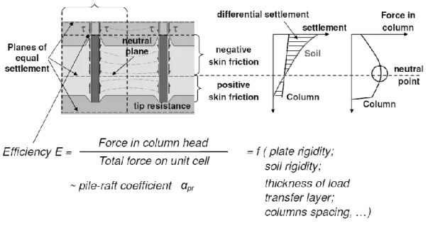
αpr pile-raft coefficient in CPRF-guideline (Katzenbach and

Choudhury 2013)

ε strain

 soil friction angle (alternatively: concrete creep factor in EN 1997-1 2004-2009-2013)

γ unit weight (alternatively: distortion)

γb partial factor for pile base (or tip) resistance in EN 1997-1

(2004-2009-2013)

γF partial factor for an action in EN 1997-1 (2004-2009-2013)

γG partial factor for a permanent action in EN 1997-1

(2004-2009-2013)

γQ partial factor for a variable action in EN 1997-1

(2004-2009-2013)

γR;v partial factor for bearing resistance in EN 1997-1

(2004-2009-2013)

γR;d;v model factor for bearing resistance in NF P94-261 (2013)

γR;d1 first model factor for pile resistance in NF P94-262 (2012)

γR;d2 first model factor for pile resistance in NF P94-262 (2012)

γs partial factor for pile shaft (or skin) friction resistance in

EN 1997-1 (2004-2009-2013)

λexp calibration parameter of exponential footing mobilisation curve

λhyp calibration parameter of hyperbolic footing mobilisation curve

ν Poisson’s ratio

(26)

σ stress

σR bearing pressure resistance in DIN 1054 (2010)

(27)

1 Introduction

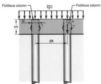
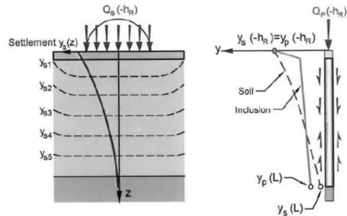
For given load levels, shallow foundations are acceptable foundations only for soils with sufficient stiffness and bearing capacity. If the load from the structures would lead to a ground failure or to excessive settlements, the use of deep foundations or soil reinforcements is required. Different systems can be used, like usual pile foundations, combined systems like combined pile-raft foundations (CPRF) and rigid inclusion systems (RI) as in Fig. 1.1, or other soil reinforcement systems like stone columns. Rigid inclusions represent the latest technique in which rigid columns, with relatively small diameter and often without steel reinforcement, are separated from the structure by the use of a load transfer platform (LTP) or load transfer layer (Fig. 1.1). In the recent years, calculation methods and safety concepts have been developed and actively used specifically in France for rigid inclusions, based mainly on the soil modulus measured with the pressuremeter test (PMT) which is the most widespread soil test in the country. For the calculation using the load transfer method (LTM), the pressuremeter test can easily provide the necessary load transfer curves. Furthermore, the load transfer method is particularly adequate to model the interactions in such systems and to allow a straightforward analysis. This explains why this method is well-established in France today for rigid inclusion analyses.

Fig. 1.1 Rigid inclusion (RI) system in comparison with usual foundation systems from ASIRI (IREX 2012)

The common pile foundation design relies on an estimation of the ultimate load and on an application of safety factors in order to guarantee allowable displacements. But if group effects occur, if the soil between the piles contributes to the load transfer mechanism or if a load transfer platform (LTP) separates the structure from the

Load transfer platform

Combined pile-raft

(28)

foundation, allowable displacements cannot in general be ensured by a single safety check on the bearing capacity. A detailed study of the interactions in such combined systems is necessary. Furthermore, the development of numerical methods, like the finite element method (FEM) and the load transfer method (LTM) allows for reliable calculations of the displacements. A realistic determination of the whole non-linear load-displacement behaviour of a system gives indeed a full description of both its serviceability and safety. This trend is clearly suggested in the current European standard for foundation design, the Eurocode 7 (EN 1997-1 2004-2009-2013).

The design of combined foundation systems is not directly covered by the Eurocode 7 and is a matter of local practice and local recommendations developed in compatibility with the Eurocode 7. Currently, well-proven accurate calculation methods and recommendations for safety concepts for combined systems are established in practice only in limited world regions. For example, the CPRF-guideline (Hanisch et al. 2002, Katzenbach and Choudhury 2013) has obtained a wide application in Germany, and the ASIRI recommendations (IREX 2012) for rigid inclusions (RI) are widely used in France.

The goals of the present work are the following:

 unifying and developing displacement-based calculation methods for combined foundation systems under vertical loads, while still allowing for the local ground particularities and the local common usage;

 proposing load transfer curves for the use of the load transfer method (LTM) for combined foundation systems under vertical loads for the cases where no pressuremeter test results are available;

 highlighting the governing mechanisms and interactions in rigid inclusion systems (RI) under vertical loads, in particular by examining the transition to combined pile-raft foundation systems (CPRF);

 identifying the possible particularities of small-diameter rigid columns in terms of sensitivity to material and geometrical imperfections of execution, as a prerequisite for the serviceability and safety of such systems.

In section 2, a detailed state of the art about the design of conventional shallow and pile foundations and of combined systems is presented. The principles in terms of load bearing and settlement behaviour of combined systems are described together with the main calculation methods. The focus is put on the local French and German practices and on the use of in situ ground tests. In this regard, the French particularity of the use

(29)

of the pressuremeter test (PMT) and the methods based on the cone penetration test (CPT), widely used in Europe, are considered. The choice of the soil parameters based on ground test results, in particular the soil deformation parameters, is indeed the most decisive aspect in foundation design. The existing safety concepts for combined systems and conventional foundations are then compared.

As a first step in the investigation of the behaviour of combined systems, the settlement behaviour of shallow foundations and of deep foundations are studied separately, in sections 3 and 4 respectively. For shallow foundations, the usual existing correlations for soil moduli are compared and the non-linear settlement behaviour is investigated. The application of the axisymmetric finite element method (FEM) and of the load transfer method (LTM) for the modelling of the non-linear pile load-settlement behaviour is developed considering a database of pile load tests. The focus is set on the development of new load transfer curves for the load transfer method (LTM). The LTM is considered here as a straightforward method for foundation engineering practice for relatively simple foundation cases, and a very accurate one if the load transfer curves used are validated empirically.

Section 5 applies the results of the previous sections for the analysis of combined systems with the load transfer method (LTM). The load-settlement behaviours of combined pile-raft foundations (CPRF) and rigid inclusions (RI) are examined and compared based on reference cases with measurements. A theoretical example of a footing with columns is then studied in order to compare 3D finite element calculations with the load transfer method proposed.

In the section 6, use is made of the potentiality of the finite element method (FEM) in terms of geometry and of analysis of results, in order to investigate the sensitivity of unreinforced concrete columns with small diameter. Simple analytical calculations are made for comparison purposes. The effect of variations in the column material, in particular on the load distribution between the column and the soil, is studied in a unit cell case with a load transfer platform (LTP). The effect of diameter changes, of inclination, of curvature and of load eccentricity are analysed on a single column case. The results are extended to combined system cases. Recommendations are made in order to increase the safety by a more careful execution considering the decisive parameters.

(30)

2 State of the art and literature analysis

2.1 Design of shallow foundations according to Eurocode 7

2.1.1 Current practice in Germany

The current standard in Germany for the design of shallow foundations is the Eurocode 7, made of the general European text EN 1997-1 (2004-2009-2013), as the German version DIN EN 1997-1 (2014), the national appendix for Germany DIN EN 1997-1/NA (2010) and the supplementary German application standard DIN 1054 (2010). There are several additional German standards such as DIN 4017 (2006) and DIN 4019 (2015) for shallow foundations.

2.1.1.1 Bearing capacity

The general inequality between the design vertical load Vd and the design value of the

bearing capacity Rd according to DIN EN 1997-1 (2014) is given in (Eq. 2.1).

d

d R

V  _{(Eq. 2.1)}

The design load calculation is shown in (Eq. 2.2) according to DIN EN 1997-1 (2014). The partial safety factor γF for unfavourable actions on foundations in the persistent

load situation is equal to 1.35 (called γG) or 1.5 (called γQ) for permanent and variable

loads respectively (DIN 1054 2010).

k F

d V

V 



 _{(Eq. 2.2)}

The design value of the resistance against base failure is calculated from the characteristic resistance denoted Rn,k as in (Eq. 2.3) (DIN 1054 2010).

v R k n d

R

, ,





_{(Eq. 2.3)}

(31)

The safety factor against base failure γR,v on the resistance side in the permanent load

situation (called “BS-P” in Germany) in ultimate limit state (ULS) is equal to 1.4, and no model factor is applied.

In DIN 1054 (2010), reference is made to the German standard DIN 4017 (2006) for the detailed calculation of the bearing capacity of shallow foundations with limited dimensions. The bearing capacity Rn is generally calculated based on the theory with

laboratory parameters presented in Appendix B.1, using terms depending on the width of the foundation, on its embedment and on the cohesion of the soil (Eq. 2.4). Nb, Nd

and Nc are factors representing the footing width, embedment and the soil cohesion. a’

and b’ are the footing width and length (corrected to consider possible load eccentricity) and d is the footing embedment. c is the soil cohesion, and γ1 and γ2 are the soil unit

weight above and below the footing bottom level.



b d c



n a b b N d N c N

R  ' '



₂ ' 



₁    (Eq. 2.4)

Another method with indicative design pressure values is allowed for simple usual cases (criteria among others: horizontal foundation base, static load, small load inclination etc.). A minimum density and a minimum cone resistance from a CPT qc are required

for coarse-grained soils for the application of this method (Table 2.1). This method is however in contradiction with statements of Briaud (2003a, 2007) who shows that the footing dimensions have no influence on the ultimate area load if the soil resistance remains approximately constant in the influence zone under the footing.

Table 2.1 Indicative values for bearing capacity of shallow foundations in coarse-grained soils in Germany translated from DIN 1054 (2010)

Analogously, indicative values are given for fine-grained soils, with different tables for pure silt, well-graded soils, silty clay and pure clay. As an example, values for clay are

0.50 m 1.00 m 1.50 m 2.00 m 2.50 m 3.00 m

0.50 280 420 560 700 700 700

1.00 380 520 660 800 800 800

1.50 480 620 760 900 900 900

2.00 560 700 840 980 980 980

for structures with embedment

depths 0.30 m  d  0.50 m and with

foundation widths b or b'  0.30 m

Design bearing pressure σR,d

b or b' (kN/m²)

210

Smallest embedment depth of the foundation

(32)

Table 2.2 Indicative values for bearing capacity of shallow foundations in clay in Germany translated from DIN 1054 (2010)

2.1.1.2 Settlement

In DIN 1054 (2010), reference is made to the German standard DIN 4019 (2015) for the calculation of settlement of shallow foundations. The usual method standardized and used in Germany is the extended oedometric method; that means not only for widespread loads, but also for small shallow foundations. Here the oedometric modulus Eoed is in general used, called there ES (“Steifemodul”) and considered as the reference

deformation parameter for all soils types and loading cases in Germany. However, in DIN 4019 (2015), the modulus to be used is called more generally “calculation modulus” E* based on experience, recalling the modulus dependency among others on the loading type and on the load level. Some correlations are sometimes used to determine M = Eoed from CPTs, in particular for coarse-grained soils (see

Appendix C.2).

2.1.2 Current practice in France

The current geotechnical standard in France is the Eurocode 7 EN 1997-1 (2004-2009-2013), as French version NF EN 1997-1 (2014), with the French national appendix NF EN 1997-1/NA (2006) and with the national application standard for shallow foundations NF P94-261 (2013). The design theories from the previous French standards with the preferred use of the pressuremeter method have been considered in these standards (Frank 2009, Frank 2010).

stiff very stiff hard

0.50 130 200 280

1.00 150 250 340

1.50 180 290 380

2.00 210 320 420

mean unconfined compression

strength qu,k (kN/m²)

120 to 300 300 to 700 > 700

Smallest embedment depth of the foundation

(m)

Design bearing pressure σR,d

b or b' (kN/m²) Average consistency

(33)

2.1.2.1 Bearing capacity

The general inequality between the design vertical load Vd and the design value of the

bearing capacity Rv,d after NF EN 1997-1 (2014) and NF P94-261 (2013) is given in

(Eq. 2.5). R0 is the soil weight over the foundation area between the original ground

level and the foundation level.

d v

d

R

V



₀



_; (Eq. 2.5)

The design load calculation is shown in (Eq. 2.6) according to NF EN 1997-1 (2014). The partial safety factor γF for unfavourable actions on foundations in the persistent

load situation is equal to 1.35 (called γG) or 1.5 (called γQ) for permanent and variable

loads respectively (NF P94-261 2013).

k F

d V

V 



 _{(Eq. 2.6)}

The design value of the net resistance against base failure Rv;d is calculated from the

characteristic resistance denoted Rn,k as in (Eq. 2.7) (NF P94-261 2013).

v R k v d v

R

; ; ;



_

(Eq. 2.7)

The safety factor against base failure on the resistance side in the permanent load situation in ultimate limit state (ULS) γR;v is equal to 1.4 (NF P94-261 2013), and a

model factor depending on the method used is considered additionally.

Different methods are mentioned in the application text in France: the semi-empirical methods using results from pressuremeter or from CPTs (as normative annexes), and the analytical method based on the shear parameter of soils (as an informative annex) as described in Appendix B.1. But the most established and usual in France is the pressuremeter method based on the theory described in Appendix B.3. The method based on CPT results works with the same calculation principle (see Appendix B.2).

The net ultimate bearing capacity in terms of pressure is denoted qnet here. The

characteristic bearing capacity is calculated with a model factor γR;d;v equal to 1.2 for

the pressuremeter method (Eq. 2.8), A’ being the effective area of the spread foundation (NF P94-261 2013).

(34)

v d R net k v

q

A

R

; : ;

'







_{(Eq. 2.8)}

The ultimate bearing pressure is calculated as in (Eq. 2.9). The factor i is a reduction coefficient for load inclination, and the factor i is a reduction coefficient in the case of the proximity of a slope. In case of a vertical load without slope, all of the reduction factors are equal to 1.0. ple* is the equivalent limit pressure as the geometrical mean

over a depth of 1.5 times the width of the foundation (Eq. 2.10). kp (Eq. 2.11) is the

factor of bearing capacity depending on the equivalent embedment De (mean value of

the limit pressures above the foundation base divided by ple*) for De/B ≤ 2, on the width

B, of the length L of the foundation and of the type of soil (a, b and c in Table 2.3). For rectangular footings, kp is calculated with interpolation between the values for the

square and strip footing cases, considering that B/L = 0 for strip footings and B/L = 1 for square footings (Eq. 2.12). The calculated bearing pressure does not depend on the shallow foundation width and length in accordance with Briaud (2003a, 2007).

  i i p k q_net  _p *_le  _{(Eq. 2.9)} n n i k l le p p 



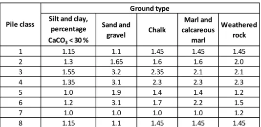
1 ; ; * * (Eq. 2.10)               _ _   B D c e p L B p e e B D b a k k ₀ 1 ; (Eq. 2.11) L B k L B k k L B p L B p L B p           0 ; 1 ; ; 1 (Eq. 2.12)

(35)

Table 2.3 Table for factor kp for bearing capacity of shallow foundations

translated from NF P94-261 (2013)

All those formulas are summarized an extended for all values of De/B in form of a

diagram with different curves for different soil types and dimensions of the foundation (Fig. 2.1).

Fig. 2.1 Diagrams for factor kp for bearing capacity of shallow

foundations after NF P94-261 (2013) a b c kp0 Strip footing  Q1 0.2 0.02 1.3 0.8 Square footing  Q2 0.3 0.02 1.5 0.8 Strip footing  Q3 0.3 0.05 2 1 Square footing  Q4 0.22 0.18 5 1 Strip footing  Q5 0.28 0.22 2.8 0.8 Square footing  Q6 0.35 0.31 3 0.8 Strip footing  Q7 0.2 0.2 3 0.8 Square footing  Q8 0.2 0.3 3 0.8

Soil category  curve for variation of factor of bearing capacity

Expression of kp

Clay and silt Sand and gravel

Chalk Marl and altered

(36)

2.1.2.2 Settlement

The method proposed is in particular relevant for single footings (relatively small shallow foundations). It does not concern very large raft foundations, for which the oedometric method is more appropriate and preferred in France (Combarieu 2006).

The expressions for the spherical (Eq. 2.13) and deviatoric (Eq. 2.14) parts correspond to those proposed by Ménard in the 1960’s, q’ being the area load from the structure and σ’v0 the initial effective stress at the level of the foundation base, and B0 a reference

width of 0.6 m.



q



B E s _v _c c c  _      0 ' ' 9 (Eq. 2.13)







 _             0 0 0 ' ' 9 2 B B B q E s _v _d d d (Eq. 2.14)

Ec is equal to the pressuremeter modulus of the first layer under the foundation, and Ed

takes into account the moduli in depth with the weighting according to Fig. A.26 and (Eq. A.35) in Appendix A.4.

The rheological or structural factor α is given for different soil types and for different ranges of the ratio EM/pl (Table 2.4). The factors λc and λd depend strictly on the form

and on the relative dimensions of the foundation (Table 2.5).

Table 2.4 Rheological factor α for different soil types and different ranges of EM/pl translated from NF P94-261 (2013) Peat Type α EM/pl α EM/pl α EM/pl α EM/pl α overconsolidated or very dense  > 16 1 > 14 2/3 > 12 1/2 > 10 1/3 normally consolidated or normally dense 1 9 to 16 2/3 8 to 14 1/2 7 to 12 1/3 6 to 10 1/4 overconsolidated, altered, disturbed of loose 1 7 to 9 1/2 5 to 8 1/2 5 to 7 1/3  