ECONOMIC GROWTH, AN EVOLUTIONARY PROCESS
THAT GIVES RISE TO AN ATTRACTOR
Alain Villemeur1
Abstract
Economic growth is seen here as the outcome of an entrepreneur-driven process of evolution in the context of an economy of competitive markets. In the course of this process the entrepreneurs implement capital and labour factors, one part of them committed to substitution and the other to complementarity with increasing returns.
The theory demonstrates that the conditions of equilibrium of the different markets give rise to an attractor made up of steady states. The growth determinants for these states are employment, investment and technical productivity, with the profit share in income always being equal to 1/3.
The comparison of what is learned with the empirical reality of the main developed economies demonstrates the interest of this view of growth. The attractors of the United States economy for the period 1960–2000 are given special attention.
JEL classification : O30, O40, O57.
Keywords : Attractor; Evolutionary process; Growth model; Market economy; United States.
1
Université Paris Dauphine, Crea , Place du Maréchal de Lattre de Tassigny 75775 Paris Cedex 16, France
[email protected] should like to express my gratitude to Jean-Hervé Lorenzi, professor at the Université Paris Dauphine, for his invaluable advice and assistance with this research.
1. Introduction
This article aims to explain the mechanism of economic growth with the help of a growth model that is assumed to represent it in the context of a free market economy. Growth is considered to be the result of economic development driven by innovation as initially described by Schumpeter (1934, 1939, 1942), then developed by Nelson and Winter (1982) and Gaffard (1997).
Economic development has the characteristics of an evolutionary process with the entrepreneur as the central figure. This evolutionary process is by nature in perpetual disequilibrium. Could it be characterised by an attractor, as Gaffard (1997, p. 62) and Nelson (2005, p. 66) have assumed? To recap, a dynamic system attractor is a set towards which a system irreversibly evolves after a long enough time. Nelson (2005) justified this question in the following manner: “In their analysis of certain economic phenomena, for example technical advance, many economists recognize that frequent or continuing shocks, generated internally as externally, may make it hazardous to assume that the system ever will get to an equilibrium; thus the fixed or moving equilibrium in the theory must be understood as an “attractor” rather than a characteristic of where the system is”. This article also aims to explore this question.
We retain the definition of an evolutionary process given by Schumpeter (1939, p. 86): “The changes in the economic process brought about by innovation, together with all their effects and the response to them by the economic system, we shall designate by the term Economic Evolution.” This process is driven by entrepreneurs who have perceived opportunities for wealth through innovations that have been implemented.
Following the first evolutionary growth model (Nelson and Winter, 1982), we accept that a growth model must also be based on a model of economic evolution2. It strikes us that an evolutionary economic growth model of this kind raises two major problems. The first relates to the substitutable or complementary nature of capital and labour inputs applied by entrepreneurs, given the innovations brought into the new combinations. The second relates to the nature of the evolutionary process and the equilibrium encountered. These two problematics will be the topic of a discussion that will lead to retaining the founding hypotheses of a new model (Section 2).
We will then draw up a new evolutionary model of economic growth (Section 3) in order to form, for a highly simplified free market economy, a representation of the essential mechanisms of evolution at the heart of growth. The conditions of market equilibrium (goods market, financial market, labour market) are detailed in Section 4. We show that these conditions generate the existence of an attractor formed by a set of steady states characterising long-term growth (Section 5). Some striking lessons come to light regarding distribution of income.
The major theoretical lessons are then compared with the stylised facts (Kaldor, 1961, Barro and Sala-i-Martin, 1995) and the historical data on profit share in income are analyzed. The attractors are identified for the economy of the United States (1960-2000) in particular (Section 6). After creating a synthesis of the lessons learned from this contribution to the theory of growth, lines of progress are identified in order to overcome the limits of current modelling (Section 7).
2
2. Founding hypotheses
The evolutionary process is boosted by innovation, of which Schumpeter distinguishes five forms: the introduction of a new good, the introduction of a new method of production, the opening of a new market, the conquest of a new source of raw materials or half-manufactured goods, the carrying out of a new organisation of an industry, e.g., creation of a monopoly position (Schumpeter, 1934).
What impacts do these innovations have on the economic system, particularly goods output and potential equilibrium? Schumpeter (1934, p. 121) offers an initial response by distinguishing, in his own words, “produce more” and “produce differently”. “Produce more” is symbolic of product innovations, while “produce differently” is symbolic of innovations in processes.
We must go further, however, by specifying the links between capital and labour factors that may underlie “produce more” and “produce differently”. What role do substitution, complementarity or increasing returns have? This is the first question we examine.
These innovations are behind the evolutionary process conducted by entrepreneurs, who are driven to make successive decisions regarding investment, production and labour. In these conditions, what kind of evolution and equilibrium are encountered? This is the second question we shall examine.
2.1. Substitution, complementarity, increasing returns?
The first significant growth model in the theory of growth, the neo-classical model established by Solow (1956), is characterised by a production function (with constant returns to scale) whose two input factors, capital and labour, are substitutable. Economic growth then lies in exogenous sources, natural population growth or technical progress; in the absence of continual improvements in technology, the growth of the production per capita dies out. The Solow model, and those derived from it (Mankiw and al., 1992) proved interesting for explaining the conditional convergence of economies (Barro and Sala-i-Martin, 1995). Yet, technological progress notwithstanding, these models only explain a small part of effective growth and provide no satisfactory explanation for economic growth (Helpman, 2004).
Another vision of the connection between capital and labour-that of increasing returns- has been set forth by numerous economists, in particular Young (1928) and Kaldor (1961, 1972).3 Input factors are seen as complementary, with increase in output simultaneously requiring an increase in capital and labour, a complementarity that is based on the principle of increasing returns to scale. Though empirical assessments of the growth phenomenon teach us about the primarily complementary nature of input factors (Gaffard, 1997),4 increasing returns are not sufficient to provide a subtle explanation for evolutions in the fundamentals of economies, as Salter notably demonstrates (1960).
The work of Romer (1986) and Lucas (1988) brought about a third vision: endogenous growth models. These are generally based on the existence of increasing (or constant) returns as well as a broader concept of capital that encompasses human capital. All these models are a considerable contribution; we can in particular cite the model proposed by Aghion and Howitt (1988), which shows that innovation and capital accumulation can be two essential factors of
3
Young and Kaldor consider that Adam Smith was behind the first observation of increasing returns, due to his considerations on the effects of the division of labour (An Inquiry into the Nature and Causes of the Wealth of Nations).
4
long-run growth. As Barro (1997) then notes, endogenous growth models are important for gaining a better understanding of the continuation of per capital GDP growth in developed economies.
There have, however, been three major criticisms of the theory of endogenous growth. The first, made by Jones (1995), concerns the apparent discrepancy with reality in OECD countries where, since 1950, the number of scientists and engineers working in R&D has tripled in relation to the active population, without creating a corresponding increase in productivity growth.5
The second considers that human capital is not an input like others; this is in keeping with Nelson-Phelps’ approach (1966) whereby education leads to increasing capacity for innovation and adaptation to new technologies. Finally, these models do not succeed in explaining conditional convergence of economies (Aghion and Howitt, 1998).6
Even though this brief account shows that research on the true mechanisms and determinants of growth is still needed, several elements seem well established, in both theoretical and empirical terms. Empirical reality thus encourages us to acknowledge the simultaneous existence of complementary and substitutable inputs in the growth process.
On a theoretical level, some economists, notably Jones and Manuelli (1990) or Howitt (2000), have developed the idea of reconciling increasing (or constant) returns with the convergence of economies linked to the Solow model. They have thus, as Barro and Sala-i-Martin point out, demonstrated the relevance of a production function considered to be the combination of an AK function and a Cobb-Douglas function, without, however, being able to give a justification for it. This dual form was also the subject of Lorenzi and Bourlès’ first works (1995) and led to Villemeur researching and elaborating a new growth model (2002, 2004) in order to help to explain situations of economic divergence.
These various elements of reflection have led us to posit that growth is the result of an evolutionary process during which firms implement new productive combinations spurred by innovation, with capital and labour inputs being in part substitutable and in part complementary with increasing returns to scale.7 Capital8 is thus substituted for labour over vintage capital (“produce differently”), while capital can give rise to increasing returns through the implantation of extra machines (“produce more”) ; substitution and complementarity are the two facets of “creative destruction”.
2.2. Which evolution, which equilibrium?
As Nelson and Winter (1982) highlighted, the evolutionary process is a process of continuing disequilibrium, taking the decisions made by entrepreneurs into consideration.9 Despite these imbalances, economic trajectories have certain regularities, as Kaldor (1960) first formalised. This invites reflection on the nature of the evolutionary process.
Firstly, we consider that the evolutionary process is led by entrepreneurs making decisions, in production, investment and labour, for example, and as such can therefore seize upon or spark off innovations. Hanusch (1988, p. 2) sums up that vision: “the principal economic agent is
5
The model developed by Aghion and Howitt (1998) overcame this criticism.
6
The authors come to the conlusion that these models (the Solow-Swan and AK models), do not constitute the ultimate explanation of the growth process.
7
Nelson and Winter’s growth model (1982) does not take the dual aspect of production factors into account.
8
In accordance with Nelson-Phelps’ approach, it is accepted that human capital is not a production factor; the capital variable K will therefore not encompass human capital.
9
the entrepreneur, who establishes new combinations by introducing new products as well as new production methods”. This vision of the entrepreneur’s role follows Schumpeter’s and cannot be replaced by the vision of an R&D sector that brings innovations (Ebner 2000). We retain the concept proposed by Gaffard (1997, p.88) of a sequential evolutionary process in production, investment and employment defined as “a succession of balances established over elementary (short) periods, when these balances do not constitute an intertemporal balance over a longer period of time.” Entrepreneurs then make decisions in relation to expectations formulated for the ensuing periods.
The sequential method’s specific approach will be at the heart of the new model put into play. This method will be used to model the sequence of decisions made by the entrepreneur to create new combinations; it also enables use of analytical tools that make it transparent.10 We place ourselves in the framework of a free market economy whose competitive functioning is assumed, in the long run, to bring about conditions of equilibrium in the goods market, the financial market and the labour market. For example, the competitive goods market is thus assumed to oblige entrepreneurs to keep to minimum production costs (Schumpeter, 1942, p. 97). We assume that firms hence aim to reduce production costs (per investment unit); profit is then, by essence, “the result of carrying out new combinations” (Schumpeter, 1934, p. 136).
The free market economy should also favour the regularity of growth (Amendola and Gaffard, 1998).11 Moreover, given the innovation dynamic, it is important to consider the existence of a co-evolution (Malerba, 2006) between technique, firms, innovation activities and the different markets.
The attractor is defined as the set of states towards which fundamentals evolve in the absence of disequilibrium. It is determined by simultaneous realization of equilibrium conditions on the different markets: in other words, it is the result of the presumed perfect functioning of the markets.
3. The evolutionary model of economic growth
3.1. The sequential and dual evolutionary process in a free market economy
Generally speaking, we consider that entrepreneurs ensure production of a technique A, using different vintages of machines.12 By installing additional production machines, they make complementary use of capital and labour to create extra output.13 By replacing, for an unchanged volume of output, old machines by new, more efficient ones that therefore require fewer staff, they are substituting capital for labour.14
10
The Nelson and Winter model (1982), based on Markovian processes and a simulation, has the drawback of not being analytical.
11
“The viability of the growth process, then and not stability is the relevant concept. This depends mainly on the functioning of prevailing institutions (markets, governments, and so on), that is, on the ability of these institutions to provide the means and the environment that make it possible for the economy to remain viable by continuously adapting to shocks and imbalances as they arise” (p. 6).
12
The idea of the vintage capital model was put forward by Johansen (1959) and was then the subject of numerous studies.
13
These machines can be new or old designs.
14
This hypothesis complies with the by-doing model developed by Arrow (1962). Thanks to learning-by-doing, the machines that are built are increasingly efficient; this is materialised in a reduction in the number of workers needed to operate them.
In “produce more”, capital and labour are complementary, as returns are increasing. Production-employment elasticity will be assumed to be variable, given the extreme diversity of productive combinations that can be retained, calling on different levels of per capita production. In “produce differently”, capital is substituted for labour, with jobs being cut in relation to volumes of investment;15 here too various combinations can be retained.
According to the terminology introduced by Phelps (1963), the technique is assumed to be a putty-putty model, given the perfect substitutability of the inputs, as in the Solow model. Complementarity is employed for new production equipment and the proportion of factors is not fixed, due to the existence of numerous possible technical combinations. For previously installed equipment, the different machine vintages make it possible to substitute capital for labour, again variably depending on the combinations used.
The evolutionary process wherein an entrepreneur implements a new productive combination is sequential, with entrepreneurs being led to make successive investment, production and employment decisions while taking consumer demands into account and formulating expectations for the ensuing periods.16 During this process, remunerations are paid to employees and entrepreneurs (or shareholders). The orientation of productive combinations therefore depends on the price of factors, which places income distribution at the heart of firms’ investment decisions.
Throughout this process, we take it that consumers reinforce these choices; in other words, production-demand balance is achieved throughout the sequence of decisions. For the sake of simplification, we accept that for each period the prices of goods are fixed.17
Given the competition in the goods market framework, entrepreneurs will aim for competitiveness through their investments throughout the sequence. One condition for equilibrium is that entrepreneurs adopt productive combinations that minimise the unit production cost (per investment unit) related to the investments made, while taking into account the return on capital expected18 by the financial market (Robinson, 1954).
In the financial market framework, the condition for equilibrium imposes an expected return on capital equal to return on capital. As Robinson theorised (1954, pp. 130-131), if this condition is not met, the volume of invested capital is not adapted. We also accept that in the long-term, the return on capital is a constant through time, while entrepreneurs aim to keep the profit share in income constant; this amounts to the definition of neutrality for technical progress as per Harrod.19
The condition for equilibrium in the labour market framework is that entrepreneurs aim to implement productive combinations for which wage gains are independent of the employment
15
These latter considerations are coherent with the stylised fact (Pianta, 2006) which states that product innovation contributes to creating jobs, while process innovation contributes to cutting jobs.
16
A simple model of the investment and output sequences (Nelson and Winter, 1982) that corresponds to Schumpeter’s analysis is Yit = A it K it , the output Yit of a firm i at time t being equal to capital stock times the
technical productivity it is employing (p.284). Note that this function is similar to the AK function proposed by Rebelo (1991).
17
This follows the concept of “temporary equilibrium” defined by Hicks (1939).
18
Return on capital is defined as the ratio between the amount of profit and the volume of capital employed. It is sometimes termed “rate of return on capital”. The return expected by the entrepreneur is assumed to be a function of the financial market’s requirements.
19
These final conditions are indeed equivalent to the conditions defining a neutrality for technical progress in the sense in which Harrod sees it (constancy of the profit share in income and of the capital productivity), as long as the prices of production and capital are constant, which they are in this model.
growth rate.20 With this last condition translating the existence of a wage increase norm that imposes itself on all firms, independently of employment growth. If this condition is not met, the employees of firms that create jobs will be favoured or put at a disadvantage.
The evolutionary process of growth in a free market economy is mainly characterised by these major rules. Nevertheless, for reasons of clarity, other rules specifying it are introduced as the model is constructed.
3.2. Production activity
In the considered economy, goods are production goods as much as consumer goods. We place ourselves at the period [t, t+dt] of a sequence of decisions for an entrepreneur engaged in a process of sequential evolution.
This entrepreneur invests the volume K& to plan for additional output, K being the volume of capital. So x is the share of the increment of capital engaged in “produce more”; x will be named “complementarity rate” in the series. The increment of capital engaged in “produce more” is x &K(x∈R 0≤ x≤1).
The output growth rate
We accept that additional production, linked to a new productive combination using the technique A, takes the form Ax &K.21 The parameter A characterises the productivity of the investment employed in complementarity: it will be termed “technical productivity”22. This parameter is supposed constant over a long period and common to all entrepreneurs. Since, by definition, substitution occurs in continuous production, additional production is written:
K Ax
Y& = & A>0 0≤ x≤1 (1) We assume that production meets demand and that the balance between investment and saving is achieved. Hence:
Axs Axi Y K Ax Y Y = = = & & with K& =I i s Y I = = Y =C+I (2) where I is investment (net), C is consumption, i is investment rate (net) and s is saving rate. These two latter rates are assumed equal and will from now on be called “rate of accumulation”.
The output growth rate is proportional to technical productivity, the complementarity rate and the rate of accumulation. Thus we obtain a simple result: economic growth is self-maintained and all the stronger when the rate of accumulation or the proportion of investment employed in complementarity are high.
The employment growth rate
Let us now address the relation between employment L and investment. In the framework of complementarity, let us designate as the creations of jobs associated to the investment . Accounting for innovations, we accept that the marginal rate of labour productivity
c L K x &
20
In his study of 27 industrial sectors of the American economy from 1923 to 1950, Salter (1960) noted the lack of correlation between labour productivity gains and employment growth. Other economists have also demonstrated this fact in the United States in a similar form: there is no correlation between labour productivity and employment; let us mention the works of Hansen and Wright (1992).
21
It comes, by differentiation in relation to time, from the form proposed by Nelson and Winter (1982) to represent Schumpeter’s analysis.
22
( ) is higher than the labour productivity, the coefficient of proportionality being the elasticity that we will suppose is variable. Returns to scale are increasing and translated by a coefficient higher than the unit, i.e.
c L Y /& c e L Y e L Y c c = & ec >1 ⇒ xs xs e A L L c c c = =ε with c c e A = ε 0<εc < A (3)
where εc is defined as the “job creations coefficient”.
In the substitution framework, the rate of job losses (relation between job losses and employment L) is assumed to be proportional to the rate of investment employed in substitution , with the coefficient of proportionality
l
L
(
1−x)
i εl being named “job losscoefficient”23 i.e ;
(
x)
s L L l l =ε 1− ≥0 l ε (4)Hence the employment growth rate that is the result of the balance between the job creations rate and the job loss rate:
(
x)
s xs L L l c − − =ε ε 1 & εc >0 εl ≥0 A> (5) εc We assume that there is a connection between choices made with regard to complementarity and substitution; when the entrepreneur favours the choice of combinations that tend to create jobs (a higher job creations coefficient), the combinations chosen for substitution destroy fewer jobs (lower job loss coefficient). Consequentially, we set down the following relation:(6) mx c l c ε ε ε + = mx c c ε ε ≤ < 0 0≤εl <εcmx
where εcmx is the maximal coefficient of job creations.24 The constraints of labour organisation impose limits to creating or cutting of jobs. This last parameter reflects the organisational limit to creating or cutting jobs, taking into account the organisations which the entrepreneur has implemented in the context of use of technique A.25
In the end, employment growth is finally written:
(
s xs L L c mx c mx c ε ε ε − − = &)
mx (7) c c ε ε ≤ < 0 A>εcmx
Employment growth rate thus depends on the rate of accumulation, the complementarity rate, the job creations coefficient, and a parameter reflecting the organisational limit to creating or cutting jobs.
4. The conditions of equilibrium in the markets
We will now successively determine the states that are the result of equilibrium in the different markets.
23
In a way this reflects the fact that the entrepreneur cuts jobs in proportion to the “deficit” of demand for his products, a deficit represented by the term A(1−x)s. The job creations coefficient and the job loss coefficient are the elasticities of labor to investment (related to complementarity and substitution).
24
It is also the maximal coefficient of job losses.
25
This is coherent with the stylised fact whereby division of labour is limited by the use of technique and not by the size of the market (Malerba, 2006).
4.1. Taking the goods market into account
We are still considering an entrepreneur at a time t engaged in a sequential and dual evolutionary process in a free market economy. For an investment K& , the entrepreneur must arbitrate between numerous productive combinations. Given the competition, entrepreneurs will aim to minimise the cost of production (per investment unit) that results from the investment; he takes this decision by taking into account return on capital expectations and assuming that wage w is constant.
a
z
The cost of production induced by the investment decision includes the cost linked to employment growth and the cost of invested capital linked to the entrepreneur’s profitability expectations. In the end, the cost of production (per investment unit) is written:
m C m a
[
(
)
cmx(
)
c(
)
cmx a]
z c c x c K K z L w K C + − − − + − = + = 1 ε 1 ε 1 ε . & & & & (8)c being the profit share in income such as wL= 1
(
−c)
Y .In a context of limited rationality, the entrepreneur is supposed to minimise the cost per investment unit under two particular constraints:
- the share of profit c in income is constant in order to maintain the share of profit when choosing new combinations;
- the cost of job creations for output, per investment unit, is inversely proportional to the expected return on capital. This constraint reflects the fact that the greater the expected return on capital, the fewer jobs will be created, given the risks taken by the entrepreneurs who create jobs to produce goods.
Hence the two constraints: 1 c c=
(
)
a c c c z c x c K xs wL K wL 2 1− = = = ε ε & & za ≠0 x ≠0In fact, the entrepreneur’s optimisation programme is the following: at each time t, the entrepreneur’s decisions are deduced from:
⎭ ⎬ ⎫ ⎩ ⎨ ⎧ K C Min m
& , subject to:26 c= c1 xεcza =c'2 The minimisation programme is equivalent to:
(
)
(
)
{
c a}
mx
c x c z
c
Min 1− 1 ε + 1− 1 ε + subject to: c'2=xεcza
To solve this easily, we obtain a function with 2 variables (by substitution of the constraint in the function to be minimised) for which we write the first-order conditions to find the extrema, i.e. c c mx c a c x c c x c z x f ε ε ε ε 2 1 1 ' ) 1 ( ) 1 ( ) , , ( = − + − + 0 ' ) 1 ( 22 1 − = − = ∂ ∂ c mx c x c c x f ε ε (1 ) '22 0 1 − = − = ∂ ∂ c c x c c f ε ε
These conditions define a minimum,27 for it is easy to show that the Hessian matrix of order 2 is defined positive.28 In the end, the conditions of minimisation are written:29
26
In other words, the constraints are exogenous variables at x ,ε ,c za. 27
(
)
mx c a c z x ε − = 1 c z x a mx c c = = − 1 ε ε (9)At optimum competitiveness, the complementarity rate and the coefficient of job creation depend on the expected return on capital. This reflects the fact that the choice of productive combinations is oriented by the expected return on capital. The condition for a solution to exist in the realm of definition requires expected return on capital to be below a level that depends on the technique employed and the share of profits in income.
(
x,εc)
∈] ]
0,1 x]
0,εcmx]
⇔(
)
mx] ]
a(
)
cmx c a z c c z ε ε ∈ ⇔ ≤ − − 0,1 1 1 (10)In the framework of a sequential and dual evolutionary process, the entrepreneur’s competitive choices thus determine, in relation to the expected return on capital for the ensuing periods, the share x of capital engaged in complementarity and the coefficient of job creation εc. Given the relations (7) and (9) :
(
)
s xs L L c mx c mx c ε ε ε − − = & εc =εcmxx⇒ 2 1 2 1 + = L L s x mx c & ε (11)The output growth rate (2) becomes: s A L L A Y Y mx c 2 2 + = & & ε (12)
4.2. Taking the financial market into account
Up to now, return on capital expectations has been formulated throughout the sequential evolutionary process. In conditions of financial market equilibrium, expected return on capital meet return on capital to reach a value at equilibrium which is a time constant, and entrepreneurs keep the profit share in income constant:
e z , constant = = = e a z z z c=constant with K Y c z = (13) This is translated by the following conditions:
e a z z z = = ⇒
(
)
mx c e c z x ε − = 1 K = Y constant⇒ Ac z x c z s Axs K K Y Y& = & = = e ⇒ = e (14)These conditions lead us to determine profit share in income and the complementarity rate:
A c mx c mx c + = ε ε Ac z x= e (15)
4.3. Taking the labour market into account
From now on we take it that the entrepreneur takes the existence of the labour market into account. The condition for equilibrium in this market is defined by a wage increase norm that is imposed on all firms, regardless of the employment growth rate. Given that entrepreneurs maintain a constant profit share in income (financial market), these two conditions are written:
constant = c ⇔ L L Y Y w
w& = & − &
w w& independent of L L&
28
The two principal minor diagonals of the Hessian matrix are strictly positive.
29
The result of the relation (12): s A L L A L L Y Y w w mx c 2 1 2 ⎟⎟⎠ + ⎞ ⎜⎜ ⎝ ⎛ − = −
= & & & & ε ⇒ 2 A mx c = ε (16)
The condition of equilibrium in the labour market forces the entrepreneur to implement productive combinations where the maximal coefficient of job creations is equal to half of technical productivity.
Having taken the labour market into account we have now finished construction of the evolutionary growth model. Table 1 synthesises the relations between the fundamentals and the parameters of this model.
Output growth rate
Axs Y
Y =& A>0 0≤ x≤1 Employment growth rate
(
)
s xs L L c mx c mx c ε ε ε − − = & 0<εc ≤εcmx mx c A>ε Goods market ⎭ ⎬ ⎫ ⎩ ⎨ ⎧ K C Min m& with Cm =wL& +zaK&
subject to: c=c1 xεcza =c'2
Financial market za =z =ze =constant c=constant
Labour market w w& independent of L L& Y : volume of production K : volume of capital L : volume of employment A : technical productivity x : complementarity rate s : saving rate w : wage c
ε : job creations coefficient
mx c
ε : maximal coefficient of job creations
c : share of profit in income
a
z : expected return on capital
z : return on capital
e
z : return on capital at equilibrium
Table 1. Synthesis of the evolutionary growth model.
5. The determination for the attractor
We will now determine the attractor, i.e the states induced by concomitant conditions of equilibrium in the goods market, the financial market and the labour market.
5.1. The existence of steady states of the attractor
From now on we consider an economy where entrepreneurs are engaged in a sequential and dual evolutionary process and equilibrium conditions in the different markets are met. The conditions of equilibrium (12), (15) and (16) provide the following particular results:
3 1 = c ze A x= 3 As L L Y Y 2 + = & & (17) A first striking result comes to light: the distribution of income is 1/3 for capital income and 2/3 for labour income. In other words, the profit share in income is a remarkable constant no matter what the technical productivity, output growth rate or the rate of accumulation.
The second striking result lies in determining the complementarity rate in relation to return on capital at equilibrium. As the complementarity rate is constant in time, the output,
employment and wage growth rates are constant in time. Conditions for market equilibrium therefore determine the steady states30 of growth that depend only on return on capital at equilibrium.
The third striking result lies in the fundamental relation of production verified by the attractor: s A L L Y Y 2 + = & & (18) What then are the determinants of growth? The output growth rate is simply the sum of the employment growth rate and half of technical productivity times the rate of accumulation. The determinants of growth are therefore the employment growth rate, the rate of accumulation, and technical productivity.
Fundamentals Expressions Comments
Output growth rate
Axs K K Y Y = = & &
Employment growth rate
(
)
s x A L L 2 1 2 − = &
Fundamental relation of production
s A L L Y Y 2 + = & &
Growth rate of labour productivity and of total productivity s A w w PL 2 = = & PT As 3
= PLis equal to the wage growth rate.PT is equal to 2/3 of PL. Profit share in income
3 1 =
c The share of the labour in income is 2/3
Return on capital and
productivity of capital ze Ax
3
= Ax K
Y = The complementarity rate is a function of ze, with
3
A ze ≤ Table 2. Expression of the fundamentals in the attractor.
Table 2 sums up the expression of the main fundamentals in the attractor. In the end, they are all expressed in relation to parameter A of technical productivity and the exogenous variables of the rate of accumulation (s) and equilibrium return to capital (ze).
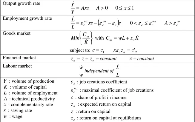
To illustrate this, let us consider a constant rate of accumulation. Graphically (Figure 1), the operating zone over the period [t, t+dt] of an economy confined to one entrepreneur is thus a diamond (excluding ) that extends depending on the rate of accumulation. The line segment represents the case of a maximal coefficient of job creations .
mx A A0 0 mx OA mx c c ε ε =
All the conceivable states of growth are inscribed in the diamond in Figure 1. The attractor is represented by the line segment in Fig. 1 (excluding ); the slope of this line segment is simply equal to the unit. The steady state associated to the expected return on capital is point A. O A A A mx mx 0 0 mx A A0 A0 e z mx
A is the symbol of a growth path of complementarity, with all the productive combinations engaged in complementarity; the production and employment growth rates are then maxima.
30
« The steady state is a convenient analytical device for modeling the long run for -distinguishing between effects that last and effects that are transient » (Aghion and Howitt, 1998, p. 9).
Y Y • mx A0 0 A L L •
Figure 1. The attractor of the economy.
mx A O 2 / As − m A As 2 / As s ze 3 A Mixed growth Complementarity growth
5.2. Limits of growth paths
Another striking result lies in the existence of a return on capital that increases with the complementarity rate. This tends to incite entrepreneurs to invest a growing share of capital in complementarity, which leads to the expected rise in return on capital. This obviously stems from the existence of increasing returns. As a result, the economy heads towards rapid growth until it meets constraints, e.g., in the labour market.
Could other incentives exist? It is interesting to examine the entrepreneur who aims for cost equilibrium for substitution. For such growth paths we would then have:
(
)
(
)
(
)
(
)
(
)
2 1 3 1 2 1 1 1 = ⇔ = − = − − − ⇔ = − x Ax w s x LA K s x L K x z w L K x c mx c l & & & ε ε (19)So for a complementarity rate of 0.5, the productive combinations are at cost equilibrium for substitution. The equivalent growth path (named “mixed growth”) is the point in Figure 1,
with employment growth then being zero; symbolises the mixed productive
combinations. Below this complementarity rate lies an incentive to invest in the substitution of capital for labour, since the reduction of labour costs is higher than the cost of capital invested.
m A m
A
It has so far been implicitly assumed that the economy was in a situation where the capacity utilisation ratio (CUR) was constant. Let us now put ourselves in the case where the CUR
( ) is rising or falling while the complementarity rate still lies between 0 and 1. We assume
that job creations and cuts linked to the evolution of the CUR occur while keeping labour productivity constant. Given the growth rate of the CUR, the relations of production and employment become: c U c c U U Axs Y Y& & + =
(
)
c c c mx c mx c U U s xs L L& & + − − =ε ε ε (20)Depending on the evolution of the CUR, strong economic growth higher than complementarity growth can be obtained, as can recession; these extreme cases can be interpreted as situations where the equivalent complementarity rate would be higher than 1 or negative. The same conditions (9) are obtained in the goods market, with the growth rate of the CUR being assumed exogenous. The same condition (16) is also obtained in the labour
market. Consequentially, the same fundamental relation of production (18) is always verified when the CUR is rising or falling.31 In other words, the line carrying the segment
continues to act as an attractor.
mx
A A0
5.3. The major theoretical result
Economic growth has been considered as the result of economic development stimulated by innovation and driven by entrepreneurs. Economic development has been modelled as a sequential and dual evolutionary process during which entrepreneurs implement a combination of “produce more” and “produce differently”. The sequential method has turned out to be very useful for modelling investment, production and employment choices in relation to return on capital expectations.
It has been demonstrated that the equilibrium conditions that characterise the goods market, the financial market and the labour market bring about an attractor formed by steady states -with growth rates in production, employment and wage remaining constant in time- in the hypothesis that technical productivity and the rate of accumulation are constant. The attractor verify the following fundamental relation of production:
s A L L Y Y 2 + = & & (21) The result is that the determinants of growth are the employment growth, the rate of accumulation and technical productivity (marginal). The greater the share of investments in complementarity, the stronger the growth and the return on capital too. In other words, the more entrepreneurs manage to be engaged in increasing returns, the more growth and return on capital will increase.
How can we interpret the continuing disequilibrium and the attractor? Generally speaking, growth paths appear in disequilibrium, competitiveness is thus not ensured since entrepreneurs do not adhere to the least unit cost of production. One reason for these unsuitable choices springs classically from dependency on the technological trajectory, as numerous economists have shown.32 Given the competition, these entrepreneurs are ultimately obliged to formulate adaptive expectations, i.e., adopt more competitive productive combinations or else disappear. For these entrepreneurs, a return to the optimal situation, steady states between the two limit growth paths, is thus imperative; nonetheless, other entrepreneurs risk being uncompetitive in the ensuing periods.
Economic trajectories, in continuing disequilibrium, will therefore perpetually draw close to and away from attractor, in other words from line segment . The attractor symbolises states of economic evolution when market functioning is presumed perfect. Economic trajectories will be influenced by the attractor, with the restoring force being generated, in a way, by the competitive operation of the markets. Which thus prevent the disequilibrium from degenerating into extreme situations. In the long run, the attractor should also be characteristic of long-term growth, given the properties of steady states.
mx
A A0
6. Confrontation with empirical reality
These major theoretical results will be compared with the reality of the main developed economies since the 19th century. They are relative to the theoretical evolutions of the
31
Note that the conditions stemming from the financial market differ: when the CUR progresses, the states are no longer steady states.
32
fundamentals of the attractor, which will be compared with stylised facts, the empirical distribution of income and the determinants of growth in the United States.
6.1. Stylised facts
By analysing the fundamentals of the main 19th and 20th century economies, Kaldor (1961) identified six stylised facts that characterise long-term economic growth.33 For Barro and Sala-i-Martin (1995), these facts are confirmed by the most recent long-term data from today’s developed countries.34
Fact 1: “Per capita output grows over time, and its growth rate does not tend to diminish”. This is the case in all steady states of the attractor for the per capita output growth rate is constant in time and equal to half of technical productivity times the rate of accumulation. Remember that technical productivity has been assumed constant in the long-term and that economic data shows that rates of investment can be relatively constant over long periods (see below).
Fact 2: “Physical capital per worker grows over time”. This is the case in all steady states. This fact is the result of fact 1 and of the hypothesis on the constancy of the productivity of capital.35
Fact 3: “The rate of return to capital is nearly constant”.36 This is the case, by hypothesis, of equilibrium conditions in the financial market.
Fact 4: “The ratio of physical capital to output is nearly constant”. This fact is the result of the hypothesis already made for fact 2.
Fact 5: “The shares of labour and physical capital in national income are nearly constant”.37 This fact is the case, by hypothesis, of equilibrium conditions in the financial market.
Fact 6: “The growth rate of output per worker differs substantially across countries”. The model teaches that the growth rate of productivity of labour is a function of technical productivity and the rate of accumulation. Consequently, the model anticipates that these growth rates as variable given that these parameters differ from country to country.
Barro and Sala-i-Martin (1995) brought out other stylised facts:
The relative constancy of the rate of accumulation over a long period: in the model, the accumulation rate is assumed to be constant.
The positive correlation between the economic growth and the investment rate:38 for the attractor, the output growth rate is a linear function of the accumulation rate.
The hypotheses or teachings of the model thus prove to be coherent with stylised facts.
33
We follow the presentation and formulation given by Barro and Sala-i-Martin (1995, p.5).
34
Only Fact n° 3 seems questionable, according to Barro and Sala-i-Martin.
35
This is due to the conditions of equilibrium in the financial market.
36
For Barro and Sala-i-Martin, this stylised fact does not seem to be systematically verified, if one considers real interest rates as indicators. Like other economists (e.g. Schubert, 1996, or Hairault, 2004), here we have retained the definition initially given (the return on capital) by Kaldor.
37
The long-term constancy of the distribution of income was a matter of debate among economists well before Kaldor gave it the status of stylised fact. Keynes (1939) invoked “Bowley’s Law” on this subject.
38
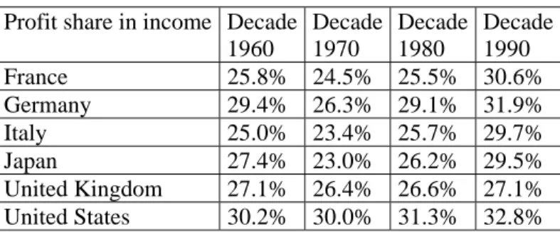
6.2. The distribution of income
In Cobb-Douglas’ first growth model (1928), profit share in income is a constant parameter, evaluated at 30%. Empirical studies confirm this level of percentage for industrial economies, but this was nonetheless susceptible to broad variations in the 19th century (Grangeas, 1991). Let us cite the evaluation for France from 1820 to 1913, with a share that could evolve to the order of 35% with 10 point variations (Levy-Leboyer and Bourguignon, 1985), the evaluation for Great Britain from 1924-1950 with a share of around 35% (Salter, 1960) and the evaluation for the United States in 1909-1949, with an average 34% share (Solow, 1957).39 A 34 % share of profit also characterises as average a set of economies in around 1990 (Gollin, 2002).40
The share of income between profit and wage has been well measured since the 1960s (European Commission, 2001). Particularly the wage share is calculated for the whole of the economy, with the remainder reflecting the profit share in income. Table 3 gives the profit share in income for the six main developed economies.
Profit share in income Decade 1960 Decade 1970 Decade 1980 Decade 1990 France 25.8% 24.5% 25.5% 30.6% Germany 29.4% 26.3% 29.1% 31.9% Italy 25.0% 23.4% 25.7% 29.7% Japan 27.4% 23.0% 26.2% 29.5% United Kingdom 27.1% 26.4% 26.6% 27.1% United States 30.2% 30.0% 31.3% 32.8%
Table 3. Evolution of the profit share in income.
The largest developed economy, the United States, always has a profit share in income between 30% and 33%, which is very close to the theoretical value of 33%. Moreover, growth in this economy is very steady for this period, always between 3.2% and 4.2%.41 America’s performances confirm the existence of a distribution of revenue of the order of 30% to 33% in favour of profit; this is compatible with strong long-term growth, as the evolutionary growth model holds.
The other developed economies do not possess these properties for the period 1961-2000. Their economic growth drops sharply during the 1970s in the wake of the oil crisis in 1973, while profit share in income decreases during this decade before then rising again. In all countries income distribution returns to the original level, however, with a larger share for profit at the end; only the United Kingdom proves to be an exception to this rule. Furthermore, all these economies were profoundly impacted and transformed by the arrival of information and communication technologies (ICT) from the 1980s. In initial analysis, this technological advent did not strongly impact income distribution in the long run.
The historical data thus amply confirms the theoretical existence of constant distribution of income, 1/3 for profit, 2/3 for wage. This distribution also seems to be insensitive to economic or technological shocks in the long term, as illustrated by the economy of the United States.
39
Annually, the share evolves between 31% and 40%.
40
This average characterises a set of 41 economies, the share of profit evolving from 20% to 35%.
41
6.3. The determinants of growth and the attractors in the United States
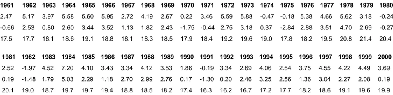
Theory shows that output growth rate (for the attractor) is a linear function of employment growth rate and the rate of accumulation, with the coefficient of employment being equal to 1 and the coefficient of accumulation half of technical productivity. We will verify whether a correlation such as this exists for the largest developed economy, the United States, between annual GDP growth rates on the one hand and, on the other, annual employment growth rate and rate of investment taken as a measure of the rate of accumulation. The chosen period is 1960-2000, a period for which precise annual data on GDP growth, employment growth (in hours worked),42 and rate of investment is available (data in Appendix).
Our choice of the American economy is justified by the existence of two highly interesting properties in relation to the theory: strong steady average growth and quasi constancy in the share of profit throughout the period (see Table 3). It should be noted that the American economy is the only one to display these characteristics over the period in question; the other economies experienced strong economic slowdown and major variations in income distribution, as we saw earlier.
The fundamental relation of production
Let us start by examining the correlations between production and employment. We will also single out two very different sub-periods, the 1960-1973 period before the oil crisis of 1973, and the 1980-2000 period (after the oil crisis of 1979), which is characterised by two long growth cycles and the rapid emergence of ICT.43 Significant straight linear regressions are obtained:44 1960-2000 1960-1973 1980-2000 0188 , 0 94 , 0 + = L L Y Y& & (0.10) (0.0025) 0266 , 0 89 , 0 + = L L Y Y& & (0.15) (0.0036) 0169 , 0 95 , 0 + = L L Y Y& & (0.16) (0.0036)
In accordance with the theory, the coefficient of employment is very close to 1. It is interesting to note that in their study of the evolution of production and employment in ten industries in the years 1924-1939 and 1955-1988, Bernanke and Parkinson (1991) demonstrated an average coefficient of employment in the linear regressions of 1.07 and 0.96 respectively.45 Furthermore, these results seem robust, for they are not very sensitive to the annual limits chosen; considering the periods 1979-2000 or 1974-2000, for example, would have led to very similar results.46
42
The data comes from the World Bank (WDI) for GDP growth rate and for rate of investment and from the Groningen Centre database for the growth rate of the total hours worked. Since the database lacks a net rate of investment, we have assumed that the proportion of investments for replacement is classically 30%.
43
The growth cycles are from 1983 to 1990, then from 1991 to 2000.
44
The values in brackets are the standard errors linked to the coefficients. The R2 are 0.68, 0.75, and 0.68 respectively. The t statistics for the three respective periods are 9.00 and 7.48, then 5.75 and 7.42, then finally 6.15 and 4.72.
45
In 72% of cases, the coefficients for the different sectors are between 0.8 and 1.3. They are obtained from quarterly observations for each of the ten industries. It should be noted that the first period, 1924-1939, which covers the years of the Great Depression, confirms this property of the coefficients while extreme economic disruptions were in play.
46
The coefficient of employment (and the constant term) would have been 1.01 (0.0151) and 0.96 (0.0152) for 1979-2000 and 1974-2000 respectively, with R2s of 0.70 and 0.72.
The result of the coefficient in relation to very long-term investment is that technical productivity is 0.29.47 Another method for determining this technical productivity stems from the fundamental relation of production by considering the average values of the fundamentals for the period 1960-2000;48 the value we obtain is 0.27, which tallies with the value obtained from the linear regression.
Basing itself on the evaluation of technical productivity, the theory can predict a 8.7% return on capital.49 This prediction appears satisfactory, since return on capital is estimated in the region of 10% over this period (Romer, 1996)50. The evaluation of technical productivity thus seems coherent with the fundamental of return on capital.
The role of the fundamental relation of production as an attractor
The good agreement between the technical productivities obtained by linear regression and average values confirms the part which fundamental relation of production plays as an attractor.
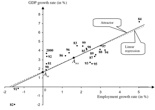
As an illustration, Figure 2 represents the fundamental relations of production for the period 1980-2000 obtained theoretically (attractor)-from the average annual values over the period-and empirically, by linear regression.
Figure 2 also illustrates the imbalanced nature of annual economic growth and the role the fundamental relation of production plays as an attractor. The annual economic growth trajectory curls around the attractor, with the long-term average values of the fundamentals being coherent with those of the attractor.
GDP growth rate (in %)
Figure 2. The attractor for United States (1980-2000)
Employment growth rate (in %) m A 82 91 2000 92 81 90 86 96 83 99 98 85 93 95 87 89 88 94 97 84 mx A Attractor Linear regression 8 7 6 5 4 3 2 1 -2 -1 -2 -1 0 1 2 3 4 5
47
The average rate of investment (net) is 0.131.
48
The average GDP growth rate is 3.41%, the average employment growth rate is 1.64% (and the average rate of investment (net) is 0.131).
49
It is calculated from the evaluation of technical productivity at 0.29 and the complementarity rate of 0.90 (formula 2) and the average data on the American economy over the period 1960-2000 (see previous note).
50
7. Conclusions
Even though the economy and the evolutionary process have been given a very simplified representation, confronting the growth model with the empirical reality of developed industrial economies confirms how useful this model is for understanding the mechanisms of economic growth. It seems promising to consider economic growth as the result of an evolutionary process in a free market economy-following on from Schumpeter (1934) and Nelson and Winter (1982)-with this process being sequential as Gaffard theorised (1997). Through the theoretical and empirical considerations we have developed, economic growth proves to be the result of a sequential and dual evolutionary process driven by entrepreneurs. It has been demonstrated that the evolutionary process has an attractor generated by conditions of equilibrium in the goods market, the financial market and the labour market. The attractor, formed by steady states, respects the fundamental relation of production:
s A L L Y Y 2 + = & &
The determinants of long-term growth are thus employment growth, the rate of accumulation, and technical productivity (marginal). Their existence has been empirically demonstrated by studying correlations in the U.S. economy in the period 1960-2000, a period for which the necessary annual data is available and which fulfils the theory’s conditions, i.e., regular growth and relatively constant distribution. The linear regression turned out to agree well with the fundamental relation of production, including during the two sub-periods characteristic of before and after the oil crises.
Economic growth thus appears to be a process in continuing disequilibrium characterised by an attractor (Gaffard, 1997, Nelson, 2005). The paths of growth curl themselves around this attractor, in a way, without ever durably reaching it.
The interpretation is that of a naturally imbalanced evolutionary process in a free market economy, yet whose different markets channel the disequilibrium around the attractor. Let us take the example of the competitive goods market: competitive entrepreneurs are those who minimise production cost (per investment unit). Yet given their technological path dependency, non-competitive entrepreneurs are driven to draw inspiration from the former or else disappear; the learning and selection process thus forces them to return to the attractor while other entrepreneurs in turn run the risk of being non-competitive. In the end, the attractor is the consequence of the existence of different competitive markets. Made up of steady states, this attractor is also characteristic of long-term growth.
The theory proves to be in phase with stylised facts (Kaldor, Barro and Sala-i-Martin). It has also shown a theoretical income distribution of 1/3 for capital income and 2/3 for labour income. That property matches the empirical reality for the United States.
Here we confine ourselves to citing the three limits that strike us as being particularly prejudicial. The first is the fact that R&D efforts and human capital are not considered in the model. We can reasonably assume that these factors play a major part in the evolutionary growth process; empirical results indeed suggest that the most successful steady state is that of the most innovative economies. The second is the hypothesis of constant distribution of income; it seems interesting to develop a growth theory taking an evolving distribution into account. The third lies in the absence of consumer behaviour models; consumer propensity to consume new products and thus favour distribution of innovations is probably a factor that favours strong implementation of increasing returns. These limits deserve to be worked on in order to be surmounted.
References
Aghion, P. and P. Howitt, (1998), Endogenous Growth Theory, MIT Press.
Amendola, M. and J.-L Gaffard, (1998), Out of Equilibrium, Clarendon press, Oxford.
Arrow, K. J. (1962), “The Economic Implications of Learning by Doing”, Review of Economic Studies 29, pp. 155-173.
Barro, R. J. (1997), Determinants of Economic Growth. A Cross-Country-Empirical Study, Massachusetts Institute of Technology.
Barro, R.J. and X. Sala-i-Martin, (1995), Economic Growth, McGraw-Hill, Inc.
Bernanke, B. and M. Parkinson, (1991), “Procyclical Labor Productivity and Competing Theories of the Business Cycle: Some Evidence from Interwar U.S. Manufacturing Industries”, Journal of Political Economy 99 (June), pp. 439-459.
Cobb, C. W.and P. H. Douglas, (1928), “A Theory of Production”, American Economic Review 18, March, pp. 139-165.
European Commission, (2002), European Economy, 2001 Review, n° 73, Brussels.
David, P.A. (2000), “Path Dependance, its critics and the quest for ‘historical economics’”, Economic History, February.
De Long, J.B. and L.H. Summers, (1991), “Equipment Investment and Economic Growth”, Quarterly Journal of Economics, 106, 2 (May), pp. 445-502.
Ebner, A. (2000), “Schumpeterian Theory and the Sources of Economic Development: Endogenous, Evolutionary or Entrepreneurial?”, International Schumpeter Society Conference on “Change Development and Transformation: Transdisciplinary Perspectives on the Innovation Process”, Manchester, 28 June-1 July. Gaffard, J.-L. (1997), Croissance et fluctuations économiques, 2nd edition, Montchrestien.
Gollin, D. (2002), “Getting Income Shares Right”, Journal of Political Economy, vol. 110, n°2, pp.458-474. Grangeas, G. (1991), Croissance cycles longs et répartition, Economica.
Hairault, J-O. (2004), La Croissance, Théories et Régulations empiriques, Economica.
Hansen, G. and R. Wright, (1992), “The Labor Market in Real Business Cycle Theory”, Federal Reserve Bank of Minneapolis, Quaterly Review 16 (spring), pp. 2-12.
Hanusch, H. (1988), Evolutionary Economics, Application of Schumpeter’s ideas, Cambridge University Press. Helpman, E. (2004), The Mystery of Economic Growth, The Belknap Press of Harvard University Press.
Hicks, J.R. (1946), Value and Capital: an inquiry into some fundamental principles of economic theory, second ed. Clarendon Press, Oxford (first ed., 1939).
Howitt, P. (2000), “Endogenous Growth and Cross-Country-Income Differences”, American Economic Review 90, pp. 829-846.
Johansen, L. (1959), “Substitution versus Fixed Production Coefficients in the Theory of Economic Growth: a Synthesis”, Econometrica 27.
Jones, C. I. (1995), “R&D-Based Models of Economic Growth”, Journal of Political Economy 103, pp. 759-784. Jones, L. E and R. E. Manuelli, (1990), “A Convex Model of Equilibrium Growth: Theory and Policy
Implications”, Journal of Political Economy, 98, 5 (October), pp. 1008-1038.
Kaldor, N. (1961), “Capital Accumulation and Economic Growth”, in F.A. Lutz, and D.C. Hague (eds), The Theory of Capital, Macmillan, London. Also in Further Essay on Economic Theory, Duckworth, London, 1978.
Kaldor, N. (1972), “The Irrelevance of Equilibrium Economics”, Economic Journal. Also in Further Essays on Economic Theory, Duckworth, London, 1978.
Keynes, J.M. (1939), “Relative Movements of Real Wages and Output”, Economic Journal, mars, pp. 34-51. Levine, R. and D. Renelt, (1992), “A sensitivity Analysis of Cross-Country Growth Regressions”, American
Economic Review, 82, 4, September, pp. 942-963.
Levy-Leboyer, M. and F. Bourguignon, (1985), L’économie française au XIXe siècle, Economica. Lorenzi, J-H. and J. Bourlès, (1995), Le choc du progrès technique, Economica, January.
Lucas, R.E. (1988), “On the Mechanics of Economic Development”, Journal of Monetary Economics, July, 22, pp. 3-42.
Malerba, F. (2006), “Innovation and the Evolution of Industries”, Journal of Evolutionary Economics, 16, n°1-2, April, pp. 3-23.
Mankiw, N., D. Romer, and D.N. Weil, (1992), “A Contribution to the Empirics of Economic Growth”, Quarterly Journal of Economics 107, pp.407-438.
Nelson, R. and E. Phelps, (1966), “Investment in Humans, Technological Diffusion and Economic Growth”, American Economic Review 61, pp. 69-75.
Nelson, R. and S. Winter, (1982), An Evolutionary Theory of Economic Change, Belknap Press of Harvard University, Cambridge, Mass.
Nelson, R. (2005), Technology, Institutions and Economic Growth, Harvard University Press, Cambridge. Phelps, E. S. (1963), “Substitution, Fixed Proportions, Growth and Distribution”, International Economic
Review, September.
Pianta, M. (2006), “Innovation and Employment”, in J. Fagerberg, D. Mowery, and R. Nelson, (2006), The Oxford Handbook of Innovation, Oxford University Press, pp. 568-598.
Rebelo, S. (1991), “Long-Run Policy Analysis and Long-Run Growth”, Journal of Political Economy, June, 96, pp. 500-521.
Robinson, J. (1954), “The Production Function and the Theory of Capital”, Review of Economic Studies 21. Reprint 1964 in Collected Economic Papers, vol. 2, Basil Blackwell, Oxford, pp. 130-131.
Romer, D. (1996), Advanced Macroeconomics, McGraw-Hill, Inc. French translation: Macroéconomie approfondie, 1997, Collection Sciences Economiques, Ediscience international.
Romer, P. M. (1986), “Increasing Returns and Long-Run Growth”, Journal of Political Economy, October, 94: 5, pp. 1002-1037.
Salter, W. E. G. (1960), Productivity and Technical Change, Cambridge University Press (second ed. 1966). Schubert, K. (1996), Macroéconomie, Comportements et Croissance, Vuibert.
Schumpeter, J. A. (1934), The Theory of Economic Development, Harvard University Press, Cambridge, 1993, Massachusetts (Original edition 1911). Second edition, 1926, French Translation, 1999, Théorie de l’évolution économique, Dalloz.
Schumpeter, J. A. (1939), Business Cycles: A Theorical, Historical and Statistical Analysis of the Capitalist Process. Vol. 1 McGraw-Hill, New-York.
Schumpeter, J. A. (1942), Capitalism, Socialism and Democracy, Harper Torchbooks, 1976, New-York.
Solow, R.M. (1956), “A contribution to the Theory of Economic Growth”, Quarterly Journal for Economics, 70 (February), pp. 65-94.
Solow, R.M. (1957), “Technical Change and the Aggregate Production Function”, Review of Economics and Statistics 39, pp. 312-320.
Verspagen, B. (2006), “Innovation and Economic Growth”, in J. Fagerberg, D. Mowery, and R. Nelson, (2006), The Oxford Handbook of Innovation, Oxford University Press, pp. 487-513.
Villemeur, A. (2002), Nouveau modèle de croissance : une explication des disparités de croissance Etats-Unis- Europe sur la période 1980-2000, Thesis defended on 25 November 2002 at Paris Dauphine University. Villemeur, A. (2004), La divergence économique Etats-Unis – Europe, Economica, January.
Young, A. (1928), “Increasing Returns and Economic Progress”, Economic Journal, December.
Appendix - Data 1961 1962 1963 1964 1965 1966 1967 1968 1969 1970 1971 1972 1973 1974 1975 1976 1977 1978 1979 1980 2.47 5.17 3.97 5.58 5.60 5.95 2.72 4.19 2.67 0.22 3.46 5.59 5.88 -0.47 -0.18 5.38 4.66 5.62 3.18 -0.24 -0.66 2.53 0.80 2.60 3.44 3.52 1.13 1.82 2.43 -1.75 -0.44 2.75 3.18 0.37 -2.84 2.88 3.51 4.70 2.69 -0.27 17.5 17.7 18.1 18.6 19.1 18.8 18.1 18.3 18.5 17.9 18.4 19.2 19.6 19.0 17.8 18.2 19.5 20.8 21.4 20.4 1981 1982 1983 1984 1985 1986 1987 1988 1989 1990 1991 1992 1993 1994 1995 1996 1997 1998 1999 2000 2.52 -1.97 4.52 7.20 4.10 3.43 3.34 4.12 3.53 1.86 -0.19 3.34 2.69 4.06 2.54 3.75 4.55 4.22 4.49 3.69 0.19 -1.48 1.79 5.03 2.29 1.18 2.70 2.99 2.76 0.17 -1.30 0.20 2.46 3.25 2.56 1.36 3.04 2.27 2.08 0.19 20.1 19.0 18.7 19.7 19.7 19.4 18.8 18.5 18.2 17.4 16.3 16.2 16.7 17.2 17.7 18.2 18.6 19.1 19.6 19.9
Table 4. GDP growth rate, employment growth rate and gross rate of investment (in %) of the economy of the United States (1960-2000)51
51The data comes from the World Bank (WDI) for GDP growth rate and for rate of investment. The employment
growth rate (hours worked) comes from the following reference: “The Conference Board and Groningen Growth and Development Centre, Total Economy Database, January 2007, http://www.ggdc.net”.