A case study of low-frequency waves at the magnetopause

HAL Id: hal-00329203

https://hal.archives-ouvertes.fr/hal-00329203

Submitted on 1 Jan 2001

HAL is a multi-disciplinary open access

archive for the deposit and dissemination of

sci-entific research documents, whether they are

pub-lished or not. The documents may come from

teaching and research institutions in France or

abroad, or from public or private research centers.

L’archive ouverte pluridisciplinaire HAL, est

destinée au dépôt et à la diffusion de documents

scientifiques de niveau recherche, publiés ou non,

émanant des établissements d’enseignement et de

recherche français ou étrangers, des laboratoires

publics ou privés.

A case study of low-frequency waves at the

magnetopause

L. Rezeau, F. Sahraoui, E. d’Humières, G. Belmont, T. Chust, N.

Cornilleau-Wehrlin, L. Mellul, Olga Alexandrova, E. Lucek, P. Robert, et al.

To cite this version:

L. Rezeau, F. Sahraoui, E. d’Humières, G. Belmont, T. Chust, et al.. A case study of low-frequency

waves at the magnetopause. Annales Geophysicae, European Geosciences Union, 2001, 19 (10/12),

pp.1463-1470. �10.5194/angeo-19-1463-2001�. �hal-00329203�

Annales Geophysicae (2001) 19: 1463–1470 c European Geophysical Society 2001

Annales

Geophysicae

A case study of low-frequency waves at the magnetopause

L. Rezeau1, F. Sahraoui2, E. d’Humi`eres2, G. Belmont2, T. Chust2, N. Cornilleau-Wehrlin2, L. Mellul2, O. Alexandrova2, E. Lucek3, P. Robert2, P. D´ecr´eau4, P. Canu2, and I. Dandouras5

1_{CETP/UPMC, 10–12 avenue de l’Europe, 78140 V´elizy, France} 2_{CETP/UVSQ, 10–12 avenue de l’Europe, 78140 V´elizy, France}

3_{Space and Atmospheric Group, The Blackett laboratory, Imperial College, Prince Consort Rd, London, UK} 4_{LPCE, 3A avenue de la recherche scientifique, 45071 Orl´eans Cedex 2, France}

5_{CESR, 9 avenue du Colonel Roche, 31028 Toulouse cedex 4, France}

Received: 2 April 2001 – Revised: 10 July 2001 – Accepted: 11 July 2001

Abstract. We present the study of one of the first

magne-topause crossings observed by the four Cluster spacecraft simultaneously, on 10 December 2000. Although the de-lays between the crossings are very short, the features of the boundary appear quite different as seen by the different spacecraft, strongly suggesting the presence of a local curva-ture of the magnetopause at that time. The small-scale fluc-tuations observed by the STAFF search-coil experiment are placed in relation to this context. A preliminary investigation of their behaviour on the boundary and in the neighbourhood magnetosheath is performed in comparison with the theoret-ical model of Belmont and Rezeau (2001), which describes the interaction of waves with the boundary.

Key words. Space plasma physics (transport processes,

dis-continuities, turbulence)

1 Introduction

For many years, scientists have tried to understand the trans-fer of particles through the magnetopause. Various models have been used with this aim in mind with the main diffi-culty arising from the fact that the plasma around the mag-netopause is collisionless and that usual diffusion cannot be invoked. Different experimental studies had given the indi-cation that the small-scale electromagnetic fluctuations are likely to play a significant role in these transfers, by taking the place of the collisions, in particular, the observation of a high level of fluctuations right at the magnetopause. Most of the models, until recently, were based on the assumed existence of local instabilities at the boundary, giving rise to plasma penetration, through either anomalous diffusion or reconnection (tearing instability). Belmont and Rezeau (2001) have recently proposed a different and probably more realistic model for explaining both the origin of the strong magnetopause fluctuations and the mechanism of transfer. Correspondence to: L. Rezeau

(laurence.Rezeau@cetp.ipsl.fr)

These authors suggest that the primary cause lies not in a lo-cal instability, but in the pre-existing magnetosheath fluctua-tions; by studying the propagation of incident magnetosheath waves through the magnetopause, they have shown that these waves convert into Alfv´en waves in the boundary density gra-dient. Moreover, in the presence of a sufficient magnetic field rotation, the resulting Alfv´en waves are shown to be trapped in the boundary, therefore producing a local enhancement of the fluctuation level. The major consequence of this trapped small-scale turbulence is to allow via Hall-MHD effects a micro-reconnection distributed all over the boundary.

The time has now come to confront the model with the Cluster data. Part of the Wave Experiment Consortium (Ped-ersen et al., 1997), namely the STAFF instrument, is de-voted to the measurement of the electromagnetic fluctuations ranging from 0 to 4 kHz (Cornilleau-Wehrlin et al., 1997). The STAFF-SC part of the instrument gives the waveform of the low-frequency range (up to 10 Hz) magnetic fluctua-tions. These data are used primarily in the present analysis, together with data that allow for the large-scale description of the magnetopause: the Flux-Gate Magnetometer (FGM) data (Balogh et al., 1997), the density data from the WHIS-PER instrument (D´ecr´eau et al., 1997), and the particle mea-surements made by CIS (R`eme et al., 1997).

The two magnetopause crossings that are studied here have been chosen only because they were observed during one of the first periods when data were acquired simultane-ously on the four spacecraft. For both crossings, the mag-netic field rotates more than 90◦_{, which is favourable for}

the scenario to be tested. Such large-scale features of the boundary are presented in Sect. 2, using FGM data, in order to replace the electromagnetic fluctuations in their context. Section 3 is devoted to the study of the magnetic fluctua-tions themselves. To investigate the modes observed around the boundary, a minimum variance analysis is performed on the STAFF data. These results are very preliminary, since no other case has been studied yet and no specific multi-spacecraft tool has been used yet for the study.

1464 L. Rezeau et al.: A case study of low-frequency waves at the magnetopause

Table 1. First crossing: Comparison of the directions of the

mag-netopause normal determined by Sibeck’s model, the CP, and the MVA methods, respectively

Angle between CP and model MVA and model CP and MVA S/C

1 23.2◦ 40.2◦ 17.4◦

2 21.5◦ 31.2◦ 12.1◦

3 21.0◦ 43.5◦ 22.7◦

4 19.1◦ 39.9◦ 21.0◦

2 Large-scale behaviour of the magnetopause

On 10 December 2000, the WIND satellite is not in a very good position to place our study in its interplanetary context (GSM: 28.5 RE,185.0 RE,−50.5 RE). However, it indicates

that the pressure of the solar wind and its speed are rather steady around 2 nPa and 700 km s−1_{, respectively. B}

Z

re-verses at just around 8:30, going from 5 nT to 1 nT, ti.e. after the crossings studied here.

Since the magnetopause is, by definition, a magnetic boundary, the identification of the crossings is made first on the magnetic field data. Nevertheless, the previous studies of these regions have shown that the behaviour of the low-frequency waves (ULF-ELF) changes radically at the cross-ing: the level of turbulence is low in the magnetosphere, high in the magnetosheath and even higher right on the magne-topause (Perraut et al., 1979; Anderson et al., 1982; Rezeau et al., 1989); this gives another means of identifying the mag-netopause. On 10 December 2000, the orbit of the spacecraft is outbound and many magnetopause crossings can be iden-tified in quite a short period (Fig. 1), indicating that the mag-netopause is not stationary.

To make a detailed study, we select two successive cross-ings: around 08:15, the spacecraft are in the magnetosheath; they cross the magnetopause around 08:21 to enter the mag-netosphere and then go back to the magnetosheath around 08:25:50. At this time, the spacecraft explore the boundary of the magnetosphere on the evening side, well above the ecliptic plane (XGSE= 0.3 RE, YGSE= 18 RE, ZGSE= 6 RE).

As learned from previous one-spacecraft experiments, mul-tiple boundary crossings can be the signatures of either a global back and forth motion of the magnetopause, or surface wave oscillations on the boundary (see for instance, Aubry et al., 1971). Using the Cluster facility, we should be able to disentangle these interpretations.

To study the large-scale behaviour of the magnetopause, we have used the FGM data with a 4 s resolution, together with the WHISPER data, which give an indication of the variations in the density during the crossings. These data are used first to locate the spacecraft in the different regions; and afterwards to characterize the shape of the magnetopause during both crossings. We assume the limits of the magne-topause are the times when the magnetic field stops rotating. As can be seen in Fig. 2, the two crossings look quite

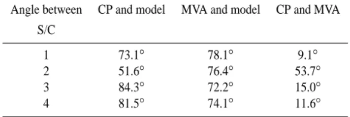
differ-Table 2. Same as differ-Table 1 for the second crossing

Angle between CP and model MVA and model CP and MVA S/C

1 73.1◦ 78.1◦ 9.1◦

2 51.6◦ 76.4◦ 53.7◦

3 84.3◦ 72.2◦ 15.0◦

4 81.5◦ 74.1◦ 11.6◦

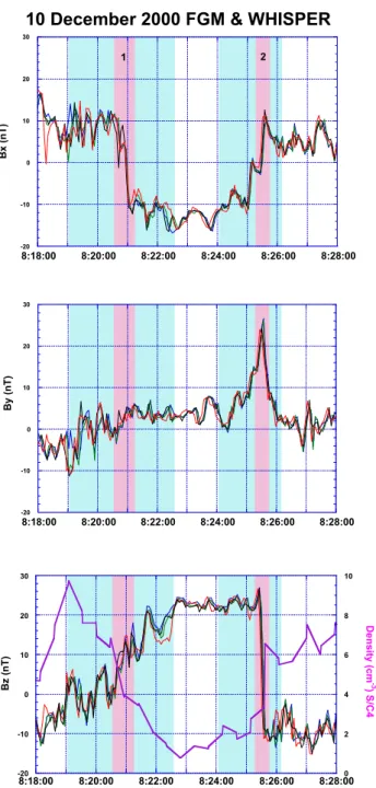
ent, but both seem to be the superposition of two phenomena: a smooth variation of the modulus of the magnetic field and of the density (shown by a blue shading), and sharp rotations (shown by a pink shading). A boundary layer can be seen on the magnetospheric side of the magnetopause in the WHIS-PER data.

Without performing a very detailed study, some informa-tion can be obtained from the variainforma-tions in the magnetic field. We used two different methods to study the magnetopause normal. First, we used the simplest approach, which con-sists of performing the cross product (CP) of the averaged magnetic fields on both sides. Second, we performed a Min-imum Variance Analysis (MVA) (Sonner¨up and Scheible, 1998). Both results are then compared to a model normal using Sibeck’s model (parabolic shape adjusted to the posi-tion where the magnetopause is observed, as calculated by Sibeck et al., 1991), and summarized in Tables 1 and 2.

The CP method is valid whenever one can assume that the boundary is approximately tangential and that the total ro-tation is not too close to 0◦ or 180◦. The comparison be-tween the normals obtained by this method and the normal deduced from the model is presented in the first columns of Tables 1 and 2. One observes that for both crossings, they are always different from each other. During the first crossing, the magnetic field rotates by about 125◦on the four space-craft. The angle between the observed normal and the model one is about 22◦, with the observations on the four spacecraft being similar. Furthermore, the normals of the first crossing are very different from those of the second crossing. During the second crossing, the normals are also different from satel-lite to satelsatel-lite. Three of the CP normals are about 80◦_from

the model normal, while the fourth one is at ≈ 50◦_{. The four}

normals are not in the same plane, which seems to indicate a fully three-dimensional structure of the boundary. Never-theless, these determinations are likely to involve large un-certainties since the rotation angle is not far from 180◦(from 164◦to 172◦, depending on the spacecraft), and a more de-tailed study of this case is therefore necessary.

The MVA method is actually an efficient one as long as the magnetic field variations are polarized in a plane and not along one unique direction; the validity of the result under these conditions is insensitive to the particular case of a 180◦ rotation and gives a more reliable determination of the

mag-L. Rezeau et al.: A case study of low-frequency waves at the magnetopause 1465 10 Figure 1 0 2 4 6 8 10 F re q u e n c y ( H z ) R u m b a (1 ) 0 2 4 6 8 10 12 S a ls a (2 ) 0 2 4 6 8 10 12 S a m b a (3 ) (4) (3) (1) STAFF -SA STAFF -SC (4) (3) (2) (1) 10-4 -10 -6 -2 10 10 10 10 10-6 -4 -8 10 nT /Hz2 2 B2 0 4 8 2 6 10 0 4 8 2 6 10 0 4 8 2 6 10 0 4 8 2 6 10 08:40 08:20 08:00 07:40 (2) nT /Hz 1 B2 B2 10 December 2000 STAFF

Fig. 1. Colour spectrogram of the STAFF data (the horizontal scale is time, the vertical scale is frequency in Hz). The four lowest panels

show the STAFF-SC part, below 10 Hz. The four top panels show the STAFF-SA high frequency band (10 Hz–4 kHz). The thin white line superimposed on the spectrograms is the electron gyro-frequency as deduced from FGM magnetic field. Many magnetopause crossings can be identified: they are identified by arrows on the plot. Red arrows show the two crossings studied in this paper.

netopause normals. The first crossing lasts almost 30 s. We used different time lengths for the minimum variance anal-ysis, ranging from 20 to 110 s. The results are quite stable and are not very different from the previous analysis using only the cross product: we have a mean change of 16◦(see columns 2 and 3 of Table 1). For the second crossing, which lasts for 20 s, we used times ranging from 15 s to 1 or 2 min. The results are also quite stable. As seen in Table 2, the main difference with the cross product analysis concerns space-craft 2, whose normal comes close to the common value of the other spacecraft (about 76◦from the model normal), in-stead of being singular. In the actual conditions of almost 180◦rotations, it is clear that the MVA results are the most reliable, and we will keep them for reference in the follow-ing analyses (Sect. 3). All the precedfollow-ing study tends to show that we are not observing a global back and forth motion of

the magnetopause, but more likely a corrugated surface. The fact that the magnetopause behaves as a surface wave is very important for the study of the small-scale electromagnetic fluctuations on the boundary. As a matter of fact, a previ-ous study performed on ISEE data (Rezeau et al., 1992) has shown that the power of the fluctuations was strongly depen-dent on the large-scale characteristics of the magnetopause, showing (i) that the power of the fluctuations is higher when the boundary is moving earthward and the magnetosphere is compressed, than when it is moving sunward, (ii) when an oscillation is observed on the boundary, the power seemed to be higher on the leading edge of the wave. This study was preliminary and not comprehensive since the measurements were performed with only two spacecraft. Cluster will pro-vide a better view of this problem.

bound-1466 L. Rezeau et al.: A case study of low-frequency waves at the magnetopause 11 -20 -10 0 10 20 30 8:18:00 8:20:00 8:22:00 8:24:00 8:26:00 8:28:00 B y ( nT) -20 -10 0 10 20 30 0 2 4 6 8 10 8:18:00 8:20:00 8:22:00 8:24:00 8:26:00 8:28:00 B z ( nT) Den si ty (cm -3 ) S /C4 -20 -10 0 10 20 30 8:18:00 8:20:00 8:22:00 8:24:00 8:26:00 8:28:00 B x ( nT) 1 2

10 December 2000 FGM & WHISPER

Figure 2 Fig. 2. Three components of the FGM magnetic field projected

in the GSE frame. The time resolution is 4 s. Each spacecraft is identified by the referenced colours (1, black, 2, red, 3, green, 4, blue). In the third panel, an estimate of the density deduced from the WHISPER experiment is superimposed. Blue shading corresponds to the density and magnetic field modulus variations. Pink shading corresponds to magnetic field rotations.

ary can be obtained from the analysis of the delays be-tween the crossings by the different spacecraft. The method that we used for this first estimation is a simple one: for each pair of spacecraft, we assume that the magnetopause is locally a plane moving in the direction of a unique nor-mal n. The velocity of the boundary is determined by

V12 =d12·n/(t2−t1), where d12 is the vector joining the

two spacecraft and t2−t1is the delay between the two

cross-ing signatures. As the tetrahedron is not very large (the maxi-mum distance between spacecraft is 1000 km), the estimation accuracy has to be checked carefully. A reliable value for the delay can be obtained only when the signatures obtained on the two considered spacecraft are sufficiently similar. The parameter that has been used to determine the crossings is the angle between the magnetic field and a fixed direction in the tangential plane. It gives a clear signature of the rotation of the magnetic field. With this parameter, both crossings dis-play a relatively simple structure. For the second crossing, the signatures appear very similar on spacecraft 2 and 4, and fairly similar on spacecraft 1, but spacecraft 3 displays a very different signature, which remains to be explained. Using the spacecraft 2 and 4, a delay of ≈ 4.8 s is observed, leading to a magnetopause velocity of about 230 km s−1_{(along the}

lo-cal normal). For the first crossing, the delays between the spacecraft are shorter (≈ 1 s), and the accuracy of the veloc-ity determination is less reliable. From spacecraft 3 and 4, one obtains nevertheless, a magnetopause velocity of about 154 km s−1.

It is quite interesting to compare the magnetopause veloc-ities obtained in this way with the ion velocveloc-ities measured on board Cluster. Even if the normal component Bn has been

found to be significantly different from zero, which indi-cates that the magnetopause is not strictly tangential and that the magnetosheath and magnetosphere magnetic field lines are “connected”, it is to be expected that the difference be-tween the normal components of these two velocities remains small. We tried to check this with CIS experiment, using CODIF data, which are available on spacecraft 4, and HIA data, which are only available on spacecraft 3. CODIF count rates are partially saturated in the magnetosheath, which re-sults in underestimated velocity values; however, the trends in the velocity direction variations are the same as on HIA. When looking at 3 mn averaged values in the adjacent mag-netosheath or magnetosphere, the ion velocity appears almost tangential to the model magnetopause, independent of the corrugation. When looking at the instantaneous values in the magnetosheath closer to the boundary, the flow appears to turn rather suddenly in the limit of the 4 s resolution, and the velocity along the local normal seems to be close to the ve-locity of the boundary (250 km s−1 on CODIF, 350 km s−1 on HIA). These results are in accordance with the physical guess, but are still preliminary.

The values obtained for the magnetopause velocities of about 150–250 km s−1_{may appear rather high, but it is worth}

noticing that such high values of the normal magnetopause velocity have already been pointed out in the literature using the two spacecraft INTERBALL investigations (Safrankova et al., 1997). All the preceding results intend to place the wave observations in their large-scale context. Figure 3 sum-marizes the main characteristics relevant for this goal. The integrated wave amplitude is placed on a plot where the vari-ations in the Alfv´en velocity are displayed (from CIS and FGM data), as well as the magnetic field rotation angle. The Alfv´en velocity gives a clear signature of the boundary layer

L. Rezeau et al.: A case study of low-frequency waves at the magnetopause 1467 12 -180 -90 0 90 0 0.5 1 1.5 8:20:00 8:21:00 8:22:00 8:23:00 8:24:00 8:25:00 8:26:00

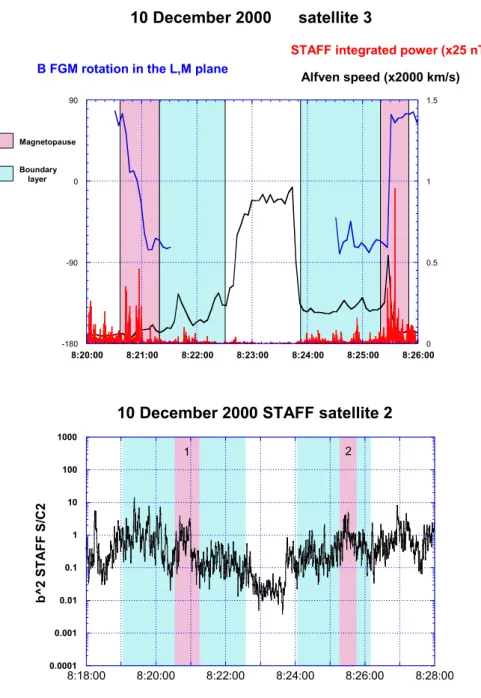
B FGM rotation in the L,M plane

STAFF integrated power (x25 nT2)

Alfven speed (x2000 km/s) Magnetopause Boundary layer

10 December 2000 satellite 3

Figure 3 0.0001 0.001 0.01 0.1 1 10 100 1000 8:18:00 8:20:00 8:22:00 8:24:00 8:26:00 8:28:00 b^ 2 STA FF S /C 2 1 2 Figure 4

10 December 2000 STAFF satellite 2

Fig. 3. Main characteristics of the waves at the magnetopause on space-craft 3: the Alfv´en speed calculated using the density is given by CIS, the magnetic field is given by FGM, the power of the fluctuations from the STAFF experiment (integrated between 0.1 and 10 Hz) are normalised to 1, and the magnetic field rotation angle is the angle between B0and the M direction

in the (L, M) plane. The angle is in-terrupted in the magnetosphere because the (L, M) plane is determined for each crossing and there is no relation be-tween both calculations.

12 -180 -90 0 90 0 0.5 1 1.5 8:20:00 8:21:00 8:22:00 8:23:00 8:24:00 8:25:00 8:26:00

B FGM rotation in the L,M plane

STAFF integrated power (x25 nT2)

Alfven speed (x2000 km/s) Magnetopause Boundary layer

December 10, 2000 satellite 3

Figure 3 0.0001 0.001 0.01 0.1 1 10 100 1000 8:18:00 8:20:00 8:22:00 8:24:00 8:26:00 8:28:00 b^ 2 STA FF S /C 2 1 2 Figure 4

10 December 2000 STAFF satellite 2

Fig. 4. Power of the fluctuations from

the STAFF experiment on spacecraft 2, integrated between 0.1 and 10 Hz.

and shows a local maximum in the second crossing.

3 Small-scale fluctuations

The first information concerning the small-scale variations comes from the distribution of power in the different regions (Fig. 4). As previously observed, the maximum of the power is seen very close to the magnetopause gradient and the level seen in the neighbouring magnetosheath is much lower. The boundary layer corresponds to a level that is comparable to the magnetosheath one. Nevertheless, the contrast between magnetosheath and magnetopause levels appears in this case, weaker than previously reported. Before the first crossing, in particular, when the spacecraft are in the magnetosheath, a very high turbulence is present: it can be seen both at

large-scales on the FGM data and at smaller-large-scales in STAFF data. This observation might be explained by the fact that Cluster crosses the magnetopause on the flanks of the magnetosphere and at a high latitude, which is quite different from previous studies.

The study of the spectra of the fluctuations at the mag-netopause can be expected to yield precious clues for un-derstanding the behaviour of the turbulence near the magne-topause. These spectra are found in this case to follow a f−α power law (Fig. 5), as already observed (Rezeau et al., 1999). A calculation of the parameter α in the magnetosheath and at the magnetopause gives values between 2.3 and 2.9, de-pending on the spacecraft and on the interval studied. These values are consistent with those usually observed except that, contrary to the previous cases, no systematic difference can be evidenced between the slopes at the magnetopause and

1468 L. Rezeau et al.: A case study of low-frequency waves at the magnetopause 13 10-7 10-6 10-5 0.0001 0.001 0.01 0.1 1 1 10 boundary layer (08:25:05:00 ---> 08:25:17:00) magnetopause (08:25:25:00 ---> 08:25:37:00) magnetosheath (08:26:05:00 ---> 08:26:17:00) magnetosphere (08:23:00:00 ---> 08:23:12:00) sensitivity α = −2.82 α = −2.67 α = −2.31 α = −2.88 B² (n T² /Hz) Frequency (Hz)

10 December 2000 STAFF satellite 3

Figure 5

Fig. 5. Comparison of the spectra in the

regions adjacent to the magnetopause on spacecraft 2. For reference, the sensitivity of the instrument is plotted showing that the fluctuations are much higher, even in the magnetosphere.

in the magnetosheath. This may reinforce the observation made on the integrated power: there is less difference be-tween the magnetopause and the adjacent regions observed at high latitudes on the flanks of the magnetosphere than in regions closer to the front of the magnetosphere and at low latitudes.

To test the Belmont and Rezeau (2001) model, it is neces-sary to know how the fluctuations are polarized and whether their polarizations change across the magnetopause. This study has been performed using again a MVA method. The results presented afterward have been obtained for crossing 2, with data filtered in a narrow frequency range (≈ 0.1 Hz) around 0.35 Hz. This frequency is below the proton gyrofrequency in the magnetosphere (≈ 0.4 Hz) and above the magnetosheath one (≈ 0.15 Hz). Under the as-sumption that each data set analyzed is the signature of a plane wave, i.e. with a unique wave vector direction, the MVA technique can indeed provide the main properties of this plane wave: the propagation direction is the direction of minimum variance, and the polarization, linear or elliptic (in the plane perpendicular to propagation), is derived from the maximum and intermediate variances. In the present data, the ratios σ3/σ1of minimum over maximum variances are

found, on average, to be as small as 0.05. The smallness of this ratio evidences the good planarity of the magnetic hodograms that can be drawn as functions of the spacecraft time. In a first step, we used data filtered with a high-pass

fil-ter at 0.35 Hz, but without filfil-tering the high frequencies. The minimum over maximum variance ratios were then about 0.27, indicating that under these conditions, the magnetic variations are not embedded in a plane but in a volume that is still greatly flattened in one direction.

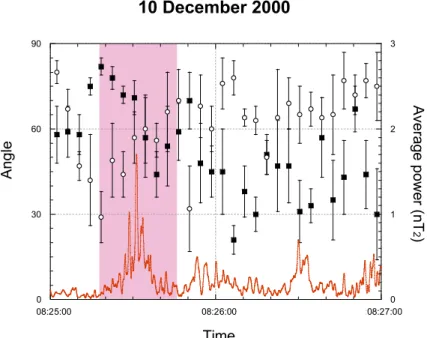
The results obtained in this way have been compared to the main characteristic large-scale directions in the magne-topause vicinity. Figure 6 displays the maximum and mini-mum variance directions as functions of time with respect to the magnetic field direction. To obtain these results, a MVA has been performed on successive 3 s intervals of STAFF data centred around each data point of FGM, i.e. every 4 s. When comparing the mean angles obtained in the magnetosphere and in the magnetosheath, one can see that there exists a sig-nificant trend. The maximum variance is rather perpendic-ular to B0in the magnetosphere (mean value close to 70◦),

indicative of an “Alfv´en type” polarization, while the com-pressional component, parallel to B0, is much larger in the

magnetosheath (mean value close to 40◦). The lowest value lies at the crossing itself where the maximum variance is at only 30◦from B0.

The angle between the minimum variance direction (sup-posedly the wave vector direction) and B0follows an

anti-correlated variation, i.e. rather parallel in the magnetosphere and more perpendicular in the magnetosheath, with a max-imum close to 80◦ at the magnetopause itself. The error bars are generally very large, suggesting that the

polariza-L. Rezeau et al.: A case study of low-frequency waves at the magnetopause 1469 14 0 30 60 90 0 1 2 3 08:25:00 0:08:26:00 0:08:27:00 Time an gl e (° ) av e ra ge po w er (n T₂ ) Figure 6

10 December 2000

Angle Avera ge pow er (n T 2 )

Fig. 6. MVA results for 0.35 Hz

fluc-tuations for crossing 2. The points are the values of the angles between B0and

the direction of maximum variance ( ) and minimum variances (◦) averaged on the four spacecraft. The error bars are the mean square differences of the four values with this average. The position of the magnetopause is shown by the shaded zone and the average power of the fluctuations is drawn for compari-son.

tion directions have a great random component from place to place and therefore, that the waves observed are not pla-nar at the scale of the Cluster tetrahedron. It must be kept in mind that the planarity of the magnetic hodogram as a func-tion of time is not, in general, a proof that we are actually dealing with plane waves. The planarity of the wave sur-faces concerns the spatial and not temporal variations of the magnetic field; a plane hodogram can be considered as an indication of plane waves only when its planarity cannot be attributed to temporal variations that are too simple (in par-ticular, monochromatic). This is probably not the case for the filtered data. This problem will not be solved without using a true 4-spacecraft method, such as multi-spacecraft filtering (Pinc¸on and Lefeuvre, 1998). This work is in progress.

The error bars obtained with the MVA technique are mini-mum close to the magnetopause crossing, rather on the mag-netospheric side of the boundary. The maximum amplitude peak is clearly right in the boundary. The small error bars indicate that at this point one obtains reliable directional in-dicators of the strong waves: a rather parallel propagation, and a shear Alfv´en type polarization. A careful comparison with the model remains to be done.

A comparison has also been performed between the max-imum and minmax-imum variance directions and the magne-topause normal. The main result is that at the point of max-imum amplitude, where the uncertainties are the lowest, the minimum variance direction is almost aligned with the mag-netopause normal. This is in agreement with the fact that the wave vector along the normal direction could increase in this region to values much greater than the tangential compo-nents, as found in the model of Belmont and Rezeau (2001). Outside the magnetopause, no clear trend is observed.

The same work has been done at a frequency around 2 Hz, which is larger than the ion gyrofrequency on both sides of

the magnetopause. The results appear to be rather similar on the magnetospheric side, but a clear trend not longer appears any more in the magnetosheath or at the magnetopause.

4 Conclusion

The results presented here are very preliminary and they need to be confirmed by further studies. They already give a glimpse of the richness of the Cluster data. Looking at a boundary such as the magnetopause with one spacecraft gives a rather simple image. Later on, by using two space-craft missions such as ISEE 1 and 2 (Berchem and Rus-sell, 1982) and INTERBALL-1/MAGION4 (Safrankova et al., 1997) a moving and oscillating layer was detected. Using now the Cluster “microscope” clearly increases the complex-ity of the interpretation. First of all, the large-scale structure of the boundary shows that the layer is not a plane at the scale of the tetrahedron, i.e. some 1000 km, which is very small with respect to the scale of the magnetosphere. It prob-ably cannot be approximated by a two-dimensional surface; rather, it is likely to be fully 3-dimensional locally, which is somewhat far from most models that have described it in the past. From a theoretical point of view, this observation could be related to the Kelvin-Helmholtz instability, whose growth rate is known to maximise for wave numbers of the order of the inverse thickness of the boundary (see, for instance Miura and Pritchett, 1982; Belmont and Chanteur, 1989). For the sake of simplicity, if one visualises the magnetopause as a layer of thickness d limited by two discontinuities, then the theoretical linear results show that: (i) for kd  1, the growth rate increases linearly with k, and the undulations on the two edges are in phase (in this condition, the infinitely thin layer approximation is correct); (ii) for increasing kd, the growth rate increases more slowly where the role of the

1470 L. Rezeau et al.: A case study of low-frequency waves at the magnetopause thickness is to introduce an increasing phase difference

be-tween the two edges; (iii) for kd ≈ 1, the growth rate stops increasing, with the phase difference reaching 180◦_{; (iv) for}

kd > 1, the growth rate falls rapidly down to zero. In con-sequence, as long as the linear fastest growing mode is the most commonly observed, one cannot expect to observe a boundary that would be locally plane. The interpretation of the magnetopause corrugations due to solar wind pressure pulses can lead to similar conclusions.

The wave observations made here confirm the main results obtained by previous experiments. In particular, the observa-tion of a high turbulence level at the magnetopause reinforces the idea that the magnetic fluctuations play a significant role in the physics of this boundary. Nevertheless, most of the previous statistical studies of the turbulence have been per-formed in the front region of the magnetopause. The exam-ple shown here is quite different, since it is an observation of the magnetopause on the flanks of the magnetosphere and at high latitudes. The interaction between the magnetosheath turbulence and the boundary might be different in this region due to, for instance, a large plasma flow. This should be in-vestigated using plasma data in the near future.

As a result of the study performed on ISEE data (Rezeau et al., 1992), the role of a surface wave on the boundary is important. Therefore the identification and the interpretation of such oscillations are of primary importance for the under-standing of small-scale fluctuations.

Acknowledgements. The STAFF experiments realisation and data

analysis have been supported by ESA and CNES grants. The au-thors wish to thank the STAFF-SA team for providing the data shown on Fig. 1.

The Editor in Chief thanks two referees for their help in evalu-ating this paper.

References

Anderson, R. R., Harvey, C. C., Hoppe, M. M., Tsurutani, B. T., Eastman, T. E., and Etcheto, J.: Plasma Waves Near the Magne-topause, J. Geophys. Res., 87, 2087–2107, 1982.

Aubry, M. P., Kivelson, M. G., and Russell, C. T.: Motion and structure of the magnetopause, J. Geophys. Res., 76, 1673–1696, 1971.

Balogh, A., Dunlop, M. W., Cowley, S. W. H., et al.: The Cluster Magnetic field Investigation, Space Science Reviews, 79, 1/2, 107–136, 1997.

Belmont, G. and Rezeau, L.: Magnetopause reconnection induced by magnetosheath Hall-MHD fluctuations, to appear in J.

Geo-phys. Research, 2001.

Belmont, G. and Chanteur, G.: Advances in magnetopause Kelvin-Helmholtz instability studies, Phys. Scripta, 40, 124–128, 1989. Berchem, J. and Russell, C. T.: Magnetic field rotation through the

magnetopause: ISEE 1 and 2 Observations, J. Geophys. Res., 87, 8139–8148, 1982.

Cornilleau-Wehrlin, N., et al.: The CLUSTER Spatio-Temporal Analysis of Field Fluctuations (STAFF) Experiment, Space Sci-ence Reviews, 79, 1/2, 107–136, 1997.

D´ecr´eau, P. M. E., et al.: WHISPER, A resonance sounder and wave analyser: performances and perspectives for the Cluster mission, Space Science Reviews, 79, 1/2, 107–136, 1997.

Dunlop, M. W. and Woodward, T. I.: Multispacecraft discontinuity analysis: orientation and motion, in: Analysis Methods for multi-spacecraft data, (Eds) Paschmann, G. and Daly, P. W., ISSI, 1998. Miura, A. and Pritchett, P. L.: Nonlocal stability analysis of the MHD Kelvin-Helmholtz instability in a compressible plasma, J. Geophys. Res., 87, 7431, 1982.

Pedersen, A., et al.: The Wave Experiment Consortium (WEC), Space Science Reviews, 79, 1/2, 93–106, 1997.

Perraut, S., Gendrin, R., Robert, P., and Roux, A.: Magnetic pulsa-tions observed onboard GEOS 2 in the ULF range during mul-tiple magnetopause crossings, in: Proceed. of Magnetospheric Boundary Layer Conference, Alpbach, June 1979, ESA/SP-148, 113–122, 1979.

Pinc¸on, J. L. and Motschmann, U.: Multi-Spacecraft Filtering: gen-eral framework, in: Analysis Methods for multi-spacecraft data, (Eds) Paschmann, G. and Daly, P. W., ISSI, 1998.

R`eme, H., et al.: The Cluster Ion Spectrometry (CIS) Experiment, Space Science Reviews, 79 1/2, 303–350, 1997.

Rezeau, L., Morane, A., Perraut, S., Roux, A., and Schmidt, R.: Characterization of Alfv´enic fluctuations in the magnetopause boundary layer, J. Geophys. Res., 94, 101–110, 1989.

Rezeau, L., Roux, A., and Russell, C. T.: Can ULF fluctuations ob-served at the magnetopause play a role in anomalous diffusion?, in: Proceedings of the 26th ESLAB Symposium on ‘Study of the Solar- Terrestrial System’, ESA SP-346, 127–131, 1992. Rezeau, L., Belmont, G., Briand, C., Cornilleau-Wehrlin, N., and

Reberac, F.: Spectral law and polarization properties of the low frequency waves at the magnetopause, Geophys. Res. Lett., 26, 651–654, 1999.

Safrankova, J., Nemecek, Z., Prech, L., Zastenker, G., Fedorov, A., Romanov, S., Sibeck, D., and Simunek, J.: Two point obser-vation of the magnetopause motion: the Interball project, Adv. Space Res., 20, 801–807, 1997.

Sibeck, D. G., Lopez, R. E., and Roelof, E. C.: Solar wind control of the magnetopause shape, location and motion, J. Geophys. Res., 96, 5489–5495, 1991.

Sonner¨up, B. U. ¨O. and Scheible, M.: Minimum and maximum variance analysis, in: Analysis Methods for multi-spacecraft data, (Eds) Paschmann, G. and Daly, P. W., ISSI, 1998.