Somatic calcium imaging reveals simple spike activity of cerebellar Purkinje cells : applications and limitations to in vivo research

(1)

HAL Id: tel-02493058

https://tel.archives-ouvertes.fr/tel-02493058

Submitted on 27 Feb 2020

HAL is a multi-disciplinary open access archive for the deposit and dissemination of sci-entific research documents, whether they are pub-lished or not. The documents may come from teaching and research institutions in France or abroad, or from public or private research centers.

L’archive ouverte pluridisciplinaire HAL, est destinée au dépôt et à la diffusion de documents scientifiques de niveau recherche, publiés ou non, émanant des établissements d’enseignement et de recherche français ou étrangers, des laboratoires publics ou privés.

Somatic calcium imaging reveals simple spike activity of

cerebellar Purkinje cells : applications and limitations to

in vivo research

Jorge Enrique Ramirez Buritica

To cite this version:

Jorge Enrique Ramirez Buritica. Somatic calcium imaging reveals simple spike activity of cerebellar Purkinje cells : applications and limitations to in vivo research. Tissues and Organs [q-bio.TO]. Université Sorbonne Paris Cité, 2018. English. �NNT : 2018USPCB030�. �tel-02493058�

(2)

THÈSE DE DOCTORAT DE L’UNIVERSITÉ SORBONNE PARIS CITÉ

Préparée à l’Université Paris Descartes

École doctorale: Bio Sorbonne Paris Cité (ED BioSPC- 562)

Département Développement, Génétique, Reproduction, Neurobiologie et

Vieillissement (DGRNV)

Brain Physiology Lab - UMR 8118 – CNRS

GABAergic Synapses in the Cerebellum

Par Jorge Enrique Ramírez Buriticá

Dirigée par Brandon Stell

Paris, 1

er

_{Août 2018}

L'imagerie calcique révèle l'activité de potentiels d'action simples des

cellules de Purkinje cérébelleuses: Applications et limites de la

(3)

(4)

THÈSE DE DOCTORAT DE L’UNIVERSITÉ SORBONNE PARIS CITÉ

Préparée à l’Université Paris Descartes

École doctorale: Bio Sorbonne Paris Cité (ED BioSPC- 562)

Département Développement, Génétique, Reproduction, Neurobiologie et

Vieillissement (DGRNV)

Brain Physiology Lab- UMR 8118 – CNRS

GABAergic Synapses in the Cerebellum

By Jorge Enrique Ramírez Buriticá

Directed by Brandon Stell

Paris, August 1

st

2018

Somatic Calcium imaging reveals simple spike activity of cerebellar

Purkinje Cells: applications and limitations

(5)

(6)

Titre: L'imagerie calcique révèle l'activité de potentiels d'action simples des cellules de Purkinje cérébelleuses: Applications et limites de la méthode pour la recherche sur l'activité nerveuse in vivo

Résumé. Le cervelet est impliqué dans la coordination des mouvements, et il traite l'information sensorimotrice au niveau du cortex cérébelleux avant d'envoyer le résultat de ce traitement aux autres régions du cerveau. Comme toute l'information traitée par le cervelet converge sur les cellules de Purkinje (CP), la perspective d'enregistrer l'activité nerveuse de populations bien identifiées de ces cellules est un enjeu crucial pour la compréhension du traitement d'information par le cervelet. Dans cette thèse, nous montrons que des enregistrements par imagerie calcique somatique des cellules de Purkinje peuvent fournir une image fidèle de l'activité de potentiels d'action simples sodium dépendants (SS), sans souffrir de contamination significative provenant de fluctuations calciques dendritiques liées à des potentiels d'action complexes (CS). En utilisant cette approche nous avons développé des méthodes permettant l'enregistrement de changements de rythmes de décharge de potentiels SS dans des cellules de Purkinje dans des tranches de cerveau et in vivo. Dans des tranches de cervelet, nous avons effectué des enregistrements simultanés de groupes de cellules de Purkinje, et nous avons ainsi montré une organisation spatiale remarquable de pauses de l'activité nerveuse des cellules de Purkinje à l'intérieur d'un plan sagittal. Nous avons de plus montré que cette organisation résulte de l'activité du réseau de cellules inhibitrices présynaptiques, puisque le blocage de récepteurs ionotropiques au GABA abolit la synchronicité entre cellules voisines. En ce qui concerne les expériences in vivo, nous avons testé la faisabilité de notre méthode d'imagerie pour inférer l'activité des cellules de Purkinje en utilisant l'indicateur calcique génétique GCaMP6f. Bien que la fluorescence de cet indicateur soit une fonction complexe de la concentration en calcium, nous avons pu développer une méthode qui permet une estimation quantitative des changements du rythme de décharge de potentiels SS dans les cellules de Purkinje. Cette méthode est susceptible d'ouvrir des perspectives nouvelles pour l'étude de l'activité nerveuse du cortex cérébelleux in vivo.

(7)

(8)

Title: Somatic Calcium imaging reveals simple spike activity of cerebellar Purkinje Cells: applications and limitations to in vivo research.

Abstract. The cerebellum is thought to coordinate movement by processing sensorimotor information in the cerebellar cortex before relaying its output to other brain structures. Since all information processed by the cerebellar cortex converges on Purkinje cells (PCs), the ability to record the spiking output from identified populations of these cells is crucial for understanding cerebellar processing. In this thesis, we demonstrate that somatic calcium imaging in Purkine cells is a faithful reporter of sodium-dependent simple spike (SS) activity, with almost no interference coming from the dendritic calcium fluctuations of complex spikes (CS). This enabled us to optically record changes in SS firing rates from Purkinje cells in brain slices and in vivo. In cerebellar slices, the simultaneous recordings of Purkinje cell groups revealed a striking spatial organization of pauses in Purkinje cell activity inside a sagittal plane. The source of this organization is shown to be the presynaptic gamma-Aminobutyric acid producing (GABAergic) network, since blocking ionotropic GABA receptors (GABAARs) abolishes the synchrony. Concerning in vivo experiments, we tested the feasibility of this imaging method to infer Purkinje cell activity in combination with the genetically encoded calcium indicator GCaMP6f. Despite the nonlinear binding kinetics of GCaMP6f with calcium, we developed a method that allows a quantitative estimate of changes in Purkinje cell SS firing activity. This method is susceptible to open new avenues for research on cerebellar cortex output in vivo.

(9)

(10)

To my wonderful family,

for always breaking the mold

and enhancing my life with love.

(11)

(12)

Acknowledgment

These last 4 years of PhD adventure have been like a juxtaposition between the new and old, brute and enriched, day and night experiences, that passed so quickly my sight could only

distinguish it as a colorful amalgam of emotions.

From the core of this experiences, I want to thank my lab, the UMR8118 at the University Paris Descartes, for hosting me all these years and enable my pursuit of scientific literacy. I also thank the CNRS, specially the lovely crew of Human Resources, for their support in the legal domains.

In a juxtaposition of old with new gratitude, I am very thankful to Ann, Diego, Lyle and Megan for accepting the call for jury, and reading through the passages of my work.

I am very grateful to Brandon for his guidance to transform our brute experimentations into a precious work valued by ourselves and our peers. Also, I would like to thank Isabel and Alain for

their cheerful wisdom and their raw help with both their body of work and their wi-fi password. Just kidding, with their incommensurable help to get me established in Paris!

Special thanks to Michael for the enrichments he succinctly offered to my work, both in the analytical and in the logistical parts. Also, for indulging my first curiosity with electronics. In

that regard, I would also like to thank David Ogden for the opportunity to enrich my life experience with an invitation to an electronics course overseas.

For the days in the lab, I want to thank many members of our side of the hallway that made my time funnier and worthier: Camila, Javier, Taka, Gerardo, Kris, Fede, Merouann, Van; with the visits of Siva, Marcin, Lulu, Elke, Laura and Domi. The nights that followed our days were even

worthier! Specially the ping-pong-movie assemblies, and the Belgium beer escapades! And for some of the nights that passed up to the next ray of light, I thank Juan, Oscar, Javier,

Monika, Ewa, Livia, Eduardo and the homeless crew from the CEA!

And coating all these emotions with a shine that reflects back in my heart, I want to thank my family for being always around despite our distance (sometimes very close, my dear sista). And

(13)

(14)

Figure Index

Figure 1.1. Negative image formation in the cerebellar-like structures of active electrosensory organs. .... 3

Figure 1.2. The mammalian cerebellum: histology, cellular connectivity ... 6

Figure 1.3. Convergence of Purkinje cells GABAergic output into the deep cerebellar nuclei ... 8

Figure 2.1. Experimental set-up configurations. ... 20

Figure 2.2. Viral injections on mice. ... 22

Figure 2.3. Anesthetized (acute) experiments on mice. ... 24

Figure 2.4. Chronic window implantations. ... 27

Figure 2.5. Two photon excitation spectra for GCaMP6f. ... 29

Figure 2.6. Illustration of the correlation analysis for calcium imaging ... 31

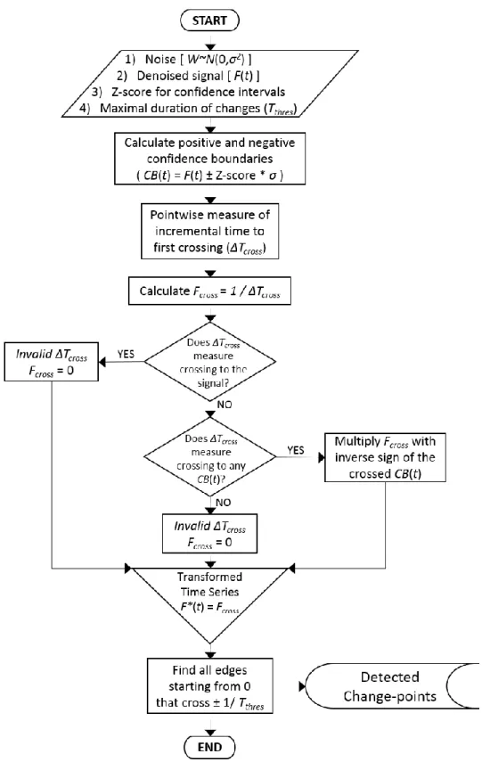
Figure 2.7. Flowchart of the slope threshold algorithm used to detect changes in time series. ... 33

Figure 2.8. Illustration showing the slope threshold algorithm. ... 34

Figure 2.9. Relative fluorescent changes of two hypothetical Ca2+ indicators similar to OGB1 ... 36

Figure 2.10. Illustration of the modeled system from the in vivo imaging experiments. ... 37

Figure 2.11. Illustration of the theta transformation model (𝛳trans) modifying the kernel response to a single action potential spike. ... 39

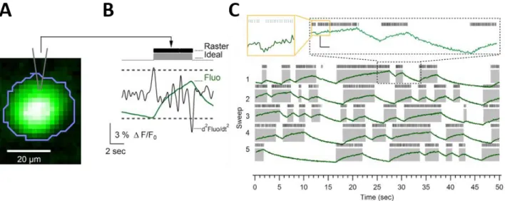
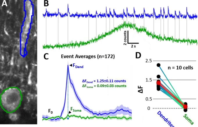
Figure 3.1. Somatic calcium dynamics relay the simple spike activity ... 41

Figure 3.2. Somatic calcium signals are linearly related to firing frequency changes of simple spikes. .... 44

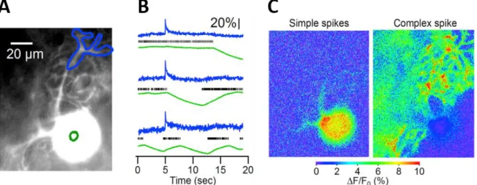
Figure 3.3. Comparison of Complex vs Simple Spike calcium signals in the Purkinje cell soma. ... 45

Figure 3.4. GABAA receptors correlate activity between direct Purkinje cell neighbors in the same sagittal plane. ... 49

Figure 3.5. Simultaneous recordings of in vivo cell-attached patch clamp and GCaMP6f calcium imaging in Purkinje cell somas ... 52

Figure 3.6. Somatic vs. Dendritic Ca2+_{images with GCaMP6f in anesthetized animals. ... 55}

Figure 3.7. Two-photon calcium imaging of cerebellar Purkinje cell somas expressing viral GCaMP6f in anesthetized mice. ... 56

Figure 3.8. Example of the slope thresholding algorithm in action. ... 57

Figure 3.9. Assessment of the average spontaneous activity in Purkinje cells on anesthetized animals. ... 58

Figure 3.10. Running wheel experiments with 2-photon calcium imaging of an L7-Cre mouse with GCaMP6f expression in cerebellar Purkinje cells. ... 60

(17)

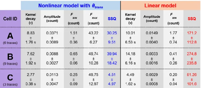
Table 2.1. Bicarbonate-buffered external solution (BBS). ... 14 Table 2.2. HEPES-buffered external solution (HBS). ... 14 Table 2.3. Internal solution for Ca2+_{imaging in slices. ... 16} Table 3.1. Estimated parameters of the fitted models from the simultaneous cell-attached and calcium

(18)

1

1. INTRODUCTION

To cope with a changing environment, animals must form accurate representations of their context using their sensory inputs, so they can change their behavior accordingly. However, the self-generated stimuli produced by an animal’s engagement with its environment (known as reafference) gets mixed with the external stimuli, thus confounding the relevant information needed to adjust its behavior. One option to minimize this confusion might be attained by comparing the animal’s sensory input with other sources of information of the animal’s own activity. Such extra information could come from copies of motor commands (known as corollary discharges). In principle, this additional information could be used to predict and nullify the effect of the self-generated stimuli so the external signals stand out. However, it is still unclear whether and how the brain of highly evolved vertebrates is able to make such computations (Sawtell, 2017).

1.1. Primitive behavior correction based on sensory prediction: Cerebellum-like structures Some independent evolutionary threads in the animal kingdom have maintained simpler versions of sensory systems that have to deal directly with this reafferent cancelling of self-generated sensory stimuli. One well studied example is the electrosensory system in aquatic animals like in some elasmobranchii (sharks and rays, e.g. Bodznick, Montgomery, & Carey, 1999), gymnotids (knifefishes; MacIver, Sharabash, & Nelson, 2001), mormyrids (eg. elephant fish; Baker, Kohashi, Lyons-Warren, Ma, & Carlson, 2013) and even in mammals such as monotremes (Langner & Scheich, 2009). These animals are capable of locating the bioelectrical fields generated from living creatures in water through two types of electrolocation systems: (1) a passive sensing system constituted from ampullary electroreceptors and (2) an active system employing the perturbations created from a specialized electric organ sensed by tuberous electroreceptors. Both types of electrolocation are affected by the animal’s own bioelectric fields (e.g. cardiac and ventilatory pulses), the movements of its receptors relative to itself (e.g. lateral line deformation while swimming), and their own electric organ discharges (EODs) for animals with active electrolocation (Sawtell, 2017).

Interestingly, there is a common feature among these electrosensory animals regarding the processing of their electroreceptor signals. Convergence of the electrosensory input with the

(19)

2 streams of additional information from the animal’s behavior occurs in a brain structure similar to the mammalian cerebellum (Bell, Han, & Sawtell, 2008). In general, these cerebellum-like structures have one layer containing bundles of fibers running parallel to each other that carry the information predicting the sensation (like corollary discharges or proprioception). These parallel fibers establish excitatory synapses with the arborization of principal cells, which also receive peripheral electroreceptive input. The region where parallel fiber and principal cellss intersect is called the molecular layer, which usually contains inhibitory interneurons also connected to the parallel fibers (Golgi and stellate cells). The origin of the parallel fibers can be traced down to small cells located in a region called the granule layer.

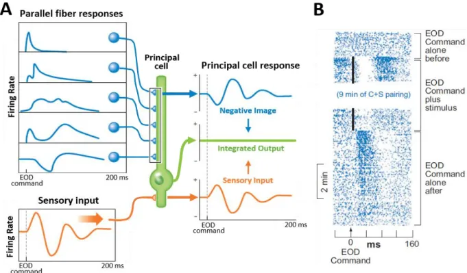
Inside the principal cells, the combination of all the parallel fiber activities in their dendrites generates a signal that exactly opposes the sensory input coming from the electroreceptors when there is no external stimuli, creating what is called a negative image (Fig. 1.1.A). Thus, as elegantly demonstrated by Curtis Bell in the 1980s, when both the negative image and the sensory input collide in the principal cell, the output of the cell will only reflect the perturbations of the signal attributed to external sources (Bell, 1981). Moreover, the negative image could be readjusted via the plasticity of the parallel fiber responses in the principal cell to match new trends in the sensory inputs. This has been demonstrated by pairing artificial electrosensory stimuli to the central predictive signals in electroreceptive animals. For instance, in the mormyrid fish a pairing between its EOD motor command and an external electrical stimulus in its environment causes its ampullary receptors (the principal cells) to adapt their output so they stop responding to the new artificial trend. Once the pairing is halted, the ampullary receptors exhibit a response of opposite sign to the previous artificial stimulus, which in turn also fades eventually (Fig. 1.1.B).

In this way, the cerebellar-like structures could be though as adaptive filters that enrich the behaviorally relevant cues from the environment against the irrelevant background of sensorial trends, including reafference signals. The key feature of this filter is the production of a precisely-timed negative image, which requires a complex array of both excitatory and inhibitory signals that shape the response of the principal cells (Sawtell, 2017). To achieve this purpose, there exists subsets of interneurons inside the cerebellar-like structures that can modify the parallel fiber information: unipolar brush cells, Golgi cells, and stellate cells (Montgomery & Bodznick, 2016). The role of unipolar brush cells is to interconnect groups of granule cells via excitatory synapses, hence unifying the parallel fiber response on downstream targets. On the other hand, Golgi and

(20)

3 stellate cells are inhibitory cells embedded in the granule and molecular layer respectively. The function of their inhibition is to convert the excitatory signals coming from the parallel fibers into an opposite inhibitory version that allows for a change of the signal polarity. This enables the feedforward (or common-mode) rejection of some predictive information sources by cancelling their signals with their self-activated inhibitory counterpart. Additionally, if the inhibition activated by the feedforward mechanism surpasses the excitatory effect on the principal cells, the result could be a signal with a completely reversed polarity. This increases the effective dynamic range available for the negative image to cancel out the sensory input in the principal cells (Montgomery & Bodznick, 2016).

Figure 1.1. Negative image formation in the cerebellar-like structures of active electrosensory organs.

Note: A. Cancellation of a sensory input with its negative image assembled from the parallel fiber inputs in a principal cell. B. Raster display of the extracellular action potentials recorded in principal cells (receiving ampullary afferents) located in the electrosensory lobe of a mormyrid fish subjected to artificial electric stimulation. The EOD motor command initially has no effect on the cell. An electrosensory stimulus (vertical black line) that evokes a pause-burst response is then paired with the command. After several minutes of pairing, the stimulus is turned off and a response to the command alone is revealed, which was not present before the pairing and which is a negative image of the previously paired sensory response. Images adapted from Bell et al., 2008; Sawtell, 2017.

(21)

4

1.2. Parallelism of the cerebellum-like structures with the mammalian cerebellum

The many similarities between cerebellum-like structures and the mammalian cerebellum suggest that the latter may also be involved in generating predictions concerning expected sensory input or states of the system (Bell et al., 2008). First, the histological composition of both nervous centers is almost identical. The two possess molecular and granule cell layers with principal cells embedded in the molecular layer, that in the cerebellum are called Purkinje cells (PCs). Also, the inhibitory and excitatory interneurons like unipolar, Golgi and stellate cells are present in both organs. However, the cerebellum presents some peculiarities. It has a specialized type of stellate cells called basket cells (Castejón, 2003), which connect to PC somas through processes resembling a “basket” (hence their name). Additionally, Purkinje cells in the cerebellum connect to an additional excitatory fiber that climbs around the dendritic arborization of the cells. This climbing fiber comes from a brainstem region called the inferior olive nucleus (Palay & Chan-Palay, 1974). Typically, Purkinje cells have thousands of glutamatergic synapses with multiple parallel fibers, but only one climbing fiber makes glutamatergic synapses on an individual PC. Moreover, the cell processes (dendrites, axons) of the elements in the molecular layer of the cerebellum are strictly oriented in the sagittal plane, and perpendicular to the parallel fibers (see Fig. 1.2. for more details).

Secondly, the circuit physiology of the cerebellum and cerebellum-like structures is also very similar. The most crucial matching is that between the inputs received by the two organs. Both of them take in parallel fibers that convey a rich variety of information from multiple sources (sensory and/or highly cognitive inputs). Also, both receive a secondary input (from peripheral sensors in cerebellum-like structures and from climbing fibers in the cerebellum) that relays specific information which subdivides the set of principal/Purkinje cells that share the same parallel fiber inputs (Bell et al., 2008).

Thirdly, several studied functions associated to the cerebellum are akin to the functions analyzed by the adaptive filter framework in cerebellum-like structures. The most classical example is the vestibulo-ocular reflex (VOR) researched from the mid 1970’s (Ito, 2012). In the mammalian VOR model, the cerebellum has a direct influence in the reflex pathway that adjusts the eye position whenever the head movements cause an image to sweep across the retina (also called ‘retinal slip’). The movements of the head are reported by the vestibular system on the inner

(22)

5 ear in mammals. The nature of this model is that the proprioception of the head is used to reduce errors in an unrelated sensory modality such as vision, in an open-loop fashion that requires a transformation of one sensory modality to another. This open-loop compensation, having both the predictive information from the vestibular system and the motor command of the eye muscles reaching the cerebellum, is an echo of the adaptive filter operation already described for electrosensory fishes (Dean, Porrill, Ekerot, & Jörntell, 2009).

The predictive capability demonstrated by the cerebellum and cerebellum-like structures have led to the hypothesis that they implement forward control models (Sawtell, 2017). In these models, both the motor commands and the current state of the system (like appendage positions or velocities) are used to predict the system’s future state. By comparing the predicted and the actual system states (i.e. cancelling the negative image with the sensory input), an error signal is computed and is fed back to the generator of the motor command, thus correcting its inaccuracies for the next action. Then again, for this model to be adaptable in face of sensory changes, it requires synaptic plasticity inside the cerebellar elements as shown already with the adaptive filter. One advantage of forward models is their ability to explain fast and coordinated movement sequences, given that feedback from peripheral sources is very slow (Bell et al., 2008). To a certain extent, the forward model can also explain classic symptoms of cerebellar degeneration, like the uncoordinated tremors while doing precise motor tasks, or the inability to rapidly adjust the motor commands to abrupt and steady changes in sensory inputs. Forward models are also successfully applied in robotics to implement motor control algorithms (Floreano, Ijspeert, & Schaal, 2014). Despite the compelling evidence in its favor, the top-to-bottom perspective of this model still lacks the explanation of the cellular and circuit mechanisms that originate its cerebellar computing properties.

(23)

6 Figure 1.2. The mammalian cerebellum: histology, cellular connectivity

and the cerebellar cortex motif.

Note: A. Illustration of a mouse adult cerebellum. A uniform layering of cell types can be found throughout the vermis and more lateral hemispheres (shown in schematic parasagittal section): the Purkinje cells layer separates the molecular layer from an internal granule cell layer. Deep cerebellar nuclei (GABAergic and glutamatergic neurons) lie within the white matter. B. 3-D illustration of the crystal-like structure of the cerebellum. Purkinje, stellate and basket cells in the molecular layer have their processes constrained to parasagittal planes. Purkinje cells receive input from the numerous and densely packed parallel fibers that run at right angles to the Purkinje cell dendrites and make up the bulk of the molecular layer. Parallel fibers are the axons of the billions of granule cells that make up the bulk of the cellular layer beneath the Purkinje cells. Granule cells receive input from many parts of the brain via the mossy fibers. Climbing fibers are the only other input pathway. C. Schematic circuit diagram of the cerebellum. Mossy fiber inputs branch from the cortex, as do climbing fibers from their origin in the inferior olive. Both converge with Purkinje cell outputs onto the deep cerebellar neurons. D. The cerebellar cortex motif further simplified: the mossy fiber / granule cell / parallel fiber / Purkinje cell pathway is illustrated. The true complexity of the connectivity would be better shown by having 100,000 mossy fibers and 4.6 million granule cells on the input side for the single Purkinje cell output neuron. Given these ratios, it is apparent that granule cells make up the majority of cells in the cerebellum, but also that the input pathway goes through an information expansion step between mossy fibers and granule cells. Image adapted from (Basson & J Wingate, 2013; Montgomery & Bodznick, 2016).

(24)

7

1.3. Cerebellar dynamics elucidated through electrophysiological experiments

In the search for linking the cerebellar circuit dynamics and its emergent functional attributes, many authors have studied the cerebellum using a variety of methods. Initially, most of the research at the cellular and circuit levels was done using electrophysiological techniques in acute models, like decerebrated cats or cerebellar slices. The biggest exponent on these initial stages was the Eccles´ research group in the 1960s, located in the University of Canberra (Australia). By using intracellular recordings with glass microelectrodes and complementing with electron microscopy, they identified the elements responsible for glutamate-mediated excitation (granule cells, mossy and climbing fibers) and GABAergic inhibition (basket, stellate, Golgi and Purkinje cells) in the cerebellum (Palay & Chan-Palay, 1974). At the end of that decade, their findings were synthesized in the first theoretical model of the cerebellar cortex circuitry by both Marr and Albus (1969-1971), which predicted the relevance of synaptic plasticity as a memory element involved in cerebellar learning. Later, some of the model predictions were supported by the finding of long-term depression (LTD) in synapses between parallel fibers and Purkinje cells (Ito & Kano, 1982). This bottom-to-top approach was a phenomenal start for explaining cerebellar physiology, that led directly to the research of its connection to behavior (as the VOR model). However, the model made many assumptions on the cellular physiology in the cerebellum that had to be tested.

As Purkinje cells were found to be the main target of the inputs reaching the cerebellum, and with their size facilitating electrode recordings, most of the initial cellular research of the cerebellum has focused on understanding how these cells relay information in the cerebellar cortex. The most productive researcher in this field has been Rodolfo Llinas, who studied in detail the electroresponsiveness and related ionic conductances of these cells (Llinás & Sugimori, 1992). In his experiments, he found a clear difference between the somatic and dendritic compartments of Purkinje cells. For instance, dendrites had responses to inputs associated to Ca2+ conductances, whereas the soma had all-or-nothing responses associated to Na+ conductances (Llinás & Sugimori, 1980a, 1980b). Their work led to the understanding of the electric effects that inputs have on the Purkinje cells, which are separated into three types: (1) the electrotonic contribution of excitatory and inhibitory potentials from parallel fiber and interneurons synapses, (2) the all-or-none Ca2+_{-dependent spikes in the dendrites generated by climbing fibers (named complex spikes;}

(25)

8 CS), and (3) the Na+_{-dependent action potentials in the somas (named simple spikes; SS)}

modulated by the balance between inhibitory and excitatory inputs.

One of the biggest surprises encountered with Purkinje cells was that they transmitted a GABAergic output to distant cells inside the cerebellum, into a region called the deep cerebellar nuclei (DCN; see Fig. 1.2.C). The convention at that moment was that long cell projections in the nervous system were all excitatory (Ito, 2012). Moreover, it was known that Purkinje neurons outnumber the cells in the DCN at least by an order of magnitude, meaning that multiple PCs inhibit a single DCN cell (Fig. 1.3.). Since Purkinje cells have a high baseline activity in vivo, it is a challenge to reconcile how this massive inhibition from populations of PCs can modulate the activity of its DCN targets. More recently, experiments using dynamic clamp techniques to simulate PC inputs over recorded DCN cells have given insights over this conundrum (Gauck & Jaeger, 2000; Person & Raman, 2012). What appears to allow the DCN cell output to overcome this inhibition is an interplay between the synaptic weight of the PC-DCN synapses, the synchronicity of the PC inputs and the assembled silent periods from the PC activity (with the resulting effects depicted in Fig. 1.3.C). As a consequence of this population effect of PCs into DCN cells, there is a need to record activity simultaneously from multiple Purkinje neurons in the cerebellum to elucidate the type of information that is conveyed to the DCN.

Figure 1.3. Convergence of Purkinje cells GABAergic output into the deep cerebellar nuclei

(26)

9

Note: A. Diagram representing the connection of multiple Purkinje cells onto a single DCN cell. The most recent estimation of the PC-DCN effective convergence ratio (in mouse) is of maximum 30:1 cells (Person & Raman, 2012). B. Reconstruction of the axonal projections of Purkinje cells in the cerebellum of mice visualized in horizontal planes. Top: Purkinje cells on the same sagittal plane (visibly overlapping in this horizontal perspective) with their axons reaching the same spot in the deep nuclei. Bottom: Two pairs of Purkinje cells from another region. PCs on contiguous sagittal planes (non-overlapping cell bodies) have their projections reaching different deep nuclei regions, adapted from Sugihara Izumi et al., 2008 C. Schematized spike rasters showing the key features of three non-mutually-exclusive models of Purkinje cell regulation of nuclear cell firing. Nuclear cell spikes reflect responses to three afferent Purkinje cells. Inverter, nuclear cell firing rate varies inversely with the assembled Purkinje cell firing rate. T-type rebound, nuclear cells are largely silenced by Purkinje cell activity, but fire bursts of action potentials driven by low-voltage-activated Ca2+_{currents when Purkinje cells stop firing. Synchrony code, nuclear cells are} silenced by asynchronous inhibition but produce short-latency spikes after IPSPs from synchronous inputs (adapted from Person & Raman, 2012).

1.4. Calcium imaging as a research tool for studying the cerebellar circuit dynamics Although electrical recording offers high temporal resolution with outstanding signal to noise ratios, it is an invasive technique that damages the cerebellar tissue and that cannot acquire data from a high number of cells. Even advanced electrophysiological recording techniques, such as tetrodes and multielectrode arrays, cannot record cells just a few microns far from their sensitive sensors and cannot distinguish the absolute positions of the cells responsible for the signals (Harris, Quian Quiroga, Freeman, & Smith, 2016). However, with the advent of imaging methodologies neuroscience has developed alternative measurements of activity using fluorescent indicators that allow less invasive experiments and a higher number of cell recordings, albeit with a loss of signal time precision. Nowadays, the most used probes for imaging are the calcium indicators, since calcium is an intracellular messenger that has an essential role in neuronal communication, e.g. synaptic transmission with voltage-activated calcium channels (Grienberger & Konnerth, 2012). There are two types of fluorescent Ca2+ indicators typically used for neuronal imaging: the chemical indicators and genetically encoded calcium indicators (or GECIs).

Commonly used chemical indicators are Oregon Green BAPTA-1 (OGB1) and fura-2, as both the brightness and the Ca2+ binding properties from these indicators make them well suited for recording in neurons. First, they have KD values just above the normal Ca2+ baseline

concentration of cells (50-100 nM), allowing a good usable range of their Ca2+-dependent fluorescence changes. Second, they have only one binding site to Ca2+, which simplifies the decoding of fluorescence changes into calcium changes. And in the case of fura-2, there is a shift in wavelength emission upon Ca2+ binding that can be used to obtain a ‘ratiometric’ of the real

(27)

10 intracellular Ca2+_{concentration. Nevertheless, one disadvantages of chemical indicators is that}

they have to be loaded into cells. Some synthesized variants of these indicators facilitate the loading process by using an acetomethylester (AM) functional group that confers liposolubility to the molecule. These lipophilic variants are then perfused on the cells of interest so they can cross the cell membrane. Once inside the cell, the endogenous activity of internal esterases cleaves the -AM radical and frees the original hydrophilic compound, effectively trapping it inside the cell (Takahashi, Camacho, Lechleiter, & Herman, 1999).

The other type of Ca2+ indicators widely used in imaging are GECIs. These indicators are chimeric proteins designed from the fusion of functional blocks present in other calcium-sensitive and fluorescent proteins. The most recognized family of GECIs are GCaMPs (currently in their sixth iteration; Chen et al., 2013; Helassa, Podor, Fine, & Török, 2016). These proteins are composed of parts of the jellyfish’ green fluorescent protein (GFP), the Ca2+_{binding motif of}

calmodulin, and a peptide coming from a myosin light chain kinase (M13); the last “P” stands for protein (Nakai, Ohkura, & Imoto, 2001). The main advantage of these indicators relies in their proteinic nature, as they can be conveniently encoded into artificial genes for cell expression. At the moment, four methods are used to express the GCaMP gene with a cell-specific transcription promoter: (1) in utero electroporation of a plasmid containing the GCaMP gene, (2) creation of a transgenic animal line, (3) transfection with a viral construct encoding the gene (M. Z. Lin & Schnitzer, 2016), and (4) a combination of the two previous methods using a site-specific recombination system (e.g. Cre/Lox) to ensure specificity of the expression (Sługocka, Wiaderkiewicz, & Barski, 2017). Currently, the most used GECI in the Ca2+ imaging domain is GCaMP6f (Hudson, 2018). Its brightness and Ca2+ affinity are very close to commonly used chemical indicators like OGB1 (Yamada & Mikoshiba, 2016). So, an obvious question arises: which one should be chosen as a reporter of Purkinje cell activity?

Each Ca2+ indicator has both advantages and disadvantages. The expression systems for GCaMP6f allows for targeted “loading” of the indicator in very specific cell-types in vivo. In contrast, the alternative method using perfusion of OGB1-AM (multibolus loading) unselectively labels all cells and cellular compartments where the molecule can diffuse, resulting in less contrasted images with more heterogeneous loading of the indicator (Franconville, 2010; Sullivan, Nimmerjahn, Sarkisov, Helmchen, & Wang, 2005). This impairs the quality of the imaging to resolve genuine signals above the background noise (Wilt, Fitzgerald, & Schnitzer, 2013).

(28)

11 Moreover, chemical indicators like OGB1 are cleared out from cells over time, whereas ensures the GCaMP6f transgene continuous expression. The latter extends the usable period of the fluorescent cells, enabling chronic experimentation on the animals (Grienberger & Konnerth, 2012). Lastly, our lab has already prior experience working with both methods (Astorga et al., 2015; Franconville, 2010) and it was concluded that the daily multibolus loading of AM compounds attains a less reliable labeling of the cells. Comparatively, the GCaMP expression system was more efficient. In the case of this thesis, there was an extra advantage of using GCaMP since the modified mice lines and viruses used for those previous projects were available in our lab. However, despite these advantages of GECIs there is a major complication. Current GECIs show a steep non-linear response to calcium that distort the fluorescence signals at both low and high calcium concentrations (Chen et al., 2013; Eilers, Callewaert, Armstrong, & Konnerth, 1995; Kano, Rexhausen, Dreessen, & Konnerth, 1992), whereas organic indicators only present nonlinearity at high calcium levels. Although this is an unavoidable difficulty, there are ways to extract information from these distorted signals that will be discussed below. For the moment, even with the notorious nonlinearities of GCaMP6f, this calcium indicator is able to report moments of high or low activity in cells in vivo.

The advantages of in vivo Ca2+_{imaging are well-suited for studying the populational}

information of neurons in the cerebellum. To date, this method has been more frequently applied to monitor the Ca2+_{signals associated to the activity of granule cells (deep in the cerebellar cortex)}

and Purkinje cell dendrites (on its surface) via 2-photon microscopy (Gaffield, Amat, Bito, & Christie, 2015; Giovannucci et al., 2017; Najafi, Giovannucci, Wang, & Medina, 2014a, 2014b; Ozden, Dombeck, Hoogland, Tank, & Wang, 2012; Zariwala et al., 2012). However, there are very few studies focused on the cells between this two depths of the cerebellar cortex, such as the molecular layer interneurons (MLI; Astorga et al., 2015; Franconville, Revet, Astorga, Schwaller, & Llano, 2011) and Bergmann glial cells (Hoogland & Kuhn, 2010). Surprisingly, there is no publication with in vivo recordings of spontaneous Ca2+ imaging in Purkinje cell somas, considering their pertinence in the integration of the cerebellar cortex output. This lack of information might have been caused by the indications that PC somas have very small calcium signals in response to direct depolarization (Callewaert, Eilers, & Konnerth, 1996; Eilers et al., 1995; Gruol, Netzeband, & Nelson, 2010; Tank, Sugimori, Connor, & Llinas, 1988) or to action potentials triggered by mossy fiber stimulation (Gandolfi et al., 2014) in cerebellar slices.

(29)

12 Nevertheless, in view of the proposal that Purkinje cell pauses are carriers of information to the DCN (instead of the spikes themselves), and considering the current advancements on in vivo techniques and analysis (Theis et al., 2016) that optimize data acquisition and quality, it might be possible to extract functionally relevant information from Purkinje cells somatic Ca2+ imaging.

In this thesis, we test the potential use of somatic calcium imaging in Purkinje cells as a faithful reporter of the cell’s electrogenic output. We also assess the coordination of Purkinje cells predicted by the confined GABAergic connectivity in the cerebellum, which is anatomically organized along sagittal planes.

(30)

13

2. METHODOLOGY

The thesis is separated in two broad sections defined by the experimental methodologies. The first part corresponds to the slice experiments made in rats, which allowed us to extract data with high number of repetitions and with very low confounding variability. The insights obtained from the slice work were used to design experiments with mice in vivo, as they have much more logistical complexity and more difficult interpretation.

2.1. Common consumables

2.1.1. Animals

Rats: Pregnant Sprague-Dawley Rats were bought from Janvier Labs® and kept in a conventional animal house with a normal light-dark cycle (12 h/12 h), with food and water given ad libitum. The newborn rats were left with their mother until the day of the experiment.

Mice: For most of the experiments, two transgenic mice lines with knock-in of a Cre recombinase were used: one with the Cre associated to the expression of the parvalbumin promoter (PV-Cre), and the other through the Purkinje cell specific protein 2 (L7-Cre). The lines were kept in colonies dating from February 2011 (PV-Cre) and June 2013 (L7-Cre) inside the clean room facilities at the University Paris Descartes. The first generation came from strains sold by the Jackson Laboratories™, B6;129P2-Pvalbtm1(Cre)Arbr/J and B6.129-Tg(Pcp2-cre)2Mpin/J respectively.

2.1.2. External solutions

Along the work of this thesis, we used two types of solutions to keep the exterior of the nervous tissue under the closest physiological conditions. A bicarbonate-based solution (BBS) detailed in Table 2.1., and an HEPES-based solution (plainly identified with HEPES solution) described in Table 2.2. For in vivo extracellular recordings and stimulation, a concentrated volume of Alexa 594 (1 M) was added to the HEPES solution to allow for imaging of the electrode with the 2-photon microscope in order to better monitor the position of the electrode. The final concentration of Alexa was 50 µM.

(31)

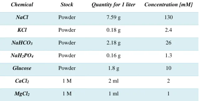
14 Table 2.1. Bicarbonate-buffered external solution (BBS).

Chemical Stock Quantity for 1 liter Concentration [mM]

NaCl Powder 7.59 g 130 KCl Powder 0.18 g 2.4 NaHCO3 Powder 2.18 g 26 NaH2PO4 Powder 0.16 g 1.3 Glucose Powder 1.8 g 10 CaCl2 1 M 2 ml 2 MgCl2 1 M 1 ml 1

Note: The final osmolarity was 300 mOsm. The solution was constantly bubbled with a 95/5 O2/CO2 gas mixture to maintain its pH and thereby avoid precipitation of divalent cations.

Table 2.2. HEPES-buffered external solution (HBS).

Chemical Stock Quantity for 1 liter Concentration [mM]

NaCl Powder 7.71 g 132 KCl Powder 0.3 g 4 NaHCO3 Powder 0.21 g 2 HEPES Powder 2.38 g 10 Glucose Powder 4.5 g 25 CaCl2 1 M 2.5 ml 2.5 MgCl2 1 M 1 ml 1

Note: HCl (1 M) was added to the solution in drops of (~10 µl) until reaching a pH of 7.4. Osmolarity was 300 ± 5 mOsm. The solution was kept frozen at -20°C and thawed when used.

(32)

15 2.1.3. Anesthetic solutions

For general anesthesia the mice were administered via intraperitoneal injections with a solution of ketamine (15 µg per gram of animal) and xylazine (10 µg per gram) diluted in isotonic saline solution and kept at 4°C. For hypodermically administered local anesthesia used in surgeries, we used a mixture of 0.1 ml of lidocaine (20 mg/ml) diluted to 1 ml with saline solution. 2.1.4. Viral solutions

Two lots of AAV2/1.CAG.Flex.GCaMP6f.WPRE.SV40 (100 µl with titer of 7.6e+12 GC/ml) bought from the U. Penn. Vector Core (material transfer agreement) were aliquoted to 5 µl volumes and stored frozen at -80°C. For each viral injection session, a new aliquot was diluted in isotonic saline solution to the following concentrations: PV-Cre animals required a dilution between 1/100 to 1/50 to have a high expression after three weeks of expression L7-Cre animals required higher concentrations ranging from 1/40 to 1/20. The diluted solutions were kept at ~4°C until the time of injection.

2.2. Acute brain slice experiments

2.2.1. Rat cerebellum slice preparation

Sagittal slices from the vermis of rat's cerebellum were prepared using the protocol already established in the lab (Llano, Marty, Armstrong, & Konnerth, 1991). Rats from 11 to 36 days old were sacrificed by decapitation under the anesthetic effects of isofluorane. Then, the cerebellum was carefully exposed from the skull and the vermis was cut apart from the hemispheres with a disposable blade. The dissected vermis was extracted from the tissue with a planar lancet and submerged in ice-cooled (~4°C) BBS solution bubbled with 95% O2 and 5% CO2. The extracted

portion was rapidly cleaned with forceps under a stereoscope to remove the residual meninges adhered to its surface. After cleaning, the tissue was taken out of the solution and glued with cyanocrylate (Loctite® SuperGlue) to a metallic base of a Leica® VT1200S vibratome. Once inside the vibratome, the tissue was again submerged in more cold BBS solution and 200 um slices were cut by advancing the blade at a rate of 0.05 mm/s.

Each slice was taken out of the vibratome stage and put over a resting net inside a heated bath with more bubbled BBS solution at 34°C. The slices were left to recover for 30-45 minutes and then moved to room temperature before performing experiments.

(33)

16 2.2.2. Electrophysiological recordings in slices

The recording chamber was continuously perfused at a rate of 1-2 ml/min with BBS. Recordings were made at room temperature. The Purkinje cell layer and the molecular layer of the cerebellar cortex were visualized using an Axioskop microscope (Zeiss®) equipped with a 63X/0.9 water immersion objective (Zeiss®). Signals were recorded with an EPC-10 amplifier with Patchmaster software v2.32 (HEKA®). Borosilicate glass pipettes were pulled using a two-step vertical pipette puller (HEKA® PIP6) and had an open tip resistance of 3-5 MΩ for cell-attached and whole-cell recordings. The cell-attached recordings were made in voltage clamp mode with BBS in the pipette and 0 mV holding potential.

For experiments in which GABAA receptors were blocked with antagonists, the normal

BBS used in the bath perfusion was changed to a BBS containing gabazine diluted to 10 µM. 2.2.3. Calcium imaging in slices

Purkinje cells were loaded with internal solution containing diluted OGB1 (see Table 2.3.) through a whole-cell voltage clamp for ~20 minutes, then the pipette was retracted slowly. When the leak currents where minimal and only the capacitive currents remained (indicating the initiation of an outside-out patch), the pipette was retracted faster and the membrane resealed, thereby trapping the indicator inside. Probe-loaded cells were illuminated with a 470 nm LED controlled with an Optoled system (CAIRN®). Light from the LED was sent down the epifluorescence pathway of the microscope and reflected off from a T495LP dichroic mirror (Chroma™) onto the preparation. Then, the fluorescence signal coming from the sample passed through the mirror and an emission filter (Chroma™ ET525/50M), before it was detected with an ANDOR® iXON CCD camera (model 887) at a frame-rate of 31.5 Hz.

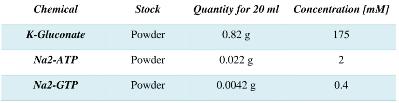
Table 2.3. Internal solution for Ca2+ imaging in slices.

Chemical Stock Quantity for 20 ml Concentration [mM]

K-Gluconate Powder 0.82 g 175

Na2-ATP Powder 0.022 g 2

(34)

17 Chemical Stock Quantity for 20 ml Concentration [mM]

HEPES Powder 0.048 g 10

EGTA Powder 0.0076 1

CaCl2 1 M 2 µl 0.1

MgCl2 1 M 48 µl 2.4

Note: KOH (1 M) was added in drops of 10 µl until the solution reached a pH of 7.4. Osmolarity was 327 ± 5 mOsm. The solution was frozen at -20°C and thawed when used. Oregon Green BAPTA-1 solution (OGB1, 1 M) was added to get a final probe concentration of 50-100 µM with a ~ 10% dilution of the internal solution.

2.3. In vivo experiments

2.3.1. Two-photon imaging

Two custom-made set-ups were used for scanning 2-photon imaging, each of them adapted for experiments in anesthetized or awake animals; however, both shared the same basic configuration (Fig. 2.1.A). A Ti-Sapphire laser from SpectraPhysics® was employed as a high-power source of infrared laser. The laser was conducted with Thorlabs® mirrors into a Pockels cell where its intensity was modulated (ConOptics™ 350-80BK with amplifier 302RM). The resulting light was expanded with a telescope made of Thorlab® lenses to decrease the beam density and it was directed to a set of two mirror galvanometers (Cambridge Technology™ Galvanometer XY Set model 6221H) to modify the X and Y positions of the beam in the sample’s optical plane. Then, the laser light passed through a dichroic mirror (Chroma Technology™ 670DCXXR) with a cut-off wavelength of ~ 670 nm and went into a water immersion objective (Olympus® XLUMPlanFL-N 20x/1.00 W). The measured point-spread function (PSF) of the microscope had a full width at half maximum (FWHM) of 1 µm in the X and Y dimensions, and 10 µm in the Z direction. In a region inside this volume, the sample is bathed with a high enough density of photons to allow the 2-photon excitation of the fluorophores. The absorbed energy in these molecules is then released with an Stokes shift, emitting a photon with a lower energy than the total energy absorbed, but that has a higher wavelength than the excitation light. The fluorescent light gets scattered while traversing the sample, and some of it is captured by the objective. The incoming light from the objective passes again to the dichroic mirror, and only the

(35)

18 short wavelengths produced by the fluorophores are reflected to a Photomultiplier tube (Hamamatsu® PMT H7422-40). The resulting electrical signals from the PMT were transformed into ultra-fast digital pulses by an edge detector (Hamamatsu® C9744). Such pulses were individually counted by a National Instruments® card (NI - BNC2090A) and sent to a desktop computer. The data was processed using Igor Pro 6.37 with the “NIDAQ tools MX” external operation software, in conjunction with the Igor2P repository developed by Brandon Stell, (Stell, 2015/2018).

To easily locate the positions of interest on the surface of the animal for the imaging, an additional hot or cold mirror (BrightLine® FF735-Di02-50x36) was put between the galvanometers and the dichroic mirror to extract some of the incident light into an USB camera (PCO® Pixelfly, or Thorlabs® DCC1545M). An extra light source (any general lamp) was used to illuminate the tissue.

Over the course of this thesis, a device to add more I/O control to the Hamamatsu® PMT was made available (M13414). This device allows software control of the PMT over-voltages, which are dangerous to the equipment and occur regularly while doing in vivo imaging. However, no power supply nor interface were included on the product. So, a simple circuit was designed to add these functional blocks, plus protection circuits. The design was manufactured and tested in real experiments.

Two different software were used as the graphical interfaces to control the devices, make real-time images and record the signals. For the experiments using anesthetized animals, the set-up available worked with Igor Pro 6.37 (Wavemetrics™) with the Igor2P module (Stell, 2015/2018). For the experiments with awake animals, the set-up used the open-source Python-based platform of ACQ4 (Campagnola, Kratz, & Manis, 2014). Both programs were capable of I/O control of all devices through the NI card.

2.3.2. Behavioral set-up components

The set-up used for awake experiments had some additional features that were fundamental for its imaging capability and behavioral tests. First, the stability of the mouse’s head was critical to reduce movement artifacts while imaging. The best arrangement consisted of a structure of two Ø 2.5 cm steel columns holding a Ø 1.3 cm horizontal bar in the front of the animal, while a secondary Ø 1.3 cm steel column with an angle clamp was used on the back (all from Thorlabs®).

(36)

19 In the middle of the horizontal bar, there was a customized pressure clamp designed to restrain the headpieces of the mouse. An extra metal piece was cemented to the animal on the back of its head to improve stability by clamping it to the secondary back column.

The other additional feature in the set-up was the use of a 3D-printed plastic wheel with a mesh flooring, so that the animal could run while imaging its cerebellum. The wheel was positioned in the center between the steel columns, at an optimized position to allow the access of the immersion objective to the animal (see Fig. 2.1.C). The movements of the wheel were captured using a rotary encoder (CUI Inc.™ AMT112S-V) attached to the rotation axis of the running wheel, and directly connected to the NI card.

(37)

20 Figure 2.1. Experimental set-up configurations.

Note: A. Diagram showing the basic functional structure for the scanning 2P microscope with photon counting. B. Set-up arrangement for experiments with the anesthetized animal. C. Set-up arrangement for behavioral experiments. 1: Horizontal metallic bar, 2: Objective, 3: Electrode holder, 4: Platform with thermal pad, 5: Pulse oximeter, 6: Back clamp, 7: Running wheel.

(38)

21 2.3.3. Viral injections in mice

Transgenic animals (PV-Cre and L7-Cre) between 40 and 60 days old were anesthetized by intraperitoneal injection (IP) of ketamine/xylazine (see Solutions above). After 5-15 minutes, once the effect of the anesthesia lulled the animal and it didn't move voluntarily, its head was shaved with a disposable surgical blade and then the animal was mounted in a stereotaxic frame. It was of utmost importance to restrain the head of the animal tightly on the frame to avoid mechanical displacements for the next steps. No additional oxygen could be provided to the animal throughout the procedure because the clamps of the stereotaxic frame blocked the access of our ventilation mask to its nostrils. The level of anesthesia in the animal was checked from time to time by the involuntary muscle contractions in response to mild pinches given to its posterior paws. Given that the ketamine/xylazine combination produces a dysregulation of the autonomic system in rodents (Gaertner, Hallman, Hankenson, & Batchelder, 2008), accompanied with a low metabolic rate from subsequent mild hypoxia, the anesthetized animal was kept at around 34°C. At this temperature, the thermoregulatory disorder caused by ketamine might be reduced (M. T. Lin, Chen, & Pang, 1978) and is not too hot to cause unwanted effects such as heat spikes or accelerating the metabolism of the animal leading to more hypoxia. The animal's temperature was maintained by a system of a rectal thermistor and heat plate controlled from an FHC® DC Temperature Controller.

With the animal on position, its head was cleaned with iodine solution (Betadine®) and a sagittal cut on its skin was made to uncover both the parietal, interparietal bones, and a third of the trapezoidal muscles (just above of the occipital bone). To ease the accessibility for the upcoming steps, the insertions of the neck muscles (trapezoidal, splenius and semispinalis muscles) were partly cut and the muscles were put aside with an absorbent cotton tip. When strong hemostasis was needed, various hemostatic composites were used (Ethicon® Surgicel, Bloxang®).

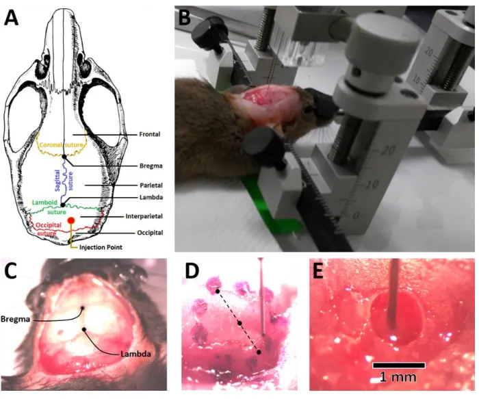
Once the skull was exposed, the tilt of the head was corrected by leveling the coordinates of the bregma and lambda positions with the stereotaxic caliper (Fig. 2.2.). Using the adjusted bregma as an origin, the position around X = 0.5 mm, Y = -5.5 mm was marked which corresponds to the right side of the cerebellar lobule V. As the measurements of the animals were variable, another criterion was used to confirm this position by re-locating the Y coordinate at least 0.5 mm more anterior to its projection from the occipital suture (Fig. 2.2.A). On the chosen position, a hole

(39)

22 of diameter ~ 0.8 mm was drilled with an spherical drillbit of 0.5 mm using a Dremel® rotary tool. The hole was made deep enough to reach the dura mater, it was cleaned from all remainder bone pieces using fine tweezers and the dura was softly pierced with a syringe needle.

Figure 2.2. Viral injections on mice.

Note: A. Anatomical illustration of the main stereotaxic features used to position the injection point. Original from (Geoface, 2016). B. Photo of an anesthetized mouse held by the stereotaxic frame while being injected. C. Close-up to the exposed skull identifying the bregma and lambda positions. D. Example of a marked area prepared for viral injection + chronic window procedures. Diameter of 3 mm, 25x magnification. E. Injecting needle inserted through the drilled craniotomy at 40x magnification. Zoomed images taken with a Leica® Stereoscope MS5.

Through the opening, a WPI™ beveled needle of gauge 34 (with ~200 µm diameter) pre-loaded with 2 µl of viral solution (see Solutions) was inserted into the cerebellar tissue down to a depth of 450 µm. Extra attention was taken to ensure that the needle was getting inside the cerebellum and not only pushing the meninges, which is seen as a small tensile displacement on

(40)

23 the surrounding tissue. After some seconds, the needle was raised 100 µm and then 1.5 µl of viral solution were pumped at a flux of 0.1 µl/min using the hydraulic pressure of a water-filled propylene tube connected to a Hamilton® microliter syringe, in turn pushed by a Harvard Apparatus® pump model 11 Plus. Once finished, the needle was kept on the tissue for some minutes and then carefully removed.

The procedure was ended by suturing the skin wound with a resorbable thread (Ethicon® Vicryl Rapide). The animal was removed from the stereotaxic frame and put under an incandescent lamp until it recovered consciousness. In the meantime, a hypodermic injection of isotonic saline solution was given to the animal to compensate for dehydration and/or loss of blood volume during the procedure.

2.3.4. Anesthetized (acute) experiments

Transgenic animals expressing GCaMP6f for 2-3 weeks after their viral injection were anesthetized with an IP of ketamine/xylazine. Once the animal was deeply anesthetized, its head was shaved, and its skin antisepsis was done with iodine solution (Betadine®). Then, the skin between its ears was cut off to expose the parietal and interparietal bones. All the muscle insertions of the neck were gently detached with a microblade, and the remainder connective tissue was cleaned off. Special care had to be taken when cleaning the injection site, as it was still on recovery and very soft.

The head of the animal was glued with dental cement to a steel bar and secured in a metallic base as shown in Fig. 2.3. As soon as the animal was fixed, a mask with a constant oxygen flow of 1 cm3/s was put on the animal and its blood oxygen saturation was monitored using a pulse oximeter (Starr™ MouseOx). Also, the animal’s temperature was kept at 37ºC with a closed-loop controller (FHC® DC Temperature Controller). Once stabilized, a pool of cement (bigger than the immersion objective for imaging, see 2P Imaging) was made to allow the exposed cranium to be covered in HBS solution. While the skull was still dry, an aperture of ~ 2x3 mm was drilled to expose the cerebellum with its injection point on a side. Then, the area was washed profusely with HBS solution to clean the debris. The bone lid was removed slowly, as the healing tissue from the injections was always tightly adhered to the skull. Most of the time some bleeding started as soon as the bone was removed, which was held off by hemostatic composites (Ethicon® Surgicel, Bloxang®) and cotton tips.

(41)

24 Figure 2.3. Anesthetized (acute) experiments on mice.

Note: A. Photo showing the set-up for holding the mouse and the dental cement pool used to keep its craniotomy immersed in solution. B. Magnified photo (25x) of the craniotomy showing is overall size and location. C. Diagram showing the procedure to position the electrodes inside the cerebellum (description in text).

Usually, a portion of the meninges got ripped off from the injection point in the process of opening the skull. That area was not used in experiments. For procedures requiring cell-attached recordings of Purkinje cells and extracellular stimulation of parallel fibers, the meninges were completely removed using a fine lancet and the craniotomy was covered with agar (0.04 g/ml) made with HBS solution (see Solutions). Once finished, the animal was positioned on the 2P imaging set-up to conduct the experiments (Fig. 2.4.B).

(42)

25 2.3.5. In vivo cell-attached recordings with calcium imaging

To perform a simultaneous recording of both the extracellular electrical behavior of the cells and their concomitant internal calcium signals, a glass electrode with a long-shank was needed to fit in the interstice between the objective and the cemented pool on the animal’s brain while reaching into the tissue. A two-step vertical pipette puller (HEKA® PIP6) was adjusted to pull for a longer distance in its second step and make asymmetrical electrodes. The temperatures of each step were calibrated until pipettes of ~ 1 cm shank and Ø 3-5 µm of opening were obtained. To ease the filling of the electrodes, borosilicate glass capillaries with internal glass filament were used (Hilgenberg® length 80, Ø outside 1.5, wall thickness 0.225, all in mm). For the filling of the pipette, the tip was immersed in the supernatant of a centrifuged HBS solution with Alexa 594 (see Solutions), and then a negative-pressure was applied to the other end through a tube and a syringe until the shank was filled. Then, the rest of the internal solution was injected through the wider end of the pipette. The final resistance of the electrode was around 30 MΩ.

To place the electrode onto a target cell selected for imaging, additional preparations were needed. The angle of the electrode holder in the set-up was adjusted so that the direction of entry of the glass pipette was parallel to the wall of the objective, at around 23° from the horizontal. Also, the movement of the electrode had to be controlled with micromanipulators (Luigs & Neumann™ SM-10) that measure position with low error. Given the angle and measured distances, a trigonometrical solution was employed which is depicted in Fig. 2.3.C. First, the tip of the electrode was placed directly over the target cell and as close to the surface of the brain as possible (Position 1). The distance (𝑎) between the two was calculated from the image control software (see 2P Imaging). Then, the electrode was pulled out of the field of view in its entry direction (ϴ ~ 23°) for at least a distance equal to [𝑎 sin⁡(23°)⁄ ], before it was lowered exactly a in depth (Position 2). Finally, in this new parallel direction, the electrode was pushed into the tissue very slowly and with positive pressure to prevent clogging of the electrode and tensile displacements until the cell was reached. The detection of spikes around 1-10 Hz (from climbing fiber discharges in dendrites) marked the moment when the electrode entered the healthy tissue. Once inside the cerebellum, the tip of the electrode was followed with imaging and could be moved relative to the cell (only around 20 µm in the XY plane). The amount of error in the final position was usually acceptable if the target cells were not too deep (minimal 𝑎 distance), and if the electrode entered without tissue displacements. If the electrode was not on target and the electrode wasn’t clogged