ADMISSION REGIONS FOR DIFFSERV NETWORKS
MING-ZHANG ZHU
D ´EPARTEMENT DE G ´ENIE ´ELECTRIQUE ´ECOLE POLYTECHNIQUE DE MONTR´EAL
M ´EMOIRE PR ´ESENT ´E EN VUE DE L’OBTENTION DU DIPL ˆOME DE MAˆITRISE `ES SCIENCES APPLIQU ´EES
(G ´ENIE ´ELECTRIQUE) MARCH 2010
c
´ECOLE POLYTECHNIQUE DE MONTR´EAL
Ce m´emoire intitul´e:
ADMISSION REGIONS FOR DIFFSERV NETWORKS
pr´esent´e par: ZHU Ming-Zhang
en vue de l’obtention du diplˆome de: Maˆıtrise `es sciences appliqu´ees a ´et´e dˆument accept´e par le jury d’examen constitu´e de:
M. CARDINAL Christian, Ph.D., pr´esident
Mme SANS `O Brunilde, Ph.D., membre et directrice de recherche M. GIRARD Andr´e, Ph.D., membre et codirecteur de recherche M. FRIGON Jean-Franc¸ois, Ph.D., membre
”Anyone who has never made a mistake has never tried anything new.”
ACKNOWLEDGMENTS
Here, I would like to thank my supervisor professor Brunilde Sanso and her colleague professor Andre Girard during my study, for the support, the consult, the availability and the patience. I would also thank my parents, family and friends, who encouraged me. Here is a list of students in Gerad, who provided me lot of useful information to help me during the study: Armelle Gnassou, Hamza Dahmouni, Cristina Marisol Ortiz De La Roche, Christian Awad and Zhigang Han. At the end, I would like to thank everyone, who ever helped me during this graduate study.
R ´ESUM ´E
Dans le monde d’aujourd’hui, le concept de contrˆole d’admission pour r´eseaux Diff-Serv a ´et´e appliqu´e sur la transmission de donn´ees en compl´ement aux r´eseaux IP (IPv4, IPv6), aux r´eseaux sans fil (IEEE 802.11) et aux r´eseaux ATM. De plus en plus d’applications en temps r´eel s’introduisent aux r´eseaux internet chaque jour, et la demande de haute qualit´e de service (QoS) croˆıt exponentiellement. Le contrˆole d’admission joue un rˆole tr`es important pour garantir la QoS.
Le but de cette recherche est de d´ecider rapidement d’accepter ou de rejeter un nou-veau trafic `a l’arriv´ee, donc de trouver une fac¸on de faire le contrˆole d’admission sur les r´eseaux avec DiffServ. Les recherches pr´ec´edentes indiquent que l’approximation lin´eaire est suffisante surtout pour la r´egion typique d’op´eration sans service diff´erentiel (DiffServ). DiffServ garantit la QoS pour chaque application individuellement, selon la notion de priorit´e. Dans notre recherche, on applique la notion de la bande passante effective sur les r´eseaux IP qui a inclue DiffServ, pour ´etudier le contrˆole d’admission sur r´eseaux avec DiffServ `a l’aide de graphique sur r´egion d’admission. La majorit´e de travail porte sur l’´etude de la r´egion d’admission `a l’aide de simulations utilisant les logiciels de caract´erisation de trafics.
En g´en´eral, la premi`ere ´etape est de programmer un logiciel capable de simuler un lien sur r´eseaux IP avec DiffServ et de le valider `a l’aide de tests, la deuxi`eme ´etape est d’introduire 2 ou 3 types de trafics `a ce lien, et de tracer la r´egion d’admission. On peut varier les param`etres tels que le type de trafic, la priorit´e, la discipline de files d’attente, etc. La troisi`eme ´etape est d’essayer d’appliquer l’approximation lin´eaire.
Pour tracer la r´egion d’admission, il faut r´ep´eter une proc´edure. Pour chaque nombre de trafic (type 1), quel est le maximum nombre de trafic (type 2) en garantissant la QoS. L’ensemble de ces points va d´efinir la r´egion d’admission finale.
La majorit´e de ces r´esultats sont clairs et concluants. Les r´esultats sugg`erent que l’appro-ximation lin´eaire est suffisante et conservatoire pour le contrˆole d’admission car les r´egions d’admission pour les r´eseaux avec DiffServ est souvent sous forme lin´eaire ou trap`eze (toujours concave).
Entre les diff´erentes disciplines de files d’attente, PQ (file `a priorit´es) a une r´egion d’admission plus grande que RR (round robin) quand les trafics de priorit´e sup´erieure ont besoin de QoS beaucoup plus hautes que les trafics de priorit´e inferieure. Si les deux sortes de trafics ont besoin de mˆeme QoS et ont de caract´eristiques similaires, la r´egion d’admission pour RR va ˆetre plus grande que PQ. WRR ( weighted round robin ) est toujours entre les courbes de PQ et de RR.
Pour les caract´eristiques des trafics, la taille de la r´egion d’admission est directement pro-portionnelle `a la taille des paquets, le temps entre l’arriv´ee de deux paquets, la capacit´e de serveur et d’autre param`etres. Pour la majorit´e des crit`ere de QoS, normalement moins de demande sur QoS augmente la taille de la r´egion d’admission dune mani`ere non-proportionnelle, il est `a noter que c¸a ne s’applique pas `a la gigue (variation de d´elai d’attente). S’il y a peu de trafics dans le r´eseau, l’augmentation du trafic peut parfois am´eliorer la qualit´e de la gigue.
Le mode de non-pr´eemptif n’a aucun effet sur la r´egion d’admission sauf quand il y a beaucoup plus de trafics de priorit´es sup´erieures que le nombre de trafics de priorit´es inferieures. Dans ce cas extrˆeme, la r´egion d’admission est souvent en forme de trap`eze.
`A la fin, on peut visionner la r´egion d’admission pour 3 types de trafics sur un graphique en 3 dimensions, ainsi, le contrˆole d’admission peut ˆetre r´ealis´e mˆeme s’il y a plus que 2 niveaux de priorit´es. Pour quatre types ou plus de type de trafics de donn´ees, on ne peut illustrer sous forme graphiques mais la repr´esentation math´ematiques est suffisante.
ABSTRACT
This research attempts to determine the possibility of finding ”simple” approximated rule(s) to control new incoming traffic flows (accept/reject) while satisfying the Quality-of-Service of all traffic by means of connection admission control (CAC) under differ-ential service (DiffServ) Networks. The study is done in statistical simulations based on a queuing process simulator called CAC SIM. The current program is only able to simulate quality of service (QoS) of single link network with different traffic sources, capable of supporting DiffServ, and export data for admission region plots.
In general, for every possible number of one type of traffic source, we ask the question of what is the maximum number of a second type of traffic source that would still satisfy the QoS agreement (using CAC SIM). By connecting these points, we obtain the admis-sion region curve, and the admisadmis-sion region is the area under the curve.
The resulting admission regions are often linear or trapezoidal, and the linear approxima-tions would be conservative. When the higher priority QoS agreements are better than the lower priority QoS agreements, priority queuing (PQ) has larger admission region than round robin (RR). If both have similar QoS agreements and similar traffic charac-teristics, RR would have larger admission region than PQ. Weighted round robin (WRR) always lies in between PQ and WRR.
For the traffic characteristics, the admission region size is directly proportional to the packet size, the packet inter-arrival time, the server capacity, etc. For the QoS agree-ments, looser QoS agreements would often increase the admission region size (not di-rectly proportional). However, the jitter behaves differently when there are fewer number of traffic sources in the network. An increase of the number of traffic flows may improve the jitter performance.
In most the time, the non pre-emptive mode would not cause the lower priority packets to affect the higher priority QoS. However, when the higher priority traffic flows out-number the lower priority traffic flows, the higher priority traffic QoS may become the binding factor(s), thus the admission region forms a trapeze.
At the end, the idea of CAC is extended to 3 different traffic types. The admission region area becomes the admission region space in 3-D.
CONDENS ´E EN FRANC¸ AIS
Dans les derni`eres ann´ees, de nombreuses applications en temps r´eel se sont introduites aux r´eseaux internet. Ces applications peuvent seulement fonctionner avec une haute qualit´e de service (QoS). En plus, diff´erentes applications ont des besoins diff´erents de QoS. Pour garantir ces QoS, le contrˆole d’admission pour r´eseaux de service diff´erentiels (DiffServ) a ´et´e appliqu´e sur la transmission de donn´ees en compl´ement aux r´eseaux IP.
Le but de cette recherche est de permettre de d´ecider rapidement d’accepter ou de re-jeter un nouveau trafic `a l’arriv´ee, c’est `a dire de trouver une fac¸on de faire le contrˆole d’admission sur les r´eseaux avec DiffServ. Les recherches pr´ec´edentes indiquent que l’approximation lin´eaire est suffisante pour la r´egion typique d’op´eration sans consid´erer le service diff´erentielle (DiffServ). Dans notre cas, nous voulons trouver une fac¸on sim-ple (en utilisant l’approximation lin´eaire si possible) de faire le contrˆole d’admission sur les r´eseaux avec DiffServ. En compl´ement au but principal, nous voulons aussi ´etudier comment les diff´erents trafics ou files d’attente peuvent influencer sur la r´egion d’admission.
I. Introduction
Ce condens´e en franc¸ais va commencer par les d´efinitions des concepts et des ter-mes de base. Apr`es cela, nous allons d´ecrire toutes les ´etapes principales de notre exp´erimentation par simulation. Ensuite, nous allons d´ecrire et analyser les r´esultats significatifs. `A la fin, nous allons faire un r´esum´e de la recherche, en d´efinir des appli-cations possible et donner des recommandations pour les travaux futurs.
II. Les concepts et les termes
d’aider les lecteurs `a comprend le base fondamentale de cette recherche.
Le contrˆole d’admission est de permettre la prise de d´ecision sur l’acceptation ou le rejet d’un nouveau trafic `a l’arriv´e bas´e sur certaines r`egles simples. Ici, nous utilisons la r´egion d’admission pour prendre cette d´ecision. Le trafic est accept´e si le nombre de trafic est `a l’int´erieur de la r´egion d’admission et il sera rejet´e si ce n’est pas le cas.
Une r´egion d’admission est bas´ee sur la notion de la bande passante effective. Si EB est la bande passante effective, Ni est le nombre maximal de trafic en garantissant un certain niveau de QoS, et C est la capacit´e du serveur, c¸a donne ´equation:
EBi = C
Ni (1)
Lorsque deux types de trafics (i = 1, 2) sont rencontr´es, cette ´equation peut-ˆetre montr´ee sur un graphique ou l’on met en x le nombre de trafics de type 1 et en y le nombre de trafic de type 2, la zone sous la courbe sera la r´egion d’admission (voir l’exemple dans figure 1.1). Dans le cas o`u 3 types de trafic sont rencontr´es, une surface avec les axes x, y et z formera un volume qui d´efinit la r´egion d’admission.
Le service diff´erentiel (DiffServ) garantit la QoS pour chaque application individuelle-ment, selon la notion de priorit´e. En g´en´eral, EF (expected forwarding) est en priorit´e la plus haute, BE (best effort) est en priorit´e la plus base et AF (assured forwarding ) est en milieu.
Il y a plusieurs diff´erentes disciplines de file d’attente avec DiffServ. Dans notre recherche, nous allons utiliser PQ (priority queuing), RR (rounded robin) et WRR (weighted rounded robin). Pour PQ, les paquets de priorit´es inf´erieurs peuvent ˆetre servis seulement s’il ne reste plus de paquet de priorit´e sup´erieur. Pour RR, dans un cycle, chaque file d’attente d’une mˆeme priorit´e va envoyer un paquet au serveur. Pour envoyer le deuxi`eme paquet,
il faudra attendre le prochain cycle. Pour WRR, chaque file d’attente d’une priorit´e a son propre poids (un nombre entier). Dans chaque cycle, un file d’attente peut envoyer un nombre de paquets proportionnels (ou moins) `a ce poids.
Il y un mode non pr´eemptif qui permet au serveur de continuer `a servir un paquet de priorit´e inferieur qui a d´ej`a commenc´e sa transmission quand un paquet de priorit´e sup´erieur arrive. Notez que toutes les simulations de cette recherche utilisent le mode non pr´eemptif car le mode pr´eemptif peut causer un nombre massif de perte des paquets de priorit´es inf´erieurs.
A ce point, nous avons d´ecris la notion de bande passant effective, le contrˆole de con-nexion d’admission, la r´egion d’admission, le service diff´erentiel et les disciplines de file d’attente. La prochaine section va d´ecrire tous les ´etapes principales de cette recherche bas´ee sur les concepts et les termes que nous avons d´efinis.
III. Les ´etapes de la recherche
Dans cette section, nous allons discuter des ´etapes principales requises pour obtenir les r´esultats de simulation. Pour ´etudier le contrˆole d’admission sur r´eseaux avec DiffServ `a l’aide de graphique de r´egion d’admission, la premi`ere ´etape est de cr´eer un logiciel qui simulera les transmissions de paquets dans un lien sur r´eseaux IP avec DiffServ et de valider les r´esultats, la deuxi`eme ´etape est d’introduire 2 ou 3 types de trafics `a ce lien et de tracer la r´egion d’admission. La troisi`eme ´etape est d’essayer d’appliquer l’approximation lin´eaire.
Le logiciel utilis´e pour simuler les transmissions de paquets est programm´e en Java `a l’aide d’une biblioth`eque math´ematique qui s’appelle Stochastic Simulation in Java (SSJ), ce logiciel peut classer les diff´erents trafics selon leur priorit´es, leurs files d’attentes respective, et diff´erents types de g´en´erateurs de trafic (voir figure 2.1). Dans cette
recherche, un seul serveur est utilis´e comme point de sortie.
Pour simuler des paquets dans un lien de r´eseaux IP, les g´en´erateurs de trafic vont g´en´erer des flot de paquets et ils seront ensuite envoy´e au programme de classification qui va les classer selon le type d’application des paquets, leur assigner une priorit´e et l’envoyer aux files d’attente correspondantes. Si le serveur est occup´e ou s’il y a d´ej`a des paquets dans la file d’attente, le paquet peut y rester pour une dur´ee ind´etermin´ee. D`es que le serveur est libre, il va sortir un paquet `a la fois d’un file d’attente selon la discipline de file d’attente ( PQ, RR ou WRR).
Cette simulation d’une session peut contenir plus qu’un g´en´erateur de trafic ou plusieurs diff´erents types de g´en´erateurs de trafics. Pendant la simulation, l’ordinateur peut enreg-istrer les donn´ees de qualit´e de service (QoS). Donc, nous sommes capables de r´epondre `a une question importante: Pour n1 nombre de trafic (type 1), n2 nombre de trafic (type 2), n3nombre de trafic (type 3), est-ce que les QoS sont acceptables? (n1, n2, n3...) est une configuration.
Pour chaque nombre de trafic (type 1), quels sera le nombre de trafic maximum de (type 2) en garantissant le QoS. Pour tracer la r´egion d’admission, il faut r´ep´eter une cette question plusieurs fois. L’ensemble de ces points va d´efinir les fronti`eres de la r´egion d’admission finale.
Prendre en note que pour chaque configuration, il faut r´ep´eter la simulation d’une ses-sion plusieurs fois afin d’obtenir un r´esultat convainquant. Dans nos simulation, nous utilisons l’analyse statistique s´equentielle pour d´eterminer combien de r´ep´etitions sont n´ecessaire.
Avant d’appliquer les approximations sur la r´egion d’admission, nous allons ´etudier les facteurs qui influencent la r´egion d’admission. Nous pouvons varier les param`etres (un
`a la fois) tels que le type de trafic, la priorit´e, la discipline de files d’attente, etc.
`A la fin, nous allons essayer d’appliquer l’approximation lin´eaire aux diff´erentes r´egions d’admission obtenues dans les simulations. Nous allons aussi essayer d’appliquer d’autre fac¸on d’approximation si possible.
A ce point, nous avons parl´es de toutes les ´etapes majeures de l’exp´erimentation. Dans la prochaine section, nous allons montrer les r´esultats principaux et les analyser.
IV. Les r´esultats et les analyses
Dans cette section, nous allons discuter les r´esultats principaux. Les r´esultats sugg`erent que l’approximation lin´eaire est suffisante et conservatoire pour le contrˆole d’admission pour les r´eseaux avec DiffServ. Donc, c’est possible de faire le contrˆole d’admission pour les r´eseaux avec DiffServ. A part de c¸a, nous avons ´etudi´e les r´egions d’admission en d´etails et on `a trouv´es les r´esultats int´eressants. Les r´esultats sont reli´es aux diff´erents facteurs qui influencent la r´egion d’admission.
En g´en´eral, les r´egions d’admission pour les r´eseaux avec DiffServ sont souvent sous forme lin´eaire, trap`eze (toujours convexe) ou en zigzag. La forme zigzag est compos´ee par 3 parties: une ligne lin´eaire d´ecroissante, une ligne horizontale et une autre ligne lin´eaire d´ecroissante (voir chapitre 7).
Dans le cas de forme lin´eaire, il y a seulement la QoS qui est le facteur dominant (sou-vent une QoS de priorit´e inferieure). Dans le cas de forme trap`eze, il y a 2 QoS qui sont les facteurs dominants. Dans la partie `a gauche, le facteur dominant est souvent une QoS de priorit´e sup´erieure. Dans la partie `a droite, le facteur dominant est souvent une QoS de priorit´e inferieure. Le cas de forme zigzag apparaissent seulement pour les disciplines de file d’attente de type WRR ou RR, c¸a ressemble `a la forme trap`eze, sauf qu’il y a une
zone grise dont les 2 QoS de priorit´e sup´erieure et inferieure sont facteurs dominants.
Pour les diff´erentes disciplines de files d’attente, PQ (file `a priorit´es) a une r´egion d’admission plus grande que RR (round robin) quand les trafics de priorit´e sup´erieure ont besoin de QoS beaucoup plus hautes que les trafics de priorit´e inferieure. Si les deux sortes de trafics ont besoin de la mˆeme QoS et ont de caract´eristiques similaires, la r´egion d’admission pour RR va ˆetre plus grande que PQ. WRR est toujours entre le milieu de PQ and RR (voir chapitre 4).
Pour les caract´eristiques des trafics, la taille de la r´egion d’admission est directement proportionnelle au d´ebit (throughput ou bitrate) qui est directement proportionnelle `a la taille de paquet, le temps entre deux paquets d’arriv´es, la capacit´e de serveur, etc. C’est pourquoi les r´esultats aussi montrent que la taille de la r´egion d’admission est di-rectement proportionnelle `a la taille de paquet, le temps entre deux paquets d’arriv´es, la capacit´e de serveur, etc. Les d´etails sont dans le chapitre 5.
Pour les QoS en g´en´erale, moins de demande sur QoS augmente la taille de la r´egion d’admission (pas directement proportionnelle), sauf la gigue (voir chapitre 5). S’il y a peu de trafics dans le r´eseau, l’augmentation du nombre de trafics peut am´eliorer la qualit´e de la gigue (voir chapitre 6).
Le mode de non pr´eemptif n’a aucun effet sur la r´egion d’admission sauf quand il y a beaucoup plus de trafics de priorit´es sup´erieures que le nombre de trafics de priorit´es inferieures. Dans ce cas extrˆeme, la r´egion d’admission est souvent en forme de trap`eze.
`A la fin, on visionne la r´egion d’admission pour 3 types de trafics sur 3-D. Donc le contrˆole d’admission peut ˆetre r´ealis´e mˆeme s’il y a plus que 2 niveaux de priorit´es. La projection sur 2-D (surface en 2 axes) est ressembl´e `a la r´egion d’admission de ces 2 types de trafic (voir chapitre 8).
Dans cette section, nous avons montr´es qu’il est possible de faire le contrˆole d’admission dans les r´eseaux avec DiffServ. Nous avons aussi montr´es comment diff´erents facteurs peuvent influencer la r´egion d’admission.
V. Conclusions
Dans notre recherche, nous avons d´etermin´es la possibilit´e de faire le contrˆole d’admission dans les r´eseaux avec DiffServ, il est aussi possible de le faire en utilisant l’approximation lin´eaire. En autres mots, un routeur avec DiffServ peut prendre une d´ecision rapide en acceptant ou rejetant un nouveau trafic pour maintenir les QoS de tous les trafics en ser-vice bas´e sur l’approximation lin´eaire de la r´egion d’admission.
Nous avons aussi montr´es comment diff´erents facteurs peuvent influencer la r´egion d’admission. Un jour, c¸a pourra aider `a trouver une formule analytique pour la bande passante effective bas´ee sur les donn´ees mesurables.
Toutes les simulations dans cette recherche sont bas´ees sur des r´eseaux IP, sans con-sid´erer la couche MAC ou la couche physique. Dans le futur, nous pouvons v´erifier s’il y a des changements en consid´erant ces 2 couches. Nous pourrons aussi simuler un r´eseau plus complexe au lieu d’un seul lien.
TABLE OF CONTENTS
DEDICATION . . . iii
ACKNOWLEDGMENTS . . . iv
R ´ESUM ´E . . . v
ABSTRACT . . . vii
CONDENS ´E EN FRANC¸AIS . . . ix
TABLE OF CONTENTS . . . xvi
LIST OF FIGURES . . . xxi
LIST OF NOTATIONS AND SYMBOLS . . . xxv
LIST OF TABLES . . . .xxvii
INTRODUCTION . . . 1
CHAPTER 1 BACKGROUND . . . 4
1.1 Connection Admission Control (CAC) . . . 4
1.1.1 Effective Bandwidth (EB) . . . 5
1.1.2 Admission Region (AR) . . . 7
1.2 Differential Service (DiffServ) . . . 8
1.2.1 Queuing Disciplines . . . 10
1.2.1.1 Virtual Time Concept (VTC) . . . 12
1.2.1.2 Priority Queuing (PQ) . . . 13
1.2.1.3 Fair Queuing (FQ) . . . 14
1.2.1.4 Round Robin (RR) . . . 15
1.2.1.6 Weighted Interleaving Round Robin (WIRR) . . . . 16
1.2.1.7 Other Disciplines and Policies . . . 17
1.2.2 Queuing Policies . . . 17
1.2.2.1 Service Order . . . 17
1.2.2.2 Pre-emptive Mode . . . 17
1.2.2.3 Packet-Drop Policy . . . 18
1.2.2.4 Buffering . . . 19
1.2.3 Differential Service Code Point(DSCP) . . . 19
1.3 Quality of Service Control . . . 20
1.3.1 Delay . . . 20
1.3.2 Jitter . . . 21
1.3.2.1 Definition of Jitter from ITU-T . . . 22
1.3.2.2 Definition of Jitter from IETF . . . 22
1.3.3 Loss Ratio . . . 24
1.3.4 Service Level Agreement . . . 26
1.4 Previous Research . . . 27
1.4.1 Previous Research on Effective Bandwidth . . . 27
1.4.2 Previous Research on DiffServ . . . 28
1.4.3 CAC for PQ Guarantee Delay QoS . . . 30
1.5 Conclusion . . . 31
CHAPTER 2 SIMULATION MODEL . . . 32
2.1 Stochastic Simulation in Java (SSJ) . . . 33
2.2 General Idea of the Simulation . . . 33
2.3 Structure of the CAC SIM Model . . . 33
2.3.1 Classifier . . . 34
2.3.2 Output Port . . . 36
2.3.2.1 Scheduler . . . 36
2.3.2.2 Queue . . . 37
2.3.2.4 Statistical Collections . . . 40
2.3.3 Source Generators . . . 42
2.4 CAC SIM Simulation Process . . . 43
2.5 Simulation Techniques . . . 44
2.5.1 General Techniques . . . 44
2.5.2 Avoiding In Phase Source Generator Problem . . . 44
2.5.3 Acceptance Procedure . . . 46
2.5.4 Discrete Admission Region . . . 48
2.5.5 Precision . . . 49
2.6 Validation of Output . . . 51
2.6.1 Confidence Interval Vs. (Number of Repetition)(Simulation Length) 51 2.6.2 Queuing Simulation Vs. Theoretical Values . . . 52
2.6.2.1 M/G/1 Single Queue . . . 54
2.7 Conclusion . . . 55
CHAPTER 3 TRAFFIC SOURCE GENERATORS . . . 56
3.1 Overview of Traffic Sources . . . 56
3.1.1 Audio Traffic Source . . . 58
3.1.1.1 Audio Codecs . . . 58
3.1.1.2 QoS for Audio Traffic Source . . . 59
3.1.2 Video Traffic Source . . . 59
3.1.2.1 Video Codecs . . . 60
3.1.2.2 Video Frames and Scene . . . 60
3.1.3 Data Transmission Traffic Source . . . 62
3.2 Sources Generators . . . 62
3.2.1 Continuous Traffic Source Generator . . . 63
3.2.2 ON-OFF Traffic Generator . . . 64
3.2.3 Video Traffic Source Generator . . . 65
3.2.3.1 Parameters for Video Traffic Sources from Trace Files 66 3.2.3.2 Lognormal Distribution and Validation Test . . . 67
3.2.3.3 Emulation of Video Traffic Source with Lognormal
Distribution . . . 68
3.3 Conclusion . . . 69
CHAPTER 4 ADMISSION REGIONS WITH DIFFSERV . . . 71
4.1 General Parameters and Simulation Procedure . . . 71
4.1.1 Parameters for Each Type of Traffic . . . 71
4.1.2 Queuing Disciplines and Queuing Policies . . . 72
4.1.3 Simulation Procedure Settings . . . 73
4.1.4 Excluding the Configuration with Zero Lower Priority Traffic Flow 73 4.2 Admission Region for VoIP and CBR Data Traffic Sources . . . 75
4.2.1 Admission Region for VoIP and CBR Data Traffic Sources under PQ . . . 75
4.2.2 Admission Region for VoIP and CBR Data Traffic Sources under RR . . . 77
4.2.2.1 Admission Region for VoIP and Audio Traffic Sources 78 4.2.3 Admission Region for VoIP and CBR Data Traffic Sources under WRR . . . 79
4.3 Admission Region for Video and CBR Data Traffic Sources . . . 81
4.4 Admission Region for Data Command File and CBR Data Sessions . . 82
4.5 Conclusion . . . 84
CHAPTER 5 ADMISSION REGION OF DIFFERENT TRAFFIC SOURCES UNDER PRIORITY QUEUING . . . 85
5.1 General Parameters and Simulation Procedure . . . 85
5.2 CBR Data as the Lower Priority Traffic Source . . . 85
5.2.1 Admission Region for VoIP and Data Traffics . . . 86
5.2.2 Admission Region for LiveTV and Data Transmission . . . 89
5.2.3 Admission Region for Data Command/Control and Data Trans-mission . . . 92
5.3 VoIP as Highest Priority Traffic . . . 93
5.3.1 Admission Region for VoIP and Other Audio Traffics . . . 93
5.3.2 Admission Region for VoIP and LiveTV . . . 96
5.3.2.1 Admission Region for VoIP and LiveTV (Reverse Pri-ority) . . . 99
5.4 Conclusion . . . 100
CHAPTER 6 INFLUENCE OF JITTER ON THE ADMISSION REGION . 102 6.1 Positive Slope in Admission Region . . . 102
6.2 Causes of the Positive Slope in the Admission Region . . . 103
6.3 Conclusion . . . 106
CHAPTER 7 LINEAR APPROXIMATION FOR ADMISSION REGION . 107 7.1 Linear Approximation for Linear Curves . . . 107
7.2 Other Approximations . . . 110
7.3 Conclusion . . . 111
CHAPTER 8 ADMISSION REGION FOR 3 TRAFFIC TYPES . . . 112
8.1 Admission Region for 3 Traffic Types under Priority Queuing (PQ) . . 112
8.2 Admission Region for 3 Traffic Types under Weighted Round Robin (WRR) . . . 115
8.3 Conclusion . . . 116
CONCLUSION . . . 118
LIST OF FIGURES
Figure 1.1 Illustration of Admission Region . . . 8
Figure 1.2 Illustration of Single Queue System . . . 9
Figure 1.3 Illustration of Multi-Queue System . . . 10
Figure 1.4 Illustration of Fair Fluid Queuing Model . . . 11
Figure 1.5 Admission Region due to Delay for Priority Queuing ATM Net-work . . . 30
Figure 2.1 Illustration of the output port from CAC SIM model . . . 34
Figure 2.2 Scheduler Process . . . 43
Figure 2.3 Scheduler Process without QoS Detection . . . 44
Figure 2.4 Illustration of In Phase Problem . . . 45
Figure 2.5 Illustration of Solution to In Phase Problem . . . 46
Figure 2.6 Acceptance Procedure Illustration: It is based on the loss of traf-fic type 1, where p− and p+ being upper and lower bounds re-spectively. . . 48
Figure 2.7 Finding the Maximum Value of n2 (Number of Type 2 Traffic Source) for a Fixed Value of n1 (Number of Type 1 Traffic Source) 50 Figure 2.8 Delay for MM1 Queuing System . . . 52
Figure 2.9 % Error and Variance for M/M/1 Queuing System . . . 53
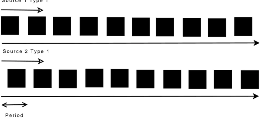
Figure 3.1 Audio ON-OFF Traffic Source Generator: x-axis is the time t, y-axis is the real amount of packets being sent divided by the maximum amount of packets possibly being generated if there is no OFF period between time 0 and time t . . . 65
Figure 3.2 Frame I Size Distribution: Generator Outputs (curve) and Trace File (histogram) . . . 69
Figure 3.3 Frame B Size Distribution: Generator Outputs (curve) and Trace File (histogram) . . . 70
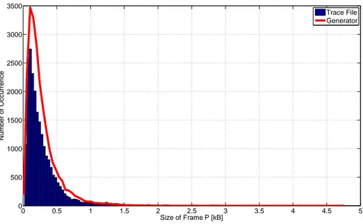
Figure 3.4 Frame P Size Distribution: Generator Outputs (curve) and Trace File (histogram) . . . 70 Figure 4.1 Admission Regions (Including Zero Lower Priority Traffic Source):
LiveTv-AF11 (StarWars IV MPEG-4 low quality) vs Data-AF41 (1480B Payload) for Different QoS under PQ . . . 74 Figure 4.2 Admission Regions: VoIP-EF (G.711, 160B Payload) vs
Data-AF41 (1480B Payload) for Different Queuing Disciplines . . . 75 Figure 4.3 Admission Regions: VoIP-EF (G.711, 160B Payload) vs
Audio-AF11 (G.711, 160B Payload) for Different PQ and RR . . . 78 Figure 4.4 Overall Loss Ratios for Both VoIP-EF and Data-AF41 by Adding
1Extra VoIP-EF Flow to the Curve WRR Weight 8:1 from Fig-ure 4.2 . . . 79 Figure 4.5 Admission Regions: LiveTv-AF11 (StarWars IV MPEG-4 low
quality) vs Data-AF41 (1480B Payload) for Different Queuing Disciplines . . . 81 Figure 4.6 Admission Regions: Command-AF11 (Command/Control
Sig-nals) vs Data-AF41 (1480B Payload) for Different Queuing Dis-ciplines . . . 82 Figure 5.1 Admission Regions: VoIP-EF (G.711, 160B Payload) vs
Data-AF41 (64Kbps) for Different CBR Data Packet Size . . . 86 Figure 5.2 Admission Regions: VoIP-EF (G.711, 160B Payload) vs
Data-AF41 (1480B Payload) for Different CBR Data Throughput . . 88 Figure 5.3 Admission Regions: VoIP-EF (G.711, 160B Payload) vs
Data-AF41 (64Kbps, 1480B Payload) for Different Server Capacity . 88 Figure 5.4 Admission Regions: LiveTV-AF11 (Star Wars IV Low Quality)
vs Data-AF41 (64Kbps) for Different CBR Data Packet Size . . 89 Figure 5.5 Admission Regions: LiveTV-AF11 (Star Wars IV) vs Data-AF41
(1480B) for Doubling Server Capacity and Data-AF41 Through-put) . . . 90
Figure 5.6 Admission Regions: LiveTV-AF11 (Star Wars IV) vs Data-AF41 (128Kbps) for Different Video Qualities, Server Capacity Be-comes 4Mbps . . . 91 Figure 5.7 Admission Regions: Command-AF11 (Command/Control
Sig-nals) vs Data-AF41 (64Kbps) for Different Data Packet Sizes . 92 Figure 5.8 Admission Regions: VoIP-EF (G.711, 160B Payload) vs
Audio-AF11 (G.711) for Different Audio-Audio-AF11 Payload Size . . . 93 Figure 5.9 Admission Regions: VoIP-EF (G.711) vs Audio-AF11 (G.711,
160B Payload) for Different VoIP-EF Payload Size . . . 94 Figure 5.10 Admission Regions: VoIP-EF (G.711) vs Audio-AF11 (G.711)
for Varying Both VoIP-EF and Audio-AF11 Payload Size . . . 95 Figure 5.11 Admission Regions: VoIP-EF (G.711, 160B Payload) vs
Audio-AF11 (G.711, 160B Payload) for Different Audio-Audio-AF11 Delay Service Level Agreement . . . 96 Figure 5.12 Admission Regions: VoIP-EF (G.711, 160B Payload) vs
LiveTV-AF11 (StarWars IV Low Quality) for Different LiveTV-LiveTV-AF11 Delay Service Level Agreement . . . 97 Figure 5.13 Admission Regions: VoIP-EF (G.711, 160B Payload) vs
LiveTV-AF11 (StarWars IV Low Quality) for Different LiveTV-LiveTV-AF11 Delay Service Level Agreement . . . 98 Figure 5.14 Admission Regions: LiveTV-EF (StarWars IV Low Quality) vs
Audio-AF11 (G.711, 160B Payload) . . . 99 Figure 6.1 Loss due to Delay of Audio-AF41 (low priority) . . . 104 Figure 6.2 Loss due to Delay of Audio-AF41 (low priority) . . . 104 Figure 7.1 Linear Approximation for the Admission Region: LiveTV-AF11
(StarWars IV MPEG-4 low quality) vs Data-AF41 (64Kbps, 1480B Payload) under PQ . . . 108 Figure 7.2 Linear Approximation for the Admission Region: VoIP-EF (G.711,
Figure 7.3 Linear Approximation for the Admission Region: VoIP-EF (G.711, 160B Payload) vs Data-AF4 (64Kbps, 1480B Payload) under WRR (8:1 Weight Ratio) . . . 109 Figure 7.4 Trapeze Approximation for the Admission Region: VoIP-EF (G.711,
160B Payload) vs Data-AF4 (64Kbps, 1480B Payload) under PQ 110 Figure 7.5 Step Approximation for the Admission Region: VoIP-EF (G.711,
160B Payload) vs Data-AF4 (64Kbps, 1480B Payload) under WRR (8:1 Weight Ratio) . . . 111 Figure 8.1 Admission Regions: VoIP-EF (G.711, 160B Payload) vs
Data-AF41 (1480B Payload) vs LiveTV-AF11 (StarWars IV Low Qual-ity) under Priority Queuing . . . 113 Figure 8.2 Admission Regions: VoIP-EF (G.711, 160B Payload) vs
Data-AF41 (1480B Payload) for Different Number of LiveTV-AF11 Traffics under Priority Queuing . . . 113 Figure 8.3 Admission Regions: VoIP-EF (G.711, 160B Payload) vs
LiveTV-AF11 (StarWars IV Low Quality) for Different Number of Data-AF41 Traffics under Priority Queuing . . . 114 Figure 8.4 Admission Regions: VoIP-EF (G.711, 160B Payload) vs
Data-AF41 (1480B Payload) for Different Number of LiveTV-AF11 Traffics under WRR (weight ratio 4 : 2 : 1) . . . 116
LIST OF NOTATIONS AND SYMBOLS
AC: Admission Control AR: Admission Region
AT M: Asynchronous Transfer Module
C: Line Capacity
CAC: Connection Admission Control CBR: Constant Bit Rate
Dif f Serv: Differential Service EB: Effective Bandwidth F IF O: First-In-First-Out F IF S: First-In-First-Serve F Q: Fair Queuing GOS: Group of Pictures
GP S: Generalized Processor Sharing h: Bin Width for an Histogram HT T P: Hypertext Transfer Protocol
IEEE: Institute of Electrical and Electronics Engineers IEF T: Internet Engineering Task Force
IP: Internet Protocol
IP DV: Internet Packet Delay Variation ISP: Internet Service Provider
IT U: International Telecommunication Union
IT U-T : Telecommunication Standardization Sector from ITU LIF O: Last-In-First-Out
LiveT V: Live Television
M P EG: Motion Picture Experts Group pdf: Probability Density Function P DV: Packet Delay Variation
P Q: Priority Queuing QoS: Quality of Service N aN: Not a Number RBD: Rate-Based Drop RF C: Requests for Comment
RR: Round Robin
s: Space
SIP: Signal Initiation Protocol SLA: Service Level Agreement
t: Time
T T L: Time to Live
V T C: Virtual Time Concept V oIP: Voice over IP
V oD: Video on Demand V O: Video Object V OP: Video Object Plane
W IRR: Weighted Interleaving Round Robin W RR: Weighted Round Robin
α(s, t): See EB
λ: Packet Arrival Rate µ: Packet Service Rate
LIST OF TABLES
Table 1.1 DSCP for AF PHB . . . 20 Table 1.2 Example of QoS Control Factors for Some Traffic Sources . . . 26 Table 3.1 Example of QoS Control Factors for Some Traffic Sources
(Ap-plications) . . . 57 Table 3.2 Size and Variance of Frames I, B and P for Different Video
Traf-fic Sources (e.g., Size of Frame I = E(I), Variance of Frame I Size = VAR(I)) . . . 66 Table 5.1 Size of Frames I, B and P for Star Wars IV (e.g., Size of Frame I
INTRODUCTION
Nowadays, connection admission control (CAC) concept has been widely used in ATM Network. The concept of CAC has extended its usage to IEEE 802.11 Wireless Network and IP networks (IPv4 and lately IPv6), wherever the communication is connection ori-ented [1, 2]. The demand on the high Quality-of-Service (QoS) performance for real time applications is growing rapidly. In order to guarantee the QoS of those new applications, CAC mechanisms play an important role. For fast accept/reject decision making on new incoming traffic, the notion of admission region (AR) has been heavily used. Previous studies show that for networks without differential service (DiffServ), linear approxima-tion is sufficient to make admission control decisions. In this thesis, CAC is applied to differential service (DiffServ) IP networks in order to verify if the statement about linear approximation holds as well for these types of networks.
Objective and Solution
The objective of this thesis is to find the admission region for different types of traffic source operating under DiffServ IP networks, and study the QoS behavior of these traffic. Yet, although many studies have been done in CAC and DiffServ; very few publications have taken both of them into consideration.
In this thesis, we propose a statistical simulation approach to study the impact of Diff-Serv on CAC. From the simulation results, we will determine whether the admission region is linear or not, and whether a linear approximation exists or not. We will also study the shape of the admission regions and related inputs (e.g., properties of each traf-fic source and the network) and outputs (e.g., delay, jitter and loss of each traftraf-fic type) from the simulations, and try to learn the correlations between them.
This thesis is organized as follows. Chapter 1 clarifies some basic terminologies and concepts for CAC, DiffServ, QoS and some previous research.
Chapter 2 has a full description of the simulation model (CAC SIM queuing model). The structure section will list all the components of the model and their properties/abilities. Later, there will be a detailed description on the queuing process, followed by the differ-ent techniques used in the simulations to help getting more reliable results in less time. The end of the chapter presents some validations tests.
Chapter 3 illustrates all the traffic generators, along with some validation tests. There are mainly 2 parts. Part 1 discusses all types of traffic sources (applications). Part 2 discusses all the generators used to emulate these traffic sources.
Chapter 4 mainly shows how different queuing disciplines affect the admission region of different traffic sources. The binding factors (dominant QoS factor) play important rule on shaping the admission regions for different queuing disciplines. In general, the weighted round robin admission curve stays in between the priority queuing (PQ) curve and the round robin (RR) curve.
Chapter 5 illustrates how the traffic source properties (such as packet size) and QoS boundaries (such as upper bound of delay constraint) would affect the admission region under priority queuing. In general, looser QoS constraint, larger packet size, greater throughput and greater server capacity would result larger admission region size. Chapter 6 attempts to explain why does jitter behave differently from other QoS (results shown in chapter 5). In general, the queuing system acts as a jitter buffer, which would convert some jitter problem into extra delay. This would explain why sometimes having more traffic flows results in lower jitter and higher delay.
method is the linear approximation.
Chapter 8 shows some results with 3 different types of traffic source in a network. The resulting admission region would be in 3-D or 2-D projection.
Conclusion will list all the important results and explore some ideas that could be tested someday in the future.
Contributions
In this research, we can show that the admission control can be used in DiffServ network. We can also show that it is possible to be approximated by linear approximations in the admission region plot.
We also study how different traffic flow characteristics, QoS constraints, queuing pro-cesses would affect admission regions. We try to generalize some rules though the ob-servations. We learn that changes in binding factor change the slop in admission region; WRR (weighted round robin) curves are always between PQ (priority queuing) and RR (rounded robin) curves; PQ does not always have larger admission region size than RR size; zero higher priority traffic flow may trigger huge increase in lower priority admis-sion; most traffic flow characteristics are directly proportional to admission region size; switching priorities may affect admission region shape and size; jitter behaves different from other QoS criteria. From these findings, hope one day we can obtain an analytical solution.
CHAPTER 1
BACKGROUND
In order to complete the ultimate goal of finding the admission region of different traffic sources in differential service, some terminologies must be well defined. This chapter includes a brief description of Connection Admission Control (CAC) and Differential Service (DiffServ) in section 1.1 and 1.2, followed by a short explanation on Quality-of-Serivce (QoS) control. The end of the chapter presents some prior research.
1.1 Connection Admission Control (CAC)
Admission control is a network QoS procedure that consists on deciding whether or not accept a new incoming traffic at call level (establish a new call or drop the call). There are many levels: electromagnetic wave level, bit level, packet level, frame level, call level, application level, etc. At the call level, a new network application requires to establish a connection, which is well known as the connection admission control (CAC) in ATM and 802.11 networks [2]. However, CAC can be implemented where the transmission is connection oriented (e.g. ATM, TCP, etc.). Most of the time, it happens in between the edge and core nodes of a network.
In a connection oriented network, CAC allows a new application initiation only if current network status, including the new admission, can support the minimum QoS requirement for the application. Thus, CAC algorithm has to compute the QoS parameters for all session types before it can accept a new session. This is too hard and the notion of effective bandwidth is used instead (see the section 1.1.1). CAC makes the accept/reject decision based on the characteristics of the incoming traffic and the network bandwidth usage status at that moment.
For a configuration (or a set) (n1, n2, ...ni)being authorized, where ni is the number of type i traffic source, all types of traffic must satisfy their own specific QoS requirements. The main idea of CAC is to avoid a new incoming traffic causing the QoS of all current active applications from deteriorating, or worse becoming unacceptable. It is similar to integrated service (IntServ) idea, except IntServ using reservation of line capacity (or reserve a fixed/known bandwidth). In the case of CAC, it would have to estimate the Effective Bandwidth of a traffic source. Ideally, if a new incoming source requires an effective bandwidth greater than current available bandwidth, then this new incoming traffic should be rejected. However, the computation of effective bandwidth is too com-plicated. Thus, an approximation (linear approximation in this thesis) using Admission Region is used. Both Effective Bandwidth and Admission Region will be explained in the sections 1.1.1 and 1.1.2.
1.1.1 Effective Bandwidth (EB)
Network resource is expressed in terms of bandwidth. The effective bandwidth (EB) of an application (or a traffic source) is the bandwidth required in order to have a satisfac-tory QoS for that application.
Effective bandwidth of a source i (EBi) is defined based on 2 free parameters, which are space s and time scale t, both positive and finite. For the amount of work X[0, t] (in our case the size of new arrived packets of the arrival process in terms of bits or bytes) that arrives from a source in the interval of time [0, t], Kelly defined the effective bandwidth α(s, t)of a source into a mathematical form (characteristic function) [3]:
α(s, t) = 1
stlogE[e
sX[0,t]] (1.1)
effective bandwidth: time independence, α(s, t) = f(st), additivity and α(s, t) = g(E[X], V AR[X])+h(s), where f(·), g(·) and h(·) are just some functions, and E[X] and VAR[X] are the expected value and variance of X. The details can be found in Kelly’s notes on effective bandwidth [3].
The reason why introducing Kelly’s definition in this research is because of his 3rd prop-erty, additivity, which says: If X[0, t] = P
iXi[0, t], where Xi[0, t] are independent, then
α(s, t) =X i
αi(s, t) (1.2)
This shows the property of additivity from the effective bandwidth, which is very useful through out the research. Since different traffic sources are generated independently, the overall effective bandwidth would be the summation of effective bandwidths for all current active traffic sources.
In practice, EB of application type i can be approximated from the bandwidth capacity C of a server and the maximum allowable number Ni = N∗ (N∗ is the test value) of such application with required QoS. Eq.1.3 is the simpler version of effective bandwidth definition, which can be used in the simulations due to its simplicity.
EBi = C
Ni (1.3)
This Ni is the largest number of connections (flows) allowed within the QoS constraints (or boundaries).
1.1.2 Admission Region (AR)
Recall Ni as the maximum number of traffic type i allowed simultaneously on a shared transmission line with a bandwidth capacity C. If there are 2 traffic types, then an ad-mission region graph can be plotted, where the adad-mission region is the area under the curve. The curve is called admission region curve, which is connected through dots (n1, n2) = (n1, N2). n1 and n2 are the number of traffic flows of type 1 and 2 respec-tively. N2 is the maximum number of type 2 traffic flows allowed. N2 = f (n1) is a function of n1, where n1 can be varied from 0 to N1 (max value of n1). Any config-uration (dot) (n1, n2) appeared above that curve would be rejected due to failed QoS test. Any configuration under the curve are acceptable. The dots on the curve are also acceptable.
Due to limited amount of resources, normally the rule of thumb is that the more type 1 traffic flows is being accepted, the more type 2 traffic flows would be rejected, and vice versa. The idea continues with 3 or more types of traffic, but the admission region would be 3-D space instead of 2-D area. However, sometimes there are exceptions. For example, when jitter becomes the dominant (bending) factor, the rule of thumb may not hold. (See details in later result sections.)
From equation 1.3, we have
C = EBiNi (1.4)
Due to the 3rdeffective bandwidth property mentioned above, if more than one type of traffic is present, we obtain
C = X
i
T r a f f i c S o u r c e 1 T r a f f i c S o u r c e 2 B o u n d a r y C u r v e o f A d m i s s i o n R e g i o n L i n e a r A p p r o x i m a t i o n o f B o u n d a r y C u r v e A d m i s s i o n R e g i o n T y p i c a l O p e r a t i n g R e g i o n
Figure 1.1 Illustration of Admission Region
The admission connection must make decision really fast due the massive amount of traffic flows. Thus simple solutions (less complexity) would be preferred. The solution could be a look-up table (LUT) for the admission region, or better an equation (preferable linear approximation for simplicity) approximating the admission region at its most used area.
Figure 1.1 illustrates an admission region plot for 2 types of traffic. Traffic source 1 and 2 are n1and n2 respectively. The admission region is the area under the curve. Notice that there is often a typical operating region. Thus, even though the admission region curve is not always linear, a linear approximation can still be applied to that typical operating region.
1.2 Differential Service (DiffServ)
There are 2 common ways to guarantee networking services: integrated service (IntServ) and differential service (DiffServ). While integrated service uses resource reservation protocol (RSVP) described in RFC 2205 to reserve bandwidth for a connection, differ-ential service guarantees different traffic sources with different service level agreements [4].
T r a f f i c S o u r c e 1
T r a f f i c S o u r c e 2
T r a f f i c S o u r c e 3
S i n g l e Q u e u e
S e r v e r
Figure 1.2 Illustration of Single Queue System
The reason why implementing differential service is that some traffic sources require very high quality of service due to their real time application in nature, while some other traffic sources may have no need of such high quality. Moreover, some traffic sources may have greater restriction on one QoS criterion while having much looser constraints on other QoS criteria. DiffServ differentiates these types of traffic sources. It classifies them into different priorities. Higher priority traffic flows would have priority to access resources.
In single queue system, there is only one queue for all the packets, thus all the traffic flows passing through this queue. Differential service however has to be applied on a multi-queue system. In order to activate the queuing process in a multi-queue system, a queuing discipline along with its setting (queuing policies) must be defined. A multi-queue system without taking priorities into account can be seen as single FIFO multi-queue with the potential possibility to differentiate the QoS agreement for each application. Figure 1.3 illustrates the queuing process in a queuing system at packet level. Once a packet arrives, it will enter a queue corresponding to its class. Notice that each queue corresponds to a priority, but there could be many traffic classes having the same priority, thus corresponding to the same queue. If the buffer of a queue is full, this queue will block new incoming packets of the same class. Some dropping policies would even drop a percentage of packets before the buffer reaches its full capacity. If all queues share
T r a f f i c S o u r c e 1 T r a f f i c S o u r c e 2 T r a f f i c S o u r c e 3 Q u e u e 2 S e r v e r Q u e u e 1 Q u e u e 3
Figure 1.3 Illustration of Multi-Queue System
the same buffer and the overall buffer is full, the lower priority queue will begin to drop some packets.
In this research, we assume that the packet storage process is using fixed buffer size on each queue, i.e. every queue has its own predefined buffer size. Commonly, a higher priority queue has less buffer size than the buffer size of a lower priority queue. The queuing process is set to be FIFO in this research, which means first in, first served by a server.
A packet could be classified by differential service code point (DSCP) for its priority (see section 1.2.3). The queuing disciplines and the queuing policies will be discussed in section 1.2.1 and 1.2.2.
1.2.1 Queuing Disciplines
All queuing disciplines are modeled to approximate the generalized processor sharing (GPS) [5]. Ideally, a traffic flow is broken into tiny little pieces, like a fluid. Think about fluid model: Many heterogeneous liquids (type of traffic) passing through a pipe (queue)
T r a f f i c S o u r c e 1 T r a f f i c S o u r c e 2 T r a f f i c S o u r c e 3 Q u e u e S e r v e r T r a f f i c S o u r c e 4
Figure 1.4 Illustration of Fair Fluid Queuing Model
and getting out of a valve (server). At any instant, each type of liquid is using a fixed portion of pipe and water cock in terms of radius. GPS is based on Fair Fluid Model, which combines a number of incoming flows into one combined flow with a density of each type of packets according to the original ratio. It is not practical because in network the transmission is in terms of packet, which can never be divided into infinite small size. However in reality, a traffic flow can never be broken into infinite small pieces, and the server can never treat different traffic flows at exactly the same moment. Since GPS is an ideal queuing discipline in terms of fairness, which cannot be implemented in reality. However it can be seen as a model, in which all other disciplines are trying to approximate this model. In other words, how fair a queuing discipline can be really defendant on how well it approximates the GPS model. In order to judge the performance on the queuing discipline, there are criteria other than fairness, such as complexity. Before discussing other queuing disciplines, here is a situation with 4 types of traffic sources (each generates 1 traffic flow in the network). Thus, there are 4 flows, which are F 1, F 2, F 3 and F 4 with weight ratios of 4 : 2 : 1 : 1 i.e. 50%, 25%, 12.5% and 12.5% respectively. Normal standard FIFO single queue system will serve any packet
according to its arrival time, regardless its priority.
GPS assumes that each packet of each flow can be divided into infinite small data, and that a single server can serve different flows simultaneously. This means at any given time t1, all 4 flows are transmitting data at that exact moment, thus F 1 will use 50% of the total bandwidth and F 2, 25% of the bandwidth while F 3 and F 4 each is using 25%. However, if at another time t2, there is no more data of F 1 and F 2 left, then F 3 and F 4 each will use 50% of the total bandwidth.
This scenario is illustrated in fluid model diagram (figure 1.4), and it will be later used to describe the small differences between queuing disciplines, such as priority queuing, fair queuing, weighted round robin, etc.
1.2.1.1 Virtual Time Concept (VTC)
Since a server can only serve one packet at a time, GPS (generalized processor sharing) cannot be implemented in reality, and one must decide which packet to be served first. Ideally, the packet requiring less time (waiting time + service time) should be served first. Due to the uncertain waiting time, any predicted (computed) timing is called virtual timing. There are 2 virtual times: virtual starting time and virtual finishing time. There are 2 conventional formula for these 2 virtual time computations.
Here are the 2 equations for computing the virtual starting time S(k, i) and the virtual finishing time F (k, i) of the kthpacket in session i:
S(k, i) = max(F (k − 1, i), V (a(k, i))) (1.6)
Notice that the virtual finishing time is zero when there is no packet (F (0, i) = 0). For a(k, i)being the arrival time a packet, L(k, i) is the length of that packet.
V (t)is the virtual time function for that dV (t)/dt = 1/SoASSaT , where SoASSaT is sum of active sessions shares at time t [5, 6].
There are some new algorithms, such as the new virtual time function used by dubbed weighted fair queuing 2+ (WF2Q+):
V (t + T ) = max(V (t) + T, min(S(h(i, t), i)) (1.8)
where h(i, t) is the packet number of the first packet in sessions ithqueue at time t. Also WF2Q+ can guarantee delay bounds given a session that is constrained with a leaky bucket [5, 6].
In general, it is very hard to emulate GPS because of the complexity for computing virtual times. Similarly, all queuing disciplines from the fair queuing (FQ) family require computation of virtual time, thus it would be harder to implement than round robin (RR) family.
1.2.1.2 Priority Queuing (PQ)
Priority Queuing (PQ) is the primary choice of queuing discipline in this research. Re-call that previous research has applied CAC on networks without DiffServ, and in this thesis, we apply CAC on IP networks with DiffServ. For all queuing disciplines, the strict higher-priority-first PQ provides the largest contrast to simple FIFO queue net-work (without DiffServ). PQ does not offer any service to lower priority queue until the higher priority queue is empty. There could be many priorities. For instance, Cisco has a four-level prioritizing traffic model. The four levels are high, medium, normal and low.
[4]
Back to the previous GPS example, for F 1 being priority 1, F 2 being priority 2, F 3 and F 4both being priority 3, F 1 in queue 1 will be served first. F 2 in queue 2 will begin transmission only after all F 1 packets in queue 1 are being served. Similarly, F 3 and F 4in queue 3 will be served at last, and it is FIFO for any packets in queue 3, regardless the packet is from F 3 or F 4.
The advantage of this discipline is that higher priority or more urgent packets has less waiting time. This discipline is also one of the simplest queuing disciplines in terms of complexity. The disadvantage is that the lower priority packets may never have a chance from obtaining service if higher priority packets keep arriving, which means PQ is less in favor, if not, least in favor of fairness.
In implementation, when a higher priority queue is not empty, there is no need to take care of lower priority queues except checking if their buffers are full.
1.2.1.3 Fair Queuing (FQ)
Fair queue (FQ) treats all the classes equally, which means there is no priority involved in the queuing process. Any packet having earliest estimated finishing time would be served first regardless from which traffic source. From the same previous example, it is possible that F 1, F 2, F 3 and F 4 each take one turn until there is no more packet left, assuming all packets have equal size.
FQ is completely different from FIFO single queue system. Fair queuing is using the virtual time concept (VTC) to compute the virtual finishing (service) time of a packet. Recall the virtual time computation in section 1.2.1.1. The packet that has the earliest of virtual finishing time, serves first. In fair queuing each type of traffic source has the same weight. Thus it often results in rotation for serving one packet of each type of traffic at
a time. In single queue system, it is simply according to the arrival time of each packet regardless its type. Thus fair queuing has greater fairness.
Advantage is that all the packets from different classes will also have a chance to be served, so that the heavy load of one traffic type can only slow other types of traffic flow down to certain degree. The disadvantage is that some more urgent packets may need to wait a relatively long period of time. Moreover, a disadvantage of the whole fair queuing family (FQ, WFQ, WF2Q, etc.) is that they need to compute predicted time (using virtual time concept) based on parameters such as packet size, which leads to highly complicated computations. Hence, rounded robin family (RR, WRR, WIRR, etc.) has been used in our research.
1.2.1.4 Round Robin (RR)
Round Robin (RR) or Packet Based Round Robin (PBRR) has the similar idea as fair queuing, except it considers everything at packet level (i.e. ignore packet size differ-ences). Instead of computing virtual time(s), it serves one packet from each type of traffic at a time. If the packet size is fixed, it will end up with exactly the same result as fair queuing, with much less complexity in implementation. Again, from the same example, F 1, F 2, F 3 and F 4 transmissions will be equally turn based, regardless the packet sizes.
The advantage is that the complexity of modeling is very simple, and that RR provides fairness. The disadvantage is similar to fair queuing, some real time applications may need to be served at higher priority unless the network resource is so abundant, which is not happening today.
1.2.1.5 Weighted Round Robin (WRR)
Weighted round robin is the round robin version of weighted fair queuing. Comparing to RR, it simply add a weight to each queue (class of traffic). From the previous example, the weight ratios could be 4 : 2 : 1 : 1, but also could be 8 : 4 : 2 : 2 or any 4x : 2x : x : x as x being any natural number. If there are always waiting packets in every queue, the service order would be F 1, F 1, F 1, F 1, F 2, F 2, F 3, F 4.
The advantage is still the less amount of complexity. Another advantage is that WRR does act as IntServ in which it reserves a limited minimum amount of bandwidth for lower priority traffic flow regardless the amount of higher priority traffic flow. The dis-advantage is similar to Weighted Fair Queuing (WFQ), which is the gaps problem. There is a big gap between servicing two groups of higher priority packets. As the same ex-ample illustrated before, the ratio between F 1 and F 2 without considering other lower priority traffic flow is 2 : 1. However, the weight system is set to be 4 : 2. In which, 2 consecutive F 2 packets would be served after 4 consecutive F 1 packets, which is not a good approximation of GPS in terms of fairness. In many applications, especially hand-shaking communications, this will cause problem. This is why there are other modified versions of WRR, such as weighted interleaving round robin (WIRR).
In implementation, in addition to round robin program, it just requires to add a counter for each queue for its weight.
1.2.1.6 Weighted Interleaving Round Robin (WIRR)
Weighted interleaving round robin is very similar to WRR. The slight difference could be illustrated by the common scenario as previous example, if there are always waiting packets in every queue, the service order would be F 1, F 1, F 2, F 1, F 1, F 2, F 3, F 4. For a 2 priority network, if the weight for the higher and lower priority traffic flow is N and 1 respectively, there is no difference between WIRR and WRR.
The advantage is the slight better fairness comparing to WRR (may reduce the delay). For simplicity, the weight ratio is set to be N : 1 in this research.
1.2.1.7 Other Disciplines and Policies
There are many other queuing disciplines. Here is a list of them (there may be more which are not included): Deficit Round Robin (DRR) or Deficit Weighted Round Robin (DWRR), Elastic Round Robin (ERR), Shaped Round Robin (SRR), etc. RR family queuing disciplines. There are also many FQ family queuing disciplines such as WFQ, WF2Q, WF2Q+, SCFQ, SFQ, LLQ, etc., which are beyond the scope of this research.
1.2.2 Queuing Policies
Each queuing discipline may operate differently when some settings are changed. Here are some most important settings: service order, pre-emptive mode, dropping policy, buffering.
1.2.2.1 Service Order
There are many types of service orders, such as come-serve (FCFS) or first-in-first-out (FIFO), last-first-in-first-out (LIFO), user defined custom setting, etc. In this re-search, we only consider FIFO queues.
1.2.2.2 Pre-emptive Mode
Pre-emptive mode is a strictly high priority first execution policy. If a lower priority packet is being hold in service, (i.e. packet in transmission, while started uploading to a transmission line but not finished yet.) and a higher priority packet arrives at that
moment, the lower priority packet would be instantly dropped for granting service to that higher priority packet if pre-emptive mode is on. Because that lower priority packet would be considered as a loss, leaving pre-emptive mode on would introduce significant amount of packet losses to lower priority traffic flows. In this research, pre-emptive mode is always off. This may result slight higher delay for higher priority packets. In theory, under priority queuing, only if the higher priority traffic flow outnumbers the lower priority traffic flow and that the lower priority packet size is comparable (preferred to be much larger) to the size of higher priority packet, the lower priority traffic flow will then affect QoS of the higher priority traffic flow.
1.2.2.3 Packet-Drop Policy
There are many ways to drop packets when buffer (queue) is full, such as drop tail and rate-based drop (RBD). The simplest is drop tail. It drops the last incoming packet when buffer is full.
Rate-Based-Drop drops packets with a buffer status (empty/full). For example, when buffer is less than 50% full, there is no dropping. When buffer is between 50% and 75% full, there is a probability of dropping some packets to maintain the buffer free space level. When buffer is above 75% full, it will drop at a higher probability. When buffer is nearly full, it will definitely drop some packets [7].
In real life, since the memory space becomes less expensive, there would be no dropped packets most the time. That is why many researchers tends to use unlimited buffer size (or a very large buffer), which means packet losses are often caused by failing QoS test such as delay and jitter tests. Large buffer deviation is not same as infinite buffer, and in practice, infinite buffer may cause memory leakage problem due to computer memory capacity in some cases.
1.2.2.4 Buffering
Buffer size stands for queue buffer size. In this research, each queue that represents a priority for certain traffic classes has its own buffer. Moreover, the lower priority queue has a larger buffer size than a higher priority queue, so that it can reduce packet loss due to buffer limitation as a normal internet service provider (ISP) would do in real world.
1.2.3 Differential Service Code Point(DSCP)
In general, there are 3 types of forwarding in DiffServ: Expected Forwarding (EF), Assured Forwarding (AF) and Best Effort (BE). EF tries to guarantee as much QoS as possible; BE has no QoS guarantee; and AF falls in between. These forwarding are all per-hop-behaviors (PHB). This means for a highest priority packet passing through node 1(e.g., a router), yet this packet could be considered as medium priority in node 2. The old IPv4 Type of Service (TOS) byte (8-bits) in an IP header is replaced by the dif-ferential service field. The first 6 bits are called Difdif-ferential Service Codepoint (DSCP), and the last two bits are Currently Unused (CU) [8].
DSCP serves to classify different network traffic applications. Notice that 2 packets with different DSCP may have the same priority at a node due to per-hop-behavior. Based on the used 6 bits, DSCP can define 64 different distinguished types of network services. If all 8 bits are used, DSCP can define up to 256 TOS.
Codepoint for Expedited Forwarding (EF) PHB is 1011102 = 46, where PHB stands for per-hop-behavior [9].
For Assured Forwarding (AF), there are 4 different subclasses each having 3 different dropping precedence. Codepoints for AF subclasses are shown in table 1.1. Overall, there are 12 subclasses in AF. For AFXY , smaller X represents higher priority, while Y
Drop Precedence Low Medium High
Class 1 AF11 0010102 = 10 AF12 0011002 = 12 AF13 0011102 = 14
Class 2 AF21 0100102 = 18 AF22 0101002 = 20 AF23 0101102 = 22
Class 3 AF31 0110102 = 26 AF32 0111002 = 28 AF33 0111102 = 30
Class 4 AF41 1000102 = 34 AF42 1001002 = 36 AF43 1001102 = 38
Table 1.1 DSCP for AF PHB
value only affects the dropping process [10].
Codepoint for Best Effort (BF) PHB is 0000002 = 0, which is the default PHB [10].
1.3 Quality of Service Control
There are mainly two type of quality of service control: Quality of Service (QoS) and Quality of Experience (QoE) [11]. QoE is measured as how many customers are satisfied at the application level. QoS focuses more on some performance measurements such as delay, jitter, loss ratio, throughput, etc., which is more at lower level (e.g. packet, frame, session). In this research, mainly 3 QoS criteria are taking into account: delay, jitter and loss. In the following sections, there will be detailed descriptions on these QoS factors and the way of measuring them.
1.3.1 Delay
The End-to-End delay is defined as the time required for a packet to travel from the source of origin to its destination [12]. For simplicity in this research, only the main components of the delay are considered, e.g. propagation time is considered to be zero. In this research, the delay of a packet is the time accounted from the instant when the packet enters its corresponding queue until it is sent, which mainly includes the time waiting in the queue and the transmission time.
Different types of application have different degrees of demand about the maximum end-to-end delay. VoIP for example, low delay is really important for a high quality audio stream during real time conversation. Although company Avaya has proposed 80-100ms in order to provide better quality than cell phones years ago, the maximum delay people using today is between 150 − 200ms for a relatively good quality VoIP. ITU-T G.114 suggests for highly interactive networking tasks, the delay must be below < 150ms (although sometimes, below 100ms delay may still affect the performance), and this maximum delay would provide good service for most applications. (Highly interactive applications include VoIP, video conferencing, interactive data applications, etc.) Based on their simulations for delay below 500ms, they suggest > 400ms to be unacceptable. Thus there is a gray area in between 150ms and 400ms [13, 14]. In this research, the maximum delay for high quality VoIP is set to be 150ms. 400ms delay upper bound was also used for few low quality VoIP.
The delay value usually increases very fast as the number of traffic flow increases. Sim-ilarly, the loss from delay conversion also increases exponentially. The details will be described in chapter 2 validation section.
1.3.2 Jitter
The jitter is defined as the delay variation. More specifically, it is the difference between the delay of a packet and a referenced delay value. There are 2 definitions of jitter, thus 2 different ways to measure the jitter proposed by International Telecommunication Union - Telecommunication Standardization Sector (ITU-T) and the Internet Engineering Task Force (IETF) respectively.
1.3.2.1 Definition of Jitter from ITU-T
ITU-T names jitter as packet delay variation (PDV). It uses Delaymin as the reference value for delay variation. As Jitteri, Delayi, Delaymin stand for the jitter for packet i, the delay for packet i and the minimum delay value for the packets belonging to the same type of traffic respectively, then the following equation defines the ITU-T version of jitter [15, 16, 17].
Jitteri = |Delayi− Delaymin| (1.9)
The implementation would be easy if the Delayminvalue is known in advance. However it is not in our case, where there is no way of telling how well the estimation of the Delaymincould be for some types of traffic (e.g. video traffic source).
Notice that sometimes the difference between Delayi and the reference delay value (in this case Delaymin) may be negative. Most researchers use absolute values for the jitter computation in order to avoid the trouble with the positive/negative signs.
1.3.2.2 Definition of Jitter from IETF
IETF, on the other hand, recommends using the previous packet delay as the reference value. In IETF, jitter is called IP delay variation (IPDV), except in RFC 3550, where the name jitter was introduced. Jitteri, Delayi, Delayi−1stand for jitter of packet i, delay of packet i and delay of packet i − 1, respectively. Then the following equation defines the IETF version of jitter [12, 18, 19].
The IETF version of jitter is easier to implement because there is no need to know any mean/min/max values in advance. However, if a packet has been lost or duplicated between the time that the packet has been sent and the time that packet has been received or not, there could be situations where Jitteri is infinite or become undefined. If the packet does not arrive to its destination within a reasonable time, its delay and jitter would also be considered undefined. RFC 3393 recommends to throw out these invalid samples in order to proceed any statistical collection process and analysis [18].
Hence, in this research, we have applied the IETF version of jitter. Moreover, each time Jitteri is being computed, while packet i may not arrive destination, packet i − 1 must be the previous packet of the same traffic type that has reached its destination. In other words, the reference delay value would be Delayi−2if packet i − 1 failed any QoS criterion and was considered as a loss.
If a network application requires high QoS in terms of jitter performance (e.g., less than 1ms), most often there would be a jitter buffer to decrease the variation of delay, which is jitter, by increasing average delay. Any new arrival packets would first pass through jitter buffer (a simple FIFO queue). These packets would exit the jitter buffer in a constant rate if there is always some packets in the buffer. The size of the jitter buffer is in terms of average waiting time in the buffer.
The final jitter measured from the output of a jitter buffer would mostly depend on the jitter buffer size instead of the original jitter. Larger jitter buffer size would cover greater jitter, but also increase the average delay. In general, the larger jitter buffer size, the better jitter QoS, as long as the new average delay would not exceed delay boundary. For the buffer size, some researchers use 60ms [20]. A typical jitter buffer size is 30ms ∼ 50ms, maximum 100ms ∼ 200ms for VoIP. However, over 100ms jitter buffer would cause more problem on the delay side. For high quality video traffic source, jitter below 20ms is excellent, and above 50ms is unacceptable. Cisco suggests 30ms for both audio and video traffic source [21].