A RESEARCH PROJECT TO STUDY PATTERNS, ROLES AND DETERMINANTS OF WOOD-DEPENDENT SPECIES DIVERSITY IN BELGIAN DECIDUOUS FORESTS (XYLOBIOS)

(1)

BELGIAN SCIENCE POLICY

HEAD OF THE DEPARTMENT ‘RESEARCH PROGRAMMES’: NICOLE HENRY (UNTIL SEPTEMBER 2007) DIRECTOR OF ‘RESEARCH AND APPLICATIONS’: DOMINIQUE FONTEYN (FROM APRIL 2006) CONTACT PERSON: ALINE VAN DER WERF

SPSD II (2000-2005)

FOR MORE GENERAL INFORMATION: SECRETARIAT: VÉRONIQUE MICHIELS WETENSCHAPSSTRAAT 8, RUE DE LA SCIENCE B-1000 BRUSSELS TEL : +32 (0)2 238 36 13

S P S D I I

A R E S E A R C H P R O J E C T T O S T U D Y PAT T E R N S ,

R O L E S A N D D E T E R M I N A N T S O F

W O O D - D E P E N D E N T S P E C I E S D I V E R S I T Y I N

B E L G I A N D E C I D U O U S F O R E S T S ( X Y L O B I O S )

M . D U F R Ê N E , J. R O N D E U X , P. G R O OTA E RT, P. L E B R U N PART 2 G L O B A L C H A N G E , E C O S Y S T E M S A N D B I O D I V E R S I T Y AT M O S P H E R E A N D C L I M AT E M A R I N E E C O S Y S T E M S A N D B I O D I V E R S I T Y T E R R E S T R I A L E C O S Y S T E M S A N D B I O D I V E R S I T Y N O RT H S E A A N TA R C T I C A B I O D I V E R S I T Y SPSD II A RESEARCH PROJECT T O STUD Y P A

TTERNS, ROLES AND DETERMINANTS

(2)

Part 2:

Global change, Ecosystems and Biodiversity

2001-2005

Marc Dufrêne (CRNFB) Patrick Grootaert (KBIN)

Philippe Lebrun (UCL) Jacques Rondeux (FUSAGx)

Main text

Written by Philippe Fayt (CRNFB), except for the Chapters 5 (Jean-Marc Henin, FUSAGx) and 6 (Philippe Lejeune, FUSAGx)

December 2006

(SPSDII)

FINAL REPORT

A RESEARCH PROJECT TO STUDY PATTERNS, ROLES AND DETERMINANTS OF WOOD-DEPENDENT SPECIES DIVERSITY

IN BELGIAN DECIDUOUS FORESTS (XYLOBIOS)

(3)

D/2008/1191/10

Published in 2007 by the Belgian Science Policy Rue de la Science 8 Wetenschapsstraat 8 B-1000 Brussels Belgium Tel: + 32 (0)2 238 34 11 – Fax: + 32 (0)2 230 59 12 http://www.belspo.be Contact person:

Mrs Aline Van der Werf

Secretariat: + 32 (0)2 238 36 13

Neither the Belgian Science Policy nor any person acting on behalf of the Belgian Science Policy is responsible for the use which might be made of the following information. The authors are responsible for the content.

No part of this publication may be reproduced, stored in a retrieval system, or transmitted in any form or by any means, electronic, mechanical, photocopying, recording, or otherwise, without indicating the reference.

(4)

in Belgian deciduous forests (XYLOBIOS) »

Core research team

Philippe Fayt1*, Marc Dufrêne1*, Etienne Branquart1*, David Dufour2, Pierre Hastir3, Jean-Marc Henin2, Philippe Lejeune2, Jonathan Lhoir3, Christophe Pontégnie3, Ben Van Der Wijden4, Sven Verkem4, Veerle Versteirt5 and Ruben Walleyn6

1_{Research Centre of Nature, Forests and Wood (CRNFB), Av. Maréchal Juin 23, B-5030 Gembloux,} 2_{Forest and Nature Management Unit, Gembloux Agricultural University (FUSAGx), Passage des}

Déportés 2, B-5030 Gembloux, 3_{Biodiversity Research Centre, Catholic University of Louvain (UCL),}

Croix du sud 4-5, B-1348 Louvain-La-Neuve, 4A.B.Consultancy g.c.v., Cyriel Buyssestraat 88, B-2020 Antwerpen, 5Department of Entomology, Royal Belgian Institute of Natural Sciences (IRSNB), Vautierstraat 29, B-1000 Brussels, 6Research Institute for Nature and Forest (INBO), Gaverstraat 4, B-9500 Geraardsbergen

*Project coordinators

User committee

CEMAGREF (Institut de recherche pour l'ingénierie de l'agriculture et de l'environnement)

DNF (Division de la Nature et des Forêts, Ministère de la Région wallonne) Forêt Wallonne asbl

IDF (Institut pour le développement forestier)

INBO (Research Institute for Nature and Forest (Flemish Government, formerly IBW – Institute for Forestry and Game Management)

(5)

(6)

ACKNOWLEDGMENTS

This final report presents the major results of activities carried out in the framework of the XYLOBIOS project (n° EV/H1/15A) from 2001-2005. It benefited from the commune contribution of the Research Centre of Nature, Forests and Wood of the

Ministry of the Walloon region (CRNFB, DGRNE), the Forest and Nature

Management Unit of the Gembloux Agricultural University (FSAGx), the Biodiversity Research Centre of the Catholic University of Louvain (UCL), and the Department of Entomology of the Royal Belgian Institute of Natural Sciences (IRSNB), under the supervision of the CRNFB.

Moreover, such a multidisciplinary and challenging project required the expertise from many specialists to be put together. The project greatly benefited from the help of Ruben Walleyn (INBO) who carried extensive inventories of wood-decaying fungi in our study sites. Also, David Dufour (FUSAGx) is acknowledged for bird monitoring at early hours as well as Agnès Guerin (FUSAGx), Bart Christiaens and Peter Van de Kerckhove (INBO) for their sustained effort in soil sampling. Ben Van Der Wijden and Sven Verkem (A.B.Consultancy g.c.v.), after having spent countless hours under difficult monitoring conditions, provided us with new insights into bat ecology and distribution in southern Belgium. Additionally, one should especially acknowledge Jean-Yves Baugnée, Pierre Hastir, Jonathan Lhoir and Marc Mignon for their main contribution in insect searching, sorting, identifying and plant monitoring. Laurent Dombret, Arnaud Gotanegre and Céline Prévot are thanked for their help in insect sorting. Stéphane Pierre is greatly acknowledged for efficient contribution in scolytid identification, and Lucien Leseigneur and Benoit Dodelin for their help in the identification of a not so typical eucnemid species. Dr. Patrick Grootaert and the technicians of the Royal Belgian Institute of Natural sciences are appreciated for their (technical) support.

Among other contributors, the Xylobios research team would like to thank particularly Roger Dajoz, Philippe Lebrun, Petri Martikainen, Louis-Michel Nageleisen and Martin C.D. Speight for their precious pieces of advice on insect sampling at the early stage of the project.

Finally, the researchers involved in the project wish to express their gratitude to collaborators from the “Division de la Nature et des Forêts” and “AMINAL / Afdeling Bos en Groen” for having provided information and access to the different study sites.

(7)

TABLE OF CONTENTS

ABSTRACT ... 9

1. INTRODUCTION ... 11

2. SAMPLING SAPROXYLIC DIVERSITY (WP1) ... 15

2.1. Studying saproxylic organisms in Belgium: why, which and where? ... 15

2.2. Sampling wood-dependent organisms: how? ... 16

2.2.1. Insects ... 16

2.2.2. Wood-decaying fungi... 18

2.2.3. Forest birds... 19

2.2.4. Bats... 20

2.3. How efficient is the sampling? Saproxylic insects as an example ... 21

3. UNDERSTANDING WOOD-DEPENDENT BIODIVERSITY (WP2) ... 25

3.1. Site characteristics ... 25

3.2. Sampling scheme... 28

3.3. Factors explaining species number and abundance... 29

3.3.1. Insects ... 29

3.3.2. Wood-decaying fungi... 43

3.3.3. Forest birds... 44

3.3.4. Bats... 47

4. WOODY DEBRIS, NUTRIENT CYCLING AND SOIL FERTILITY (WP3)... 49

4.1. Influence of overall dead wood supply on stand soil fertility ... 50

4.1.1. Material and methods ... 50

4.1.2. Results... 50

4.2. Influence of decaying log proximity and history on soil fertility ... 53

4.2.1. Material and methods ... 53

4.2.2. Results... 53

5. UNDERSTANDING TREE MORTALITY: THE CASE OF THE “WALLOON BEECH DISEASE” (WP5)... 57

5.1. Development of the “beech disease”: short summary ... 59

5.2. Epidemiology of the disease: hypotheses and explanations ... 60

5.2.1. Attacks of 1999 and 2000... 60

5.2.2. Trypodendron spp. population dynamics ... 61

5.2.3. Attacks of 2001... 67

5.2.4. The role of fungi... 69

5.3. Aggravating elements ... 70

5.4. Role of dead wood and saproxylic organisms in the beech disease ... 72

(8)

6. MODELLING DEAD WOOD AND LEGACY TREE RETENTION IN RELATION TO VARIOUS FOREST MANAGEMENT PLANS, WITH IMPLICATIONS FOR FOREST PRODUCTION

LOSS (WP6) ... 77

6.1. Simulation of CWD and LT retention... 77

6.1.1. Introduction ... 77

6.1.2. Growth model ... 78

6.1.3. Mortality of trees and designation of legacy trees... 78

6.1.4. Decay process of CWD ... 79

6.1.5. Presentation of the model... 79

6.2. Impact of CWD and LT retention on productivity loss... 80

6.3. Application of the simulation model... 80

6.3.1. Introduction ... 80

6.3.2. Initial stand and model parameters ... 83

6.3.3. Results... 83

6.3.4. Analysis of the sensitivity of the model... 84

6.4. Conclusion and recommendation... 84

7. GENERAL DISCUSSION... 87

7.1. The context of the research ... 87

7.2. Ecological and functional benefits of dead wood: a brief summary ... 89

7.3. Implications of the results for biodiversity and forest management ... 90

7.4. Conclusions... 97

REFERENCES ... 99

PUBLICATIONS, POSTERS AND COMMUNICATIONS... 115

(9)

(10)

ABSTRACT

Key-words: Belgium, biodiversity, dead wood, deciduous forest, saproxylic

Originating from the cautious recommendations by the European Council and the Bern Convention to retard the current erosion of biodiversity and link species loss with ecosystem functioning, this project aimed to clarify the ecological and functional values of dead wood habitats (including dead parts of living trees) in Belgian oak and beech forests. Among ecological benefits, we were interested to assess the relative importance of dead woody debris for representative species groups of forest biodiversity such as saproxylic insects, wood-decaying macrofungi, cavity-nesting birds and bats. At times when numerous beech trees were dying over a large part of southern Belgium, we wanted to see whether the development of large populations of damaging beetles in individual stands was causally related to a high dead wood supply, or if perhaps other factors would also come into picture. Among benefits for forest functioning, the possibility that a high supply of decaying wood on the forest floor could influence the geochemistry of the soil upper layer, with implications for plant growth and stand productivity, needed some clarification. From a management perspective, retaining overmature and dead trees for biodiversity implies some loss of production for the forest owner, which should be estimated when trying to optimise wood production at minimal costs.

We found the amount of dead wood to be highly beneficial for saproxylic insect, macrofungi and bird species diversity. Among insects, bark beetles, including the potentially damaging ambrosia beetles (Trypodendron spp.), were more numerous in stands classified as with dead wood (55 m3 ha-1 on average) than stands without dead wood (12 m3 ha-1 on average). However, they were not more numerous in those stands with a dead wood volume above 50 m3 ha-1 compared to those with a lower dead wood supply. Besides a better understanding of key ecological factors for the different taxa, perhaps a major finding of our research was the confirmation of critical thresholds for those different factors below which risks of population depletion and species extinction are greatly increased. By providing threshold values for diverse habitat parameters shown to be important for numerous saproxylic species, this project calls for forest management procedures that also take into account their biological requirements in the management plans. Furthermore, the retention of those key habitats for biodiversity does not contradict with wood production for economical purposes, as shown for example by our estimates of soil fertility or bark beetle population size at the highest dead wood volume.

(11)

(12)

1. INTRODUCTION

Dead wood is a conspicuous and multifunctional component of dynamic forest ecosystems. Under natural conditions, its accumulation in a stand is determined by the balance between input and decay rates (Siitonen 2001). The input rate is related to the stand successional stage. As the stand develops, the amount of woody debris produced by annual mortality increases, first due to competition and self-thinning, and later because of older trees becoming more susceptible to disturbance factors such as wind, insects and disease (Harmon et al. 1986). Prevailing disturbance regime and site productivity affect the volume of dead wood as well (Sturtevant et al. 1997). The decay rate of woody debris, on the other hand, is a function of tree species, tree size, wood quality, and climate, which control the activity of decomposing organisms (Morrison & Raphael 1993, Siitonen 2001).

Recent inventories of naturally dynamic forests have revealed dead wood volumes between 40 to 200 m3 ha-1 (Vallauri et al. 2002), sometimes up to 570 m3ha-1 (Christensen et al. 2005), depending on the regions and dominant tree composition. The proportion of snags and logs of the dead wood volume vary considerably between vegetation types, with different tree species having different modes of death. In the natural forests of Northern Europe, snags are typically more numerous in Scots pine Pinus sylvestris dominated stands compared to spruce Picea abies dominated forests, due to a higher susceptibility of spruce trees to uprooting and stem breakage (Liu & Hytteborn 1991, Siitonen et al. 2000). Similarly, in temperate deciduous forests, old beech trees Fagus sylvatica become increasingly predisposed to break-up compared to oak Quercus spp, with implications for gap dynamics (Mountford 2004). On average, it is usual to find between 40 to 140 snags, 10-40 broken stems, and 10-20 (up to 60) cavity trees per hectare of broad-leaved old-growth forests (Vallauri et al. 2002). In the Bialowieza primeval forest, Poland, dead wood accounts on average for 5-30% of the standing wood volume (Falinski 1978). During the last decades saproxylic organisms, those that depend upon wood substrates or upon the presence of other saproxylics for at least part of their life cycle (Speight 1989), have received increasing attention from ecologists, conservation biologists, and forest managers (Samuelsson et al. 1994, Grove 2002, Vallauri et al. 2002). Detailed species inventories showed their highly significant contribution to forest overall species diversity. In Finland for example, a conservative estimate of 4000 to 5000 species has been suggested to depend on dead wood habitats, which account for as much as 20-25% of all forest-dwelling species (Siitonen 2001). In Germany, about 1500 species of fungi and about 1350 species of beetles, major contributors to the earth biodiversity (Franklin 1993), are known to live exclusively on

(13)

dead wood (Albrecht 1991). In Norway and in Sweden, approximately 1000 saproxylic beetles have been inventoried (Økland et al. 1996, Jonsell et al. 1998). Wood-dependent organisms are also functionally important to forest ecosystems. They play critical roles during the processes of woody debris decomposition and nutrient cycling through multitrophic interactions (Harmon et al. 1986, 1994, Edmonds & Eglitis 1989, Bengtsson et al. 1997). By contributing to natural tree mortality, they influence forest structure and composition (Kuuluvainen 2002). The availability of saproxylic insects affects forest bird communities, notably by limiting the populations of most woodpecker species, important cavity providers for secondary cavity-nesters (Martin & Eadie 1999, Bednarz et al. 2004).

Some saproxylic organisms have narrow micro-habitat requirements and poor dispersal capacities (Siitonen 2001, Grove 2002). This makes them a group of species particularly susceptible to habitat loss and fragmentation and, as a result, extinction-prone. Accordingly, Speight (1989) estimated some 40% of Europe’s saproxylic invertebrates to be already on the verge of extinction over much of their range while the majority of the remainder would be in decline. Due to their specificity for substrate and microclimatic conditions characterising mature timber habitat, saproxylic communities have been suggested as useful bio-indicators of forest quality, and as tools in the process of identifying important forests for nature conservation (Speight 1989, Good & Speight 1996). Ultimately, a major argument for maintaining dead wood habitats and preserving saproxylic assemblages is that losses of saproxylic species diversity may impair processes required for the long-term functioning of the forest ecosystems (Bengtsson et al. 2000), such as nutrient cycling.

An important reason why woody debris are systematically removed from forests originate from the specificity of a very few among saproxylic insects (less than 1% of all forest insect species (Nageleisen 2003)), mainly bark beetles (Coleoptera, Scolytidae), to reach under particular environmental conditions epidemic levels and kill apparently healthy trees in large numbers (Vité 1989). Fear of significant economical losses has even led authorities to establish in some countries regulations for forest protection from so-called insect pests (Ehnström 2001). Cautious management procedures stem mostly from widespread observations that stand hazard and windthrown trees act as major factors determining risk of beetle outbreak (e.g., Reynolds & Holsten 1994). On the other hand, contrarily to the common belief that forest management helps to limit bark beetle populations, studies comparing saproxylic assemblages between managed and natural forests have brought surprising results. Already in 1968, Nuorteva remarked that the thinning and clear-cutting of finnish forests lead to the increase of bark beetle population, presumably as a result of increased availability of breeding material and warmer temperature

(14)

conditions. Still in Finland, looking at the trunk fauna of coniferous trees, Väisänen et al. (1993) found the proportion of bark beetles to be about 52% of the individual beetles collected in managed forests, but only 3% in natural old-growth forests. This was recently confirmed by Martikainen et al. (2000), who found the proportion of bark beetles out of all saproxylic beetles caught smaller in old-growth than in managed forests, despite roughly five to tenfold more decaying wood in the former habitat. In similar old-growth habitats, Fayt (2003a,b) found primary conifer bark beetles to account for only 1.14% of the total catch (25,000 bark beetles). The same pattern holds whether the insects were collected with standard window-flight traps or from bark samples. In German commercial forest where dying and dead trees have been retained for a decade, bark beetle species known as pest species contributed to less than 10% of the number of all beetle individuals captured (Kleinevoss et al. 1996). Inversely, bark-beetle predators and other enemies (parasitoids) have been found more abundant in unmanaged forests, probably as a result of the higher amount and diversity of recently dead wood (Martikainen et al. 1999). Those findings suggest a possible role for wood-living predators and associates in regulating partly bark beetle populations below epidemic levels, as long as enough decaying wood is available. Although Europe covers a relatively small area of the globe, it is characterised by various kinds of forest landscapes, with management histories that are specific to a particular country (Mikusiński & Angelstam 1998). Spatial variation in composition and structural heterogeneity reflects the profound impacts that the past geopolitical location of the different countries has had on the amount of deforestation and intensity of landscape transformation. Already 2000 years ago, very few patches of secondary forests were left apart in the Mediterranean region (Speight 1989). In western Europe, roots of this phenomenon dates back in particular to the eighteenth and nineteenth centuries, when the start of the Industrial Revolution lead to dramatic economical developments in the United Kingdom before to spread towards other western European countries, with direct implications for forest uses. Simultaneously, large tracks of naturally dynamic forests remained little affected in the east or some parts of Fennoscandia and western Russia. As a result, the present-day European countries clearly differ in terms of the proportion of the forest land that has retained elements of the original forest cover, namely a high tree species diversity with a dominant deciduous component, a continuous supply of large overmature and dead trees, and on-going vegetation dynamics. Perhaps one of the most obvious consequence is a general impoverishment of the biological legacy of European forests from the east to the west, as shown for example for woodpecker species diversity (Mikusiński & Angelstam 1998).

With an area of 30,230 km2 and forests covering 22.2% of the land, Belgium is one of those western European countries that have undergone dramatic changes in forest

(15)

cover, composition and structure during the last centuries. As a general observation, use and transformation of Belgian forest landscapes has been closely connected to the changing economical needs of developing human societies (Tallier 1998). From a saproxylic organism’s point of view, living conditions have been profoundly deteriorated. In Wallonia, in the southern half of the country, Lecomte mentioned in 2006 an average dead wood volume of 6 (beech) and 7.5 (oak) m3 ha-1, based on the Walloon Permanent Forest Resource Inventory. This is particularly low if compared with volumes found under natural conditions (Vallauri et al. 2002), corresponding to a dead wood reduction over 95% (!). In addition to habitat loss, which is known to cause species extinction in a non-linear manner (Connor & McCoy 1979), the forest cover has been increasingly fragmented and relict saproxylic populations increasingly isolated, whether directly (e.g., agriculture, road network,…) or in a more subtle way (e.g., large-scale afforestation with non-native conifer trees). Depending on the region, populations of wood-dependant organisms are expected to have badly suffered from the loss of spatio-temporal continuity in suitable ecological conditions, with implications for species persistence (Nilsson & Baranowski 1997, Kehler & Bondrup-Nielsen 1999, Sippola & Renvall 1999, Nilsson et al. 2001).

In this report, we describe the objectives and the methods of the four-year research project named XYLOBIOS and we discuss its main results, mentioning implications for forest management. The project originates from the cautious recommendations of the European Council and the Bern Convention to retard the current dramatic erosion of biodiversity and link species loss with ecosystem functioning (Speight 1989, Good & Speight 1996). Its general aim is to address simultaneously and to link both major ecological and economical issues raised by the management of decaying woody debris in native mature deciduous forests (beech Fagus sylvatica and oak Quercus spp. dominated-) of central-southern Belgium. Notably, by providing new insights into key environmental factors for the distribution of saproxylic diversity, this project should help in the development of management guidelines favourable to biodiversity in temperate forests. Several Belgian research institutions took part in the project, among which two universities (FUSAGx, UCL), the Research Centre of Nature, Forests and Wood (DGRNE - Ministry of the Walloon region), and the Royal Belgian Institute of Natural Sciences (KBIN/IRSNB).

The report is subdivided into different work packages (WP), each with its own objectives, methods, results and possible implications for the research on saproxylic organisms in Belgium and their conservation in relation to diverse management scenarios. Basically, the project aimed to develop a national expertise in the study of distribution, diversity, ecology and roles of saproxylic organisms of deciduous forests.

(16)

2. SAMPLING SAPROXYLIC DIVERSITY (WP1)

2.1. Studying saproxylic organisms in Belgium: why, which and where?

Because of highly diverse and specialised requirements for woody substrates, limited dispersal abilities and their consequent sensitivity to habitat loss and fragmentation, part of saproxylic organisms have been suggested as potential useful bio-indicators of global forest quality (Speight 1989, Good & Speight 1996). One aspect covered by the project was to gain reliable and informative data on the current distribution of saproxylic organisms, aiding in the process of identifying important forests in Belgium for nature conservation. We were also particularly interested to clarify those environmental factors that best explained their local distribution, with emphasis on the effect of dead wood supply and quality on species diversity and abundance. Among practical implications, it was relevant to assess whether the accumulation of woody debris makes individual stands more susceptible to attacks by damaging beetles, with economical consequences, or not necessarily. Understanding species distribution, on the other hand, is a prerequisite in the process of correctly predicting priority habitats for forest biodiversity.

In this project, the selection of meaningful forest indicators followed Speight (1989)’s criteria, mainly that those species should (i) depend upon dead wood of dying and dead trees for their habitats, and (ii) be relatively easy to find and to determine. Information on their micro-habitat preferences and general life-history should also be available in ecological textbooks. We focused our research on four distinct taxonomic groups known for their preference for micro-habitats (woody debris, trunk cavities, rot-holes, …) and foraging grounds that typically develop in overmature stands, namely saproxylic insects, wood-decaying fungi, cavity-nesting birds, and bats. Among insects, we restricted the identification work to families for which we had taxonomic competence. We limited fungi monitoring to those species producing larger fruiting-bodies (macromycetes). Hole-nesting birds included both primary cavity nesters (i.e., excavators) and secondary cavity users (i.e., non-excavators), while non-cavity nesters were used as a control.

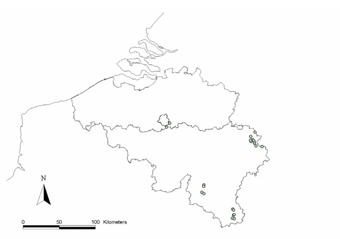
The selection of relevant study sites benefited from the help of the different forest districts, to whom we made enquiries about available forest statistics. Following field confirmation, a total of 22 sites (10 beech and 12 oak-dominated stands) were selected, distributed over four natural regions (Fig. 1). Dominant tree composition (oak/beech), forest age and availability of woody debris were the main criteria of selection.

(17)

Figure 1. Location of the study sites (circles).

Sites were organised by pair (11 pairs), with pair stands showing similar plant composition, soil properties and abiotic factors (elevation) but differing visually in their overall amount of coarse woody debris. Accordingly, paired-stands were thereafter classified as having a high (or with dead wood) vs. low dead wood supply (or without dead wood) (Appendix 1). They were located 2-10 km apart from each other.

2.2. Sampling wood-dependent organisms: how?

2.2.1. Insects

We used various kinds of traps to study the insect composition of the different study sites, based on their trapping efficiency from the literature. Among available capture devices, flight-interception traps have been shown to capture a significant part of the flying beetle fauna (Muona 1999, Similä 2002), including saproxylic species (Siitonen 1994, Økland et al. 1996, Martikainen et al. 2000, McIntosh et al. 2001). Two main variants of this trap model exist, either placed independently of woody substrates (flight-window traps) or attached to tree trunks (trunk-window traps, Kaila 1993). Flight-window traps are suitable for comparing different forest environments, but are related to ecological conditions over wide areas (Økland 1996). This means that the

(18)

position of the trap in relation to dead wood distribution does not greatly affect the number of species and individuals caught (Siitonen 1994). By contrast, trunk-window traps are more suitable for comparison of different substrates within the same forest environment than between forest stands (Kaila et al. 1994). This is because the substrate on which the trap is attached (typically trunks of dead trees, often close to the fruiting-bodies of polypores) serves as a bait, which has a strong effect on the composition of the species caught. Trunk-window traps are more effective in catching rare and threatened saproxylic species than freely-hanging flight-window traps (Martikainen 2000). Part of the insects (e.g., Diptera, Hymenoptera), however, have flying-abilities good enough to avoid obstacles, making them difficult to collect with conventional flight-interception traps. Instead, their propensity to avoid an obstacle by flying upwards towards the light makes them more susceptible to capture by Malaise traps (Malaise 1937). Finally, emergence traps allow the capture of insects when emerging from their breeding habitats, providing information on larval micro-habitat preferences (Owen 1989).

We sampled insects from March to October 2002-2003. The applied sampling protocol aimed to maximise sampling efficiency (i.e., collecting enough individual species to approach the true community value) of the target groups, while allowing comparison between sites (Fig. 2). In the 11 sites with a high amount of dead wood, insect traps were situated where woody debris were most abundant. In each stand, 8 flight-window traps (W) were placed and numbered along 2 x 100 m perpendicular transects crossing each other in their middle, with the traps number 1, 2, 3, 4 in the north-south direction, and the traps 5, 6, 7, 8 in the west-east direction. Traps 1-2, 3-4 and 5-6, 7-8 were suspended on a metal wire between trees 25 m apart, leaving the transect junction (between traps 2-3 and 6-7) free of window traps. Flight-window traps consisted of two perpendicular intercepting 40 x 60 cm transparent plastic panels, with a funnel leading to a container below the panels filled with water, salt and detergent. Traps were covered with a transparent 80 x 80 cm plastic roof to minimise funnel obstruction with plant debris and to divert rainfall. In those 11 stands with high dead wood volume, we added 8 roof-covered trunk-window traps of 2 x 40 x 60 cm (K); they were attached to randomly selected standing dead trees, with 2 traps per quarter of the sample plot. Contrarily to flight-window traps, funnels used for trunk-window traps were made flexible to facilitate a closer contact of the window against the trunk. To optimise the capture of insects that have contrasting flight behaviour and host preferences, we also used 2 Malaise (M) and 3 stump-emergence (E) traps. Malaise tents (with a second one only in 2003) were located apart near the centre of the plot in a sunny place, with ethylene-glycol in the container to preserve the insects. They were protected from wild boars Sus scrofa by a robust metal fence stretched on wooden posts. In 2003, together with the second

(19)

Malaise trap, we placed 1 intercept panel trap® (PS), made of black cardboard panels, where the sampling transects crossed.

Figure 2. Schematic view of a sampling unit designed to monitor local saproxylic insect diversity. Letters W, K, M, E refer to the different kinds of trap under use (see text for details). Traps were emptied once a month and regular visits were made in May-June to minimise the risks of trap funnel obstruction at times of maximum insect activity.

2.2.2. Wood-decaying fungi

Wood-inhabiting fungi account for a high proportion of known forest species. Only in Finland, they would represent up to 30-40% of the saproxylic species (Siitonen 2001). Key actors in the process of wood decomposition, fungi also influence the diversity of other organisms associated with dead wood, e.g. saproxylic insects (Jonsell & Nordlander 2002, Komonen 2003).

A survey of wood-inhabiting macrofungi was carried out by Ruben Walleyn (INBO) in 10 selected beech stands (5 pairs). Special attention was paid to strictly lignicolous macrofungi: agaricoid and boletoid fungi, gasteromycetes, hydnoid fungi, polypores, major corticioid fungi (Chondrostereum, Cristinia, Cystostereum, Laxitextum, Mycoacia, Phlebia, Peniophora, Steccherinum, Stereum), heterobasidiomycetes with

(20)

fruitbodies larger then 1 cm, discomycetes with fruit bodies > 1 cm, and larger Pyrenomycetes: Camarops, Eutypa and Xylariaceae. The species inventory was based on the presence of fruiting bodies within a 4 ha sample plot, centred on the circular insect sample plot delimited by perpendicular transects. It took place in autumn-winter 2002-2004, each site being visited 2-5 times, depending on the amount of dead wood available (i.e., census effort) (Walleyn et al. 2004).

2.2.3. Forest birds

As a general pattern, cavity nesting bird density, diversity, and species richness are strongly positively influenced by increases in stand age and average tree dbh (diameter at breast height) (Ferry & Frochot 1970, Land et al. 1989, Newton 1994), as long as dead trees are not systematically removed. Among cavity users, primary cavity nesters (i.e., excavators such as woodpeckers) are keystone species in the forest environment, influencing the composition and abundance of obligate and facultative hole-nesting vertebrate communities (Martin & Eadie 1999; Bednarz et al. 2004, Martin et al. 2004). In Europe, about half of forest bird species use tree cavities for reproduction and maintenance activities.

In 2003, David Dufour (FUSAGx) estimated forest bird species and individual numbers among 16 of the 22 stands, located in eastern (Hertogenwald) and southernmost Belgium (Lorraine). Stands were organised by pairs (8), with half of them being classified as with a high volume of woody debris. Bird inventory was carried out from February-June 2003 in early morning (from dawn till 10 a.m.) under mild weather conditions (limited wind and no rainfall). Individual birds were censused by point counts, that is counts undertaken from a fixed location for a fixed time period (Gibbons et al. 1996). This method was preferred instead of other existing sampling alternatives such as territory mapping or presence/absence (EFP, Grimoldi 1976), providing estimates of the relative abundance of each species between habitats with limited effort (Muller 1987).

Except for woodpeckers, point count stations (the position from which the count was made) were laid out in a systematic manner within the study plots, with 3 point counts/site in homogeneous habitat conditions. To avoid counting the same individuals, count stations were selected to have a minimum distance of 300 m between each other. They were centred on the circular insect sample plot. The survey was splitted into two periods over the spring, to ensure the counting of early (mostly sedentary species) and late singers (i.e., migrants) and take into account seasonal variation in the detectability. The first survey was done from 25.03-25.04, and the second from 25.05-15.06. At each station, birds were counted for 20 minutes, a period of time suggested to be long enough for recording most individuals in forested environment (Blondel 1975, Grimoldi 1976, Bournaud & Corbillé 1979). All

(21)

birds seen or heard were reported on field sheets using species codes, as well as their approximate positions according to cardinals. To convert numbers into densities, birds were recorded up to and beyond 50 m distance from the observer (Bibby et al. 1992), drawn on the field sheet as a concentric circle divided into four quarters.

In the case of woodpeckers however, with home-ranges typically covering distances over 300 m, we estimated their populations by enlarging the census area to a 113 ha circular plot (600 m radius from the centre of the insect plot). Within each plot, territorial woodpeckers, whether drumming or calling, were counted during 20 minutes at five point-count stations. Four of the stations were laid out according to cardinals, 500 m apart from a central station located at the centre of the insect plot (i.e., at the transect junction). We also counted individuals contacted over the whole sample plot, when moving from one station to the next. The census started from the central station, before being expanded to the rest of the 600 m-radius sample plot. Woodpeckers were counted over three successive periods (15.02-15.03, 25.03-25.04, 15.05-15.06). During the latter census period, nests were actively sought all over the sample plot, in addition to habitat mapping. They were located by nest-excavation noises, by fresh woodchips, by noisy vocalisations of offspring or by accident. Bird locations were reported on field sheets with the use of field codes, depending on whether the woodpeckers were flying, calling/drumming, fighting, alone/with a partner, or breeding. Back from the field, the different count data were translated into density estimates for the different species.

2.2.4. Bats

Although a few bat species rely on human infrastructures for colony settlement, a majority of them are found depending on various properties of forest habitats to sustain their vital activities such as foraging, roosting, thermoregulation, and reproduction. Most commonly, bats use forest edges and canopy gaps as parts of their hunting grounds (Schober & Grimmberger 1991). However, part of them also use tree holes caused by rooting and/or woodpecker excavating and cracks behind the bark as roosting and reproduction sites. In Germany for example, the 20 known species have been shown to make use of forest habitats in some way, among which 8 species (40%) reproduce there on a regular basis while 4 species (20%) occasionally stay in natural tree holes or nest boxes (Meschede & Heller 2003). Thus, similarly to saproxylic insects, wood-living fungi and cavity-nesting birds, bats form a group of species highly susceptible to forest management and the consequent removal of old and dead trees.

In spring-summer 2005, Ben Van Der Wijden and Sven Verkem (A.B.Consultancy g.c.v.) carried out a bat inventory in 12 out of the 22 study sites (6 pairs with/without

(22)

dead wood). Bats were investigated using time-expansion bat-detectors and a point-counts method to permit comparisons between plots (Van Der Wijden & Verkem 2005). A grid with 20 equidistant point-count stations (distance 50 m) was projected on the map of the forest plot and uploaded in a GPS. These stations were subsequently marked on the field. The transects were censused starting 30 minutes after sunset. All bat passes were noted and identified during a 3-minutes period, after which the observer moved on to the next station. All twenty point counts were completed within 3 hours. In addition to bat recordings at the stations, data were also collected while walking from one station to the next (outside point-count data). Transects in the pairs (dead wood / no dead wood) were inventoried simultaneously by the two observers. All plots were visited three times, i.e. in May-June, July and August to account for possible seasonal variation in habitat use by bats. After the transects were finished, the surroundings of the plot were further investigated. In May to July, the plot was cruised, starting 1.5 hours before sunrise to look for swarming bats.

The presence of seven species was further confirmed by capture (net, harp-trap, bag-trap) under licence of the Walloon region. The survey of one species (Nyctalus

leisleri) by radio-tracking allowed the discovery of its first known breeding colony for

Belgium. Practically, the bat was fitted with a Holohil emetor LB-2 (0.45 g) (Holohil Systems, Ontario, Canada), glued between the scapulars with Skin-Bond (Pfizer Hospital Products Group, Inc., Largo, Florida, U.S.A.). It was released a few minutes later at the capture site once the glue was hard enough to keep the emetor in the right position. Two days later, the bat was followed by “homing-in” technique (White & Garott 1990) with a receptor Stabo XR100, modified by GFT (Gesellschaft für Telemetriesysteme, Horst, Germany), and a Yagi antenna (3 pieces).

2.3. How efficient is the sampling? Saproxylic insects as an example

The sampling efficiency of insect communities in our study sites was assessed by drawing individual species accumulation curves in relation to the sampling effort applied over the study period (8 W (2002) + 8 W (2003), 8 K (2002) + 8 K (2003) and 1 M (2002) + 2 M (2003) traps). This procedure combines the average number of species per sampling unit, and variation in species composition among them, into the cumulative number of species. Importantly, the shape of the curve is a good indicator of the sampling efficiency, with the slope approaching the asymptote as the sample estimate becomes closer to the community true value. For each site, sampling efficicency was estimated by calculating the ratio a/N, where a is the number of species that were sampled only once, and N the number of sampling units (traps). This index expresses the slope of the curve when the whole community is inventoried, that is, the number of new species that, on average, would be expected

(23)

to be gained if adding one more insect trap (Lauga & Joachim 1987). With a ratio a/N = 0.1 for example, we would need 10 more traps to gain a new species.

From 2002-2003, we collected altogether 115,468 insects of 77 families by using W, K, M, E and PS traps (see Fig. 2) (Appendix 2). We limited species identification to families known for their richness in saproxylic species and for which taxonomic competence was available. Altogether our sampling produced 393 insect species (beetles (Coleoptera) and hoverflies (Diptera)) from 38 families (Appendix 3). Looking at the saproxylic component of insect diversity, we collected 30,058 individuals (33 families) (Appendix 4) and identified 191 species (Appendices 5 & 6).

Overall, the number of saproxylic insect species collected with window (K, W) and Malaise (M) traps seemed approaching true community values, as suggested by species accumulation curves tending towards the asymptote (e.g., Fig. 3). Accordingly, the entirety of the study sites sampled for their most species-rich families with window traps had an average a/N value well below 1 (i.e., sites that would require more than one additional trap to collect a new species) (Table 1). Even more, 91% (10/11) and 77% (17/22) of the sites sampled with trunk- (K) and flight-window traps (W) would need more than two extra traps to collect an additional species (a/N < 0.5). Similarly, 3 Malaise traps (M) allowed an effective sampling of the local communities, since less than two new species, all the largest families combined, would be found if adding one trap in about 60% (13/22) of the sites (1 < a/N < 2), and less than three more species in 91% (20/22) of all cases (a/N < 3) (Table 1). These estimations clearly validate our insect sampling protocol applied throughout the project.

(24)

in Belgian deciduous forests (XYLOBIOS) » Traps (K) 0 2 4 6 8 10 12 14 16 No. of m onotom id beetle s pecies 0 2 4 6 8 Traps (W) 0 2 4 6 8 10 12 14 16 No. of bar k beet le spec ies 0 2 4 6 8 10 12 14 nbW_BL v nbW_BN nbW_BR nbW_CL nbW_FB nbW_FS nbW_HL nbW_LB v nbW_MH nbW_MO nbW_MU nbW_PB nbW_PO nbW_PR nbW_R1 nbW_R2 nbW_RA nbW_RU nbW_ST nbW_TR nbW_VR nbW_VS Traps (M) 0 1 2 3 No. of longhorn beetle s pecies 0 2 4 6 8 10 12

Figure 3. Cumulative number of various saproxylic insect species (here of monotomid, longhorn and bark beetles) in relation to trapping effort using different sampling devices (K,

(25)

Table 1. Level of sampling efficiency (a/N) for different trap models (K, M, W) in our study sites (2002-2003*). Only data for the most species-rich families (> 9 species) are reported, from sites with repeated captures. a/N gives the number of new species that, on average, would be expected to be gained with an additional trap. Trunk-window

traps (K) were missing from the sites classified as with a low dead wood supply. Site

Family Trap BL BN BR CL FB FS HL LB MH MO MU PB PO PR R1 R2 RA RU ST TR VR VS Mean

Cerambycidae K 0.30 0.29 0.17 1.67 0.20 0.5 0.42 0.25 0.33 0.25 0.43 0.44 M 1.50 0.00 0.33 1.33 1.00 0.33 1.67 1.00 1.33 1.67 1.00 1.33 0.50 0.67 0.67 0.50 1.33 1.33 1.67 0.67 0.99 W 0.25 0.33 0.56 1.00 0.67 0.08 0.67 0.31 0.40 0.40 0.20 0.31 0.20 0.14 0.78 0.25 0.14 0.87 0.40 1.50 0.42 0.47 Curculionidae* K 1.37 0.29 0.62 1.40 1.00 0.37 0.87 0.86 0.50 0.33 0.12 0.70 M W 0.12 0.50 0.25 1.12 1.43 0.50 0.50 0.87 0.62 0.62 0.75 0.37 0.71 0.75 0.50 0.37 0.50 0.12 1.43 0.75 0.25 0.25 0.60 Elateridae K 0.12 0.19 0.31 0.21 0.19 0.19 0.20 0.19 0.44 0.13 0.25 0.22 M 0.33 2.33 1.67 0.67 2.67 2.00 1.33 1.00 1.00 0.67 1.33 1.33 1.00 1.33 0.33 0.67 2.33 1.33 1.33 1.00 0.67 1.67 1.27 W 0.19 0.20 0.12 0.25 0.40 0.19 0.25 0.12 0.31 0.19 0.12 0.19 0.31 0.06 0.31 0.00 0.06 0.19 0.19 0.25 0.25 0.31 0.20 Eucnemidae K 0.08 0.00 0.33 0.29 0.07 0.09 0.11 0.09 0.17 0.12 0.14 0.13 M 0.50 1.67 0.50 0.00 1.00 2.00 0.00 1.00 0.50 1.00 0.50 1.50 0.50 1.00 0.67 0.33 0.79 W 0.25 0.50 0.40 0.50 0.37 1.33 0.33 1.00 1.67 0.00 0.33 0.09 0.43 0.00 0.00 0.17 1.00 0.60 0.33 1.00 0.22 0.50 Histeridae K 1.00 0.60 0.25 0.42 0.33 0.52 M W 0.33 0.12 0.00 1.00 1.00 1.00 0.14 0.33 1.33 0.50 0.57 Melandryidae K 0.67 0.60 0.00 0.00 0.37 0.14 0.00 0.60 0.30 M 0.00 0.00 0.00 0.00 0.00 0.33 0.50 1.00 0.50 0.33 0.00 1.00 1.5 1.5 0.48 W 1.00 0.33 0.25 0.00 0.11 0.25 0.00 0.00 0.18 1.00 0.33 0.67 0.17 0.67 0.50 0.25 0.20 0.50 0.43 0.20 0.35 Monotomidae K 0.20 0.12 0.00 0.06 0.07 0.06 0.06 0.12 0.00 0.00 0.07 0.07 M 1.5 0.33 1.00 1.00 0.00 0.00 1.00 0.69 W 0.00 0.07 0.19 0.27 0.00 0.00 0.07 0.00 0.12 0.00 0.12 0.15 0.09 0.18 0.06 0.00 0.11 0.00 0.15 0.00 0.06 0.07 0.08 Mycetophagidae K 0.00 1.00 0.12 0.67 1.00 0.25 0.51 M W 0.33 1.00 0.25 0.00 1.00 0.33 0.48 Scolytidae K 0.07 0.13 0.20 0.12 0.19 0.07 0.07 0.12 0.00 0.07 0.13 0.11 M 1.00 0.50 0.50 0.50 1.5 0.80 W 0.00 0.20 0.12 0.19 0.13 0.07 0.12 0.00 0.06 0.00 0.12 0.06 0.07 0.19 0.13 0.00 0.19 0.06 0.12 0.19 0.27 0.12 0.11 Syrphidae K 0.75 1.00 1.00 1.20 1.00 1.20 0.43 0.56 0.33 0.37 0.78 M 2.50 5.50 8.00 6.00 7.67 5.00 5.33 6.33 15.00 3.67 9.67 4.33 3.33 4.00 3.50 2.00 5.33 9.33 7.67 3.67 11.50 3.67 6.04 W 0.89 1.22 0.64 0.83 0.50 0.27 0.56 1.00 1.00 0.82 0.67 0.81 0.57 1.33 0.67 0.71 0.58 1.00 1.00 0.56 0.83 0.47 0.77 Mean K 0.46 0.40 0.32 0.59 0.33 0.37 0.45 0.26 0.33 0.18 0.22 0.36 M 1.44 1.87 2.10 1.80 2.25 1.96 1.66 2.33 3.93 2.17 2.25 1.73 1.33 1.43 1.50 0.96 2.13 3.12 1.92 1.17 2.45 1.70 1.96 W 0.34 0.39 0.29 0.52 0.51 0.34 0.45 0.41 0.60 0.38 0.30 0.29 0.32 0.41 0.37 0.31 0.37 0.37 0.63 0.38 0.57 0.26 0.40

(26)

3. UNDERSTANDING WOOD-DEPENDENT BIODIVERSITY (WP2)

3.1. Site characteristics

We were interested to relate insect, fungi, bird and bat data to factors assumed to have direct measurable effects on saproxylic species assemblages (vegetation structure and composition, floral resources, dead wood supply and quality, altitude). Patch occupancy was also studied in relation to the surrounding landscape composition, and in particular to the extent of exotic conifer plantations. This variable, a good indicator of the level of habitat continuity and connectivity over time (conifer plantations were still missing from Belgian forest landscapes in the 18th century (see Ferraris’ historical maps)), was assumed to have long-lasting effects on the saproxylic population processes at landscape level and thereby population persistence in the deciduous forest remnants (Mazerolle & Villard 1999). Habitat description procedures followed pan-European recommendations for data collection in forest reserves (Hochbichler et al. 2000). Schematically, the sampling design was a collection of circular plots of different sizes and locations on a grid network of 50 x 50 m, according to the habitat features to be measured.

In each stand, we used 5 nested sample plots of 0.05 ha and 0.1 ha, with one located at the crossing of the insect sampling transects and the others 50 m apart in the cardinal directions, centred on the outsidemost flight-window traps (1, 4, 5, 8) (Fig. 4). 50 m

S

E

N

O

0.8 ha 0.1 ha 0.05 ha 2000 m 1,256 ha M W W W W

(27)

In the 0.05 ha plots, we measured the volume of fallen branches with a diameter between 5 and 9 cm. We quantified the volume of standing living and dead trees with a girth at breast height between 16 and 125 cm. We also estimated the volume of logs showing a diameter at the smallest end between 10 and 40 cm. Larger living trees, snags, logs and fallen branches as well as stump volume and the number of tree species were measured in the 0.1 ha plots. The volume of living and recently dead trees was estimated from yield volume tables (Dagnelie et al. 1999), based on girth and height measurements. We applied the measurements guidelines developed by Harmon & Sexton (1996) to evaluate the volume of remaining woody debris. The volume of broken snags and stumps was calculated using a formula for a frustum of a cone: V = H (Ab + (Ab At)0.5 + At )/3, where H is the height, and Ab, At are the areas of the base and top. We used Newton’s formula to evaluate log volume: V = L (Ab + 4 Am + At)/6, where L is the length, and Ab, Am, and At are the areas of the base, middle and end of the trunk. Fallen branch volume was derived from Huber’s formula: V = (π x d2/4) x L, where d is the middle diameter and L the length of the branch. Modified after Hunter (1990), four decay classes were used to describe the stage of wood decomposition of the different categories of woody debris. The first stage included snags, logs, branches and stumps with hard wood and intact bark cover and the second the substrates with bark partly loose. Wooden microhabitats in the third and fourth classes were both barkless, however with a friable wood texture in the last stage, leading to visible changes in their original shape.

We conducted a plant inventory and evaluated the bare soil, herb and tree layer covers in a 0.05 ha plot delimited from the centre of the 0.8 ha plot containing the insect traps (Appendix 7). An index of floral resources was built for each site by summing the respective cover of plants known to produce accessible amounts of pollen and nectar, among which Crataegus laevigata (Poir.) DC., Crataegus

monogyna Jacq., Frangula alnus Mill., Prunus avium L., Prunus spinosa L., Sorbus aucuparia L., Anemone nemorosa L., Angelica sylvestris L., Filipendula ulmaria (L.)

Maxim., Hedera helix L., Hypericum pulchrum L., Potentilla reptans sp., Potentilla

sterilis (L.) Garcke, Ranunculus ficaria L., Ranunculus repens L., Rubus idaeus L., Valeriana dioica L., Rosa sp., Rubus sp., and Taraxacum sp.

We finally looked at landscape composition by calculating from satellite imaging and field mapping the amount of deciduous/coniferous/mixed forests and open fields (clear-cut, pasture, peatland, meadow) in a 1256 ha plot (2000 m radius) from the centre of the 0.8 ha insect sample plots (Fig. 4).

Overall, 37 variables were included as potential explanatory factors in the analyses (Table 2) (see Appendix 8 for the whole set of measured habitat variables). In those 16 stands where we surveyed the bird fauna, we also looked at the availability,

(28)

characteristics and origin of tree cavities over 3 squared sample plots of 1 ha, centered on the bird point counts (300 m apart). The different measurements were carried out from 2002-2004.

Table 2. List of measured explanatory variables, their description, mean values (± SE) and test values

from paired-sample t-tests used to compare stands with high (n = 11) and low (n = 11) amount of coarse woody debris. Variables were transformed for normality (log + 1 for counts, arcsin-squareroot

for percentages and proportions). Significant p-values in bold face, without Bonferroni correction. Minimum-Maximum values are given between arrows.

Variable Explanation Unit High cwd Low cwd t p

Mean ± SE Mean ± SE Alt (115-600) Altitude m 408.08 ± 40.95 374.09± 37.01 2.645 0.025 Dec2000 (59.30-1042.60) Amount of deciduous forests in 2000m-radius ha 363.42 ± 91.72 304.84 ± 69.40 2.253 0.048 Con2000 (19.80-1025.20) Amount of coniferous forests in 2000m-radius ha 452.44 ± 90.09 494.43 ± 111.26 -0.374 0.716 Mix2000 (0.60-313.30) Amount of mixed forests in 2000m-radius ha 102.19 ± 35.99 60.06 ± 17.27 0.442 0.668 Ope2000 (16.20-758)

Amount of open land in 2000m-radius

ha 310.90 ± 50.17 341.21 ± 75.59 0.388 0.706 Cov_grd

(0.5-5)

Bare soil cover classa _{3.32 ± 0.48} _{2.32 ± 0.57} _1.305 _0.221 Cov_her

(1-5)

Herbaceous plant cover classa _{2.82 ± 0.40} _{3.18 ± 0.55} _{-0.231 0.822} Cov_flr

(0-1.256) Sum of flowering plant covers % 0.28 ± 0.14 0.33 ± 0.14 -0.392 0.703 Cov_2

(0-3) < 2m tree cover class

a _{0.96 ± 0.33} _{0.68 ± 0.19} _0.599 _0.563

Cov_2_8

(0-3) 2-8m tree cover class

a _{0.77 ± 0.25} _{0.77 ± 0.26} _0.070 _0.946

Cov_8_15

(0-4) 8-15m tree cover class

a _{1.59 ± 0.42} _{1.00 ± 0.22} _1.109 _0.293

Cov_15

(0.5-5) > 15m tree cover class

a _{4.04 ± 0.43} _{4.09 ± 0.39} _{-0.400 0.698}

Sp_herb

(2-42) No. of herbaceous plant species 13.09 ± 3.58 12.18 ± 3.41 0.567 0.583 Sp_tree

(1-9) No. of tree species 4.54 ± 0.58 4.82 ± 0.81 0.071 0.945 Bracan

(0-774) Amount of dead branches in canopyb no. ha

-1 _{235.64 ± 73.83} _{280.54 ± 87.52} _{-0.165 0.872} Cwd_sna (0-47.52) Snag volume m 3 _ha-1_{28.40 ± 4.35} _{2.62 ± 0.87} _5.597 _{< 0.001} Cwd_log (0-33.36) Log volume m 3 _ha-1_{11.57 ± 4.00} _{0.98 ± 0.46} _2.702 _0.022 Cwd_lbr

(0.72-73.40) Volume of fallen large c dead branches m

3 _ha-1_{10.40 ± 6.36} _{4.16 ± 1.67} _1.898 _0.087

Cwd_sbr (0.38-6.67)

Volume of fallen smalld dead branches

m3 ha-1 2.81 ± 0.46 1.75 ± 0.29 1.925 0.083 Cwd_grd

(1.82-108.12)

Fallen dead wood volumee m3 ha-1 24.78 ± 9.12 6.89 ± 1.96 3.014 0.013 Cwd_stu (0.29-4.51) Stump volume m3 ha-1 2.14 ± 0.42 2.08 ± 0.18 -0.389 0.706 Cwd_tot (3.97-150.88)

Total dead wood volumef

m3 ha-1 55.31 ± 10.35 11.60 ± 2.19 7.541 < 0.001 Cwd1_tot

(0-25.31)

Dead wood volume in decay class 1f

m3 ha-1 10.13 ± 3.13 0.89 ± 0.33 3.384 0.007 Cwd2_tot

(0.65-76.36)

m3 _ha-1_{22.72 ± 6.39} _{5.63 ± 15.76} _3.306 _0.008 Cwd3_tot

(0.79-45.50)

m3 _ha-1_{15.88 ± 4.29} _{3.05 ± 0.80} _3.666 _0.004 Cwd4_tot Dead wood volume in

f m

(29)

Tree_a40

(4-114) Amount of living trees with dbhg > 40cm no. ha

-1 _{49.82 ± 8.72} _{53.27 ± 7.81} _{-0.121 0.906}

Tree_b40

(36-1004) Amount of living trees with 5cm < dbh < 40cm no. ha

-1 _{424.73 ± 89.06} _{309.82 ± 64.71} _1.188 _0.263

Tree40

(0.02-0.64) Availability of living trees with dbh > 40cmh 0.17 ± 0.06 0.20 ± 0.05 -0.503 0.626 Girt_a40

(136-267) Mean girth of living trees with dbh> 40cmi cm 178.94 ± 10.84 173.36 ± 10.15 0.558 0.589 SG40

(1202-20358) Summed girth of standing trees with dbh > 40cmi cm ha-1 9005.00 ± 1630.52 10381.27 ± 1006.37 -1.377 0.199 SG60 (0-10494) Summed girth of standing trees with dbh > 60cmi cm ha-1 _{4268.73 ±} 1144.52 4154.182 ± 1015.18 0.417 0.686 SG80 (0-6034) Summed girth of standing trees with dbh > 80cmi

cm ha-1 1282.73 ± 545.18 1268.91 ± 396.77 -0.120 0.907

G

(18.26-35.64) Basal area of living trees m

2 _ha-1 _{25.04 ± 1.45} _{25.90 ± 1.20} _{-0.423 0.681}

G40

(1.46-29.76) Basal area of living trees with dbh > 40cm m

2 _ha-1 _{13.88 ± 2.69} _{15.11 ± 1.72} _{-1.331 0.213}

Gr_Fag

(0-100) Beech relative basal area % 46.73 ± 12.40 48.47 ± 11.94 -0.865 0.407 Gr_Que

(0-94.25) Oak relative basal area % 43.58 ± 10.88 44.21 ± 11.38 0.024 0.982 a _{0 = 0%, 1 = 1-5%, 2 = 5-25%, 3 = 25-50%, 4 = 50-75%, 5 = > 75%}

b _{with a base diameter > 5 cm} c _{with a diameter > 10 cm} d _{with 5 cm < diameter < 10 cm} e _{Cwd_log + Cwd_lbr + Cwd_sbr}

f _{Cwd_sna + Cwd_log + Cwd_lbr + Cwd_sbr + Cwd_stu} g _{diameter at breast height = 1.3m above ground level} h _{Tree_a40/( Tree_a40 + Tree_b40)}

i _{measured at breast height}

3.2. Sampling scheme

We conducted a validation test of our sampling scheme stratified by dead wood supply (high/low) using discriminant analyses. This allowed identifying the set of variables among the 37 included in the analyses that best explained the criteria applied when selecting the study sites. The importance of dead wood variables in separating sites classified as either with high or low amount of coarse woody debris was furthermore tested by comparing the mean values of the different variables between pair stands using paired-sample t-tests, followed by a sequential Bonferroni correction (α = 0.05) to control for the error rate from multiple comparisons of means (Rice 1989) (Table 2).

On average, stands classified with a high and low amount of dead wood mostly differed in terms of their dead wood supply among the four decay classes, together with the altitude and the extent of native deciduous forests in the surrounding landscape (Table 2). After a Bonferroni correction, only the total amount of woody debris (Cwd_tot) and snag volume (Cwd_sna) were significant at the 0.05 level.

(30)

Table 3. Results of Stepwise Discriminant Analysis showing the sets of environmental variables best

explaining the criteria used for site selection. Significant effects (p < 0.05) are in bold-face print. See Table 2. for explanation of acronyms.

Criteria Value Step no.

Variables entered

Variables removed

Partial R2a_Model_R2b_F-value _p-value

Dead wood High/Low 1 Cwd_tot 0.722 0.722 51.83 < 0.001 2 Cwd_lbr 0.366 0.823 10.94 0.004

3 Cov_2 0.114 0.844 2.32 0.145

a_{Proportion (%) of variance explained by the variables entered in the model.} b_{Total proportion (%) of variance explained by the model.}

Accordingly, discriminant analyses revealed that, among the different environmental variables, the total volume of coarse woody debris (Cwd_tot) best separated the two stand categories (p < 0.001) (Table 3). On average, some 55 m3 _ha-1_{of dead wood} were present in those stands classified as those with a high dead wood supply, against 12 m3 ha-1 in habitats with woody debris available in low amounts.

3.3. Factors explaining species number and abundance

3.3.1. Insects

Insects were subdivided into ecologically meaningful groups to facilitate further analyses. Besides a traditional grouping of species into families, they were categorised either according to their micro-habitats and diet preferences following Köhler (2000) or their conservation status from German Red-Lists (Tables 4, 5 & 6). Among saproxylic beetles, species were classified according to their propensity to live on polypores (polyporicole), inside the wood (lignicole), in or beneath the bark layer (corticole), and inside well-decomposed woody-debris (xylodetricticole). Species guilds based on dietary preferences included fungi-eaters (mycetophageous), wood-eaters (xylophageous), and predators (zoophageous).

The effect of dead wood supply on insect distribution was first tested by comparing species number and abundance between pair stands (11), whether with high or low amount of dead wood (1,2), with year as a confounding factor (1,2). Analysis of variance was performed according to a split-split plot design, with deadwood as a main plot factor and year as a subplot factor. Deadwood and year were considered as fixed effects, while pair and deadwood x pair effects were included as random factors in the model. Insects were yearly collected over the 22 study sites with 3 stump-emergence, 1 Malaise and 8 flight-window traps.

(31)

Table 4. Results of mixed-model ANOVA assessing differences in species richness (S) and abundance (A) among selected (most species-rich) insect families

between stands (11 pairs) with high and low amount of coarse woody debris (cwd) (2002-2003).

Variable Explanation n High cwd

Mean ± SE

Low cwd Mean ± SE

Source of variation Error df F p Number of species

29 10.45 ± 0.80 8.45 ± 0.97 Deadwood 12.889 4.358 0.057

Year 29.173 0.032 0.859

S_Cer Longhorn beetles (Cerambycidae)

Deadwood * Year 29.173 0.515 0.479

16 6.18 ± 0.40 5.82 ± 0.54 Deadwood 30.143 0.689 0.413

Year 33.904 5.755 0.022

S_Ela_s Saproxylic click beetles (Elateridae)

Deadwood * Year 33.904 0.284 0.597

21 8.91 ± 0.63 7.82 ± 0.32 Deadwood 0.489 0.507 0.684

Year 38.074 7.576 0.009

S_Ela_ns Non-saproxylic click beetles

Deadwood * Year 38.074 1.700 0.200

10 3.91 ± 0.42 3.73 ± 0.38 Deadwood 6.580 0.004 0.949

Year 13.128 30.605 < 0.001

S_Euc Eucnemid beetles (Eucnemidae)

Deadwood * Year 13.128 3.854 0.071

10 3.00 ± 0.50 3.36 ± 0.45 Deadwood 12.609 0.053 0.822

Year 53.041 0.929 0.339

S_Mel Melandryid beetles (Melandryidae)

Deadwood * Year 53.041 0.50 0.824

9 5.00 ± 0.49 4.64 ± 0.31 Deadwood 77.257 2.934 0.091

Year 26.080 15.412 0.001

S_Mon Monotomid beetles (Monotomidae)

Deadwood * Year 26.080 8.021 0.009

16 7.64 ± 0.47 7.82 ± 0.78 Deadwood 1.423 0.291 0.662

Year 21.441 0.147 0.705

S_Sco Bark beetles (Scolytidae)a

Deadwood * Year 21.441 0.409 0.529

27 8.64 ± 1.13 6.27 ± 0.83 Deadwood 45.366 2.447 0.125

Year 51.032 10.363 0.002

S_Syr_s Saproxylic hoverflies (Syrphidae)b

Deadwood * Year 51.032 1.703 0.198

79 27.36 ± 2.79 18.54 ± 1.58 Deadwood 0.866 13.140 0.201

Year 7.838 18.265 0.003

S_Syr_ns Non-saproxylic hoverflies

Deadwood * Year 7.838 0.650 0.444 Number of individuals

1545 88.36 ± 28.30 52.09 ± 19.62 Deadwood 17.461 3.208 0.091

Year 7.994 1.938 0.201

A_Cer Longhorn beetles

Deadwood * Year 7.994 0.143 0.715

1326 67.55 ± 12.72 53.00 ± 11.65 Deadwood 8.559 1.519 0.250

Year 18.845 2.406 0.137

A_Ela_s Saproxylic click beetles

Deadwood * Year 18.845 0.244 0.627

11167 490.46 ± 89.95 524.73 ± 111.83 Deadwood 14.082 0.001 0.979

Year 2.223 0.167 0.719

A_Ela_ns Non-saproxylic click beetles

(32)

262 11.91 ± 2.71 11.91 ± 2.70 Deadwood 31.655 0.168 0.684

Year 39.766 49.519 < 0.001

A_Euc Eucnemid beetles

Deadwood * Year 39.766 1.004 0.322

201 10.36 ± 2.45 7.91 ± 1.45 Deadwood 12.591 1.028 0.330

Year 49.311 3.932 0.053

A_Mel Melandryid beetles

Deadwood * Year 49.311 0.215 0.645

2496 123.55 ± 28.11 103.36 ± 18.14 Deadwood 36.215 2.161 0.150

Year 28.285 97.746 < 0.001

A_Mon Monotomid beetles

Deadwood * Year 28.285 12.797 0.001

7022 374.27 ± 58.39 264.09 ± 95.42 Deadwood 14.502 5.067 0.040

Year 50.921 3.431 0.070

A_Sco Bark beetlesa

Deadwood * Year 50.921 1.396 0.243

747 35.09 ± 7.67 32.82 ± 13.59 Deadwood 25.589 0.925 0.345

Year 30.781 9.682 0.004

A_Syr_s Saproxylic hoverfliesb

Deadwood * Year 30.781 0.912 0.347

2273 142.64 ± 30.67 64.00 ± 12.53 Deadwood 32.625 10.044 0.003

Year 12.717 30.594 < 0.001

A_Syr_ns Non-saproxylic hoverflies

Deadwood * Year 12.717 4.673 0.050

a_{only species living on broad-leaved trees,}b _{includes species with larvae living in trunk cavities, rot-holes, insect workings, sap runs, under loose bark and on snags, logs,}

stumps and rotting tree roots.

Deadwood, year and their interaction were entered into the model as fixed effects and pair and deadwood x pair as random effects. Variables were log-transformed +1 for normality, if necessary. Sample sizes (n) and mean values (± SE) are added, with significant effects (p < 0.05) in bold-face print. Insects were yearly collected with 3 stump-emergence, 1 Malaise and 8 flight-window traps.

(33)

When comparing insect data among most-species-rich families between stand pairs, dead wood was found to have a close to or significant positive impact on the species richness of longhorn and monotomid beetles and on the abundance of longhorn and bark beetles and non-saproxylic hoverflies (Table 4). Moreover, difference in dead wood explained variation in the number of monotomid species and individuals, depending on the year (a significant year x deadwood interaction). For most families, significant variation in species richness and abundance was apparent between years, independently of the dead wood supply.

If the beetle data were analysed as a function of the species habitat and diet profiles, we found dead wood to have a close to or significant positive impact on the abundance of saproxylic beetles, including the number of wood-living, mycetophageous and xylophageous beetles (Table 5). A positive effect was also found for bark-living and predatory species, depending on the year. On the other hand, dead wood did not have any effect on the beetle species richness, whether saproxylic or not.

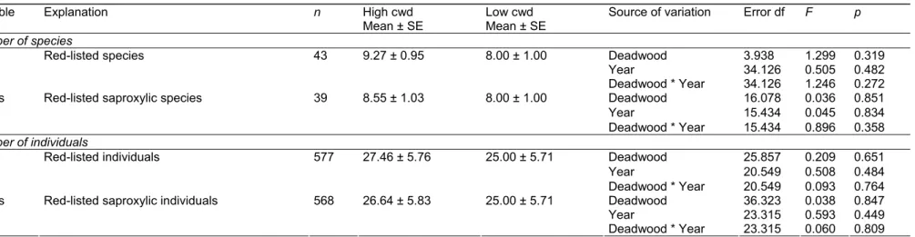
Also, neither the number of threatened species nor individuals varied significantly with the dead wood supply, despite most of the species (91%) being saproxylic (Table 6).

Another option to analyse the data in a way to disentangle dead wood from year effects was to carry on a GLM repeated measures ANOVA limited to those 11 stands rich in dead wood and use the extra information provided by trunk-window traps (a sampling device more efficient in catching rare and threatened saproxylic beetles than normal freely-hanging flight-window traps, Martikainen 2000). Among major findings, and as shown in our mixed models, we found that dead wood increased bark beetle abundance and more generally on the abundance of saproxylic beetles among which wood-living and mycetophageous beetles, although depending on the year (Appendices 12 & 13). From a species number point of view, only xylodetriticolous beetles showed a positive response, depending also on the year. But like in the mixed ANOVA procedure, we found that dead wood did not explain significant variation in the number of threatened insect species and individuals (Appendix 14).

Because of high between-year variation in insect captures, one way to improve the statistical power of our analyses was to sum up the number of species and individuals collected over the two sampling years (2002 + 2003). Using paired-sample t-tests to compare insect numbers between stand pairs, the number of saproxylic click beetles and of bark beetles was higher in stands classified as rich in

(34)

Table 5. Results of mixed-model ANOVA assessing differences in species richness (S) and abundance (A) of beetlesa between stands (11 pairs) with high

and low amount of coarse woody debris (cwd) (2002-2003). Saproxylic species are categorised either according to their micro-habitats or diet preferences following Köhler (2000).

Variable Explanation n High cwd

Mean ± SE

Low cwd Mean ± SE

Source of variation Error df F p Number of species

142 50.18 ± 2.53 47.64 ± 3.03 Deadwood 37.684 1.858 0.181

Year 19.450 0.241 0.629

S_be_s Saproxylic beetlesb

Deadwood * Year 19.450 0.010 0.923

41 12.36 ± 0.72 11.00 ± 0.63 Deadwood 85.820 0.443 0.508

Year 41.513 0.053 0.820

S_be_ns Non-saproxylic beetles

Deadwood * Year 41.513 1.317 0.258